Combinatorial Approach to Modeling Quantum Systems
Vladimir V. Kornyak1,a
1Laboratory of Information Technologies, Joint Institute for Nuclear Research,
141980 Dubna, Moscow Region, Russia
Abstract.Using the fact that any linear representation of a group can be embedded into permutations, we propose a constructive description of quantum behavior that provides, in particular, a natural explanation of the appearance of complex numbers and unitarity in the formalism of the quantum mechanics. In our approach, the quantum behavior can be explained by the fundamental impossibility to trace the identity of the indistinguishable objects in their evolution. Any observation only provides information about the invariant relations between such objects.
The trajectory of a quantum system is a sequence of unitary evolutions interspersed with observations — non-unitary projections. We suggest a scheme to construct combinatorial models of quantum evolution. The principle of selection of the most likely trajectories in such models via the large numbers approximation leads in the continuum limit to the principle of least action with the appropriate Lagrangians and deterministic evolution equations.
1 Introduction
Any continuous physical model is empirically equivalent to a certain finite model. This is widely used in practice: solutions of differential equations by the finite difference method or by using truncated series are typical examples. It is often believed that continuous models are “more fundamental” than discrete or finite models. However, there are many indications that the nature is fundamentally discrete at small (Planck) scales, and is possibly finite.1Moreover, the description of the physical systems by,
e.g., differential equations can not be fundamental in principle, since it is based on approximations of the form f(x)≈ f(x0)+∇f(x0)Δx. In this paper we consider some approaches to constructing
discrete combinatorial models of the quantum evolution.
The classical description of areversibledynamical system looks schematically as follows. There are a setW of states2 and a groupGcl ≤ Sym(W) of transformations (bijections) ofW. Evolutions
ofW are described by sequences of group elementsgt ∈Gclparameterized by the continuous time
t∈T=[ta,tb]⊆R. The observables are functionsh:W→R.
An arbitrary set W can be “quantized” by assigning numbers from a number systemF to the elementsw∈W, i.e., by interpretingWas a basis of the moduleF⊗W. The quantum description of a
ae-mail: [email protected]
1The total number of binary degrees of freedom in the Universe is about 10122as estimated via the holographic principle
and the Bekenstein–Hawking formula.
dynamical system assumes that the module spanned by the set of classical statesWis a Hilbert space HWover the field of complex numbers, i.e.,F =C. The transformationsgtand the observableshare
replaced by unitary,Ut∈Aut (HW), and Hermitian,H, operators onHW, respectively. A constructive
version of the quantum description is reduced to the following:
• time isdiscreteand can be represented as a sequence of integers, typicallyT=[0,1, . . . ,T]; • the setW is finite and, respectively, the spaceHWis finite-dimensional;
• the general unitary group Aut (HW) is replaced by a finite groupG;
• the fieldCis replaced byKth cyclotomic fieldQK, whereKdepends on the structure ofG; • the evolution operatorsUtbelong to a unitary representation ofGin the Hilbert spaceHWoverQK.
It is clear that a single unitary evolution isnot sufficientfor describing the physical reality. Such evolution is nothing more than a physically trivial change of coordinates (a symmetry transformation). This means that observable values or relations, being invariant functions of states, do not change with time. As an example, consider a unitary evolution of a pair of state vectors: |ϕ1 = U|ϕ0 ,
|ψ1 = U|ψ0 . For the scalar product we have ϕ1|ψ1 = ϕ0|U−1U|ψ0 ≡ ϕ0|ψ0 . There are
two ways to obtain observable effects in the scenario of unitary evolution: (a) in quantum mechanics measurements are described by non-unitary operators — projections into subspaces of the Hilbert space; (b) in gauge theories collections of evolutions are considered, and comparing results of different evolutions can lead to observable effects (in the case of a non-trivial gauge holonomy).
The role of observations in quantum mechanics is very important — it is sometimes said that “observation creates reality”.3We pay special attention to the explicit inclusion of observations in the
models of evolution. While the states of a system are fixed in the moments of observation, there is no objective way to trace the identity of the states between observations. In fact, all identifications — i.e., parallel transports provided by the gauge group which describes symmetries of the states — are possible. This leads to a kind of fundamental indeterminism. To handle this indeterminism we need a way to describe statistically collections of parallel transports. Then we can formulate the problem of finding trajectories with maximum probability that pass through a given sequence of states fixed by observations. In a properly formulated model, the principle of selection of the most probable trajectories should reproduce in the continuum limit the principle of the least action.
2 Constructive description of quantum behavior
The transition from a continuous quantum problem to its constructive counterpart can be done by replacing a unitary group of evolution operators with some finite group. To justify such a replace-ment [1] one can use the fact from the theory of quantum computing that any unitary group contains a dense finitely generated subgroup. Thisresidually finite[2] group has infinitely many finite homo-morphic images. The infinite set of non-trivial homomorphisms allows to find a finite group that is empirically equivalent to the original unitary group in any particular problem.
2.1 Permutations and natural quantum amplitudes
As it is well known, any representation of a finite group is a subrepresentation of some permuta-tion representapermuta-tion. Namely, a representapermuta-tion U ofGin a K-dimensional Hilbert spaceHKcan be embedded into a permutation representation P ofGin anN-dimensional Hilbert spaceHN, where
N≥K. The representation P is equivalent to an action ofGon a set of thingsΩ ={ω1, . . . , ωN}by permutations. IfK=Nthen UP. Otherwise, ifK<N, the embedding has the structure
T−1PT=
⎛ ⎜⎜⎜⎜⎜ ⎜⎜⎜⎝ 1 V
HN−K U} HK
⎞ ⎟⎟⎟⎟⎟
⎟⎟⎟⎠, HN=HN−K⊕ HK.
Here1is the trivial one-dimensional representation. It is a mandatory subrepresentation of any per-mutation representation. V is an optional subrepresentation. We can treat the unitary evolutions of data in the spacesHKandHN−Kindependently, since both spaces are invariant subspaces ofHN.
The embedding into permutations provides a simple explanation of the presence of complex num-bers and complex amplitudes in the formalism of the quantum mechanics. We interpret complex quantum amplitudes as projections onto invariant subspaces of vectors with natural components for a suitable permutation representation [1, 3, 4]. It is natural to assign natural numbers — multiplicities — to elements of the setΩon which the groupGacts by permutations. The vector of multiplicities,
|n =
⎛ ⎜⎜⎜⎜⎜ ⎜⎜⎜⎜⎜ ⎝
n1
.. .
nN
⎞ ⎟⎟⎟⎟⎟ ⎟⎟⎟⎟⎟ ⎠,
is an element of themoduleHN=NN, whereN={0,1,2, . . .}is thesemiringof natural numbers. The permutation action defines thepermutation representationofGin the moduleHN. Using the fact that all eigenvalues of any linear representation of a finite group areroots of unity, we can turn the module HNinto a Hilbert spaceHN. We denote byNK thesemiringformed by linear combinations ofKth
roots of unity with natural coefficients. The so-calledconductorKis a divisor of theexponent4ofG.
In the caseK >1 the semiringNK becomes aring of cyclotomic integers. The introduction of the cyclotomic fieldQK as the field of fractions of the ringNK completes the conversion of the module HNinto the Hilbert spaceHN. IfK >2, thenQK is empirically equivalent to the field of complex
numbersCin the sense thatQK is a dense subfield ofC.
2.2 Measurements and the Born rule
A quantum measurement is, in fact, a selection among all the possible state vectors that belong to a given subspace of a Hilbert space. This subspace is specified by the experimental setup. The probability to find a state vector in the subspace is described by the Born rule. There have been many attempts to derive the Born rule from other physical assumptions — the Schrödinger equation, Bohmian mechanics, many-worlds interpretation, etc. However, the Gleason theorem [5] shows that the Born rule is a logical consequence of the very definition of a Hilbert space and has nothing to do with the laws of evolution of the physical systems.
The Born rule expresses the probability to register a particle described by the amplitude |ψ by an apparatus configured to select the amplitude|φ by the formula (in the case of pure states):
P(φ, ψ)= |φ|ψ |
2
φ|φ ψ|ψ ≡
ψ|Πφ|ψ
ψ|ψ ≡tr ΠφΠψ
,
whereΠa=|
a a|
a|a is the projector onto the subspace spanned by |a .
Remark.In the “finite” background the only reasonable interpretation of probability is thefrequency
interpretation: probability is the ratio of the number of “favorable” combinations to the total number of combinations. So we expect thatP(φ, ψ) must be a rational number if everything is arranged correctly. Thus, in our approach the usualnon-constructivecontraposition — complex numbersas intermediate values vs. real numbersas observable values — is replaced by theconstructiveone —
irrationalitiesvs. rationals. From the constructive point of view, there is no fundamental difference between irrationalities and constructive complex numbers: both are elements of algebraic extensions.
2.3 Illustration: constructive view of the Mach–Zehnder interferometer
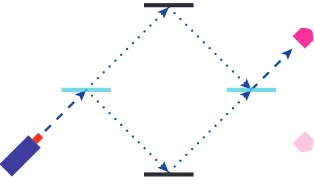
The Mach–Zehnder interferometer is a simple but important example of a two-level quantum system. The device consists of a single-photon light source, beam splitters, mirrors and photon detectors (see Figure 1). Consider a two-dimensional Hilbert space spanned by the two orthonormal basis vectors
Figure 1.Mach–Zehnder interferometer. Balanced setup: both beam splitters are 50/50 and there is no phase shift between upper and lower paths.
| — “right upward beams”, and | — “right downward beams”. Then the 50/50 beam splitter (i.e., a photon has equal probability of being reflected and transmitted) is described by the matrix
S = √1
2
1 i i 1
. (1)
The mirror matrix is M =
0 i i 0
. Notice thatM =S2, and, on the other hand,S can be expressed
viaMas an element of the group algebra:S = √1
2(I+M), where I is the identity matrix. The scheme
in the figure implements the unitary evolutionSMS| =S4| =− | , which means that only
the upper detector will register photons, the lower detector will always be inactive.
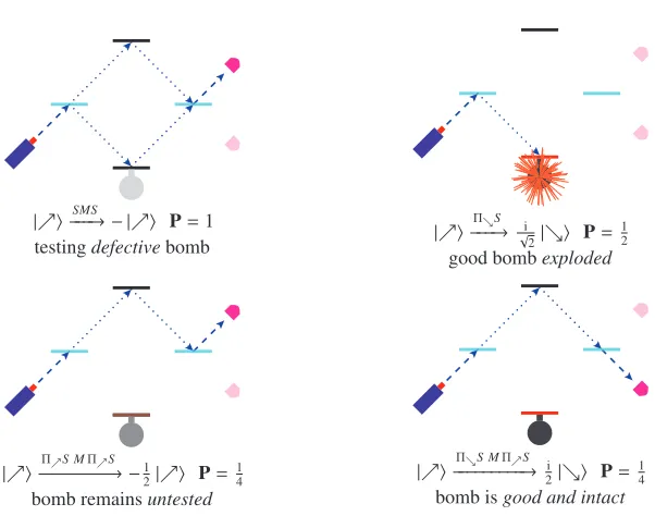
This device is able to demonstrate many interesting features of the quantum behavior. Consider, for example, the scheme of quantuminteraction-free measurement proposed by Elitzur and Vaid-man [6]. The Penrose’s version of this example is called thebomb-testing problem. Suppose we have a collection of bombs, of which some are defective. The detonator of a good bomb causes explosion after absorbing a single photon. The detonators of defective bombs reflect photons without any conse-quences. Classically, the only way to verify that a bomb is good is to touch the detonator. However, as shown in Figure 2, the quantum interference makes it possible to select 25% of good bombs without exploding them: the signal of the lower detector ensures that the unexploded bomb is good.
A slight modification of the scheme shown in Figure 1 allows us to implement any unitary opera-torU∈U(2) by the Mach–Zehnder interferometer. This is easily verified by direct calculation. Since dimU(2)=4, we should add four parameters in a proper way. For example, we can change the trans-parency of the beam splitter. Mathematically this means replacing the matrix (1) by another one of the formαI+βM, where |α|2+|β|2=1. Another possibility is to introducephase shifters. The phase
shifter matrix related, e.g., to a “right upward beam” has the form
eiω 0
0 1
. Moreover, combining
| −−−→ − | SMS P=1
testingdefectivebomb |
ΠS
−−−→ √i
2| P= 1 2 good bombexploded
| −−−−−−−−−→ −ΠS MΠS 1
2| P= 1 4 bomb remainsuntested
| −−−−−−−−−→ΠS MΠS i
2| P= 1 4 bomb isgood and intact
Figure 2.Penrose bomb tester.Pis the probability of a branch of evolution.Πadenotes the projector onto |a.
Since a “mirror” is the square of a “beam splitter”, any unitary evolution in a sequence of balanced Mach–Zehnder interferometers can be described by degrees ofS. The operatorS generates the cyclic groupZ8. The smallest degree faithful action ofZ8is realized by permutations of 8 objects. Any of
the four permutations, that generateZ8as a group of permutations, can be put in correspondence with
the beam splitter, e.g.,S ←→g=(1,2,3,4,5,6,7,8). The generatorgcan be represented by a matrix
Pgacting in the moduleN8that consists of the vectors with natural components:
N=(n1,n2,n3,n4,n5,n6,n7,n8)T ∈N8.
To “extract” the beam splitter from the matrixPgwe should extend the natural numbers by 8th roots of unity — the conductorK =8 in this case. Any 8th root of unity can be represented as a power of any of the fourprimitiveroots defined by thecyclotomic polynomialΦ8(r)=r4+1. Let us denote by
N8 the set of linear combinations of 8th roots of unity with natural coefficients. This is a ring since
K=8>1. The ringN8is isomorphic to the ring of 8th cyclotomic integers. In principle, due to the
projective nature of the quantum states, we could perform all calculations using only natural numbers and roots of unity. But it is convenient to use also the 8th cyclotomic field, which we will denote by Q8. The fieldQ8is the fraction field of the ringN8.
The matrixPgby a transformationT over the fieldQ8can be reduced to the form
Sg=T−1PgT =
A 0 0 Sr
,
whereA=diag 1,−1,r2,−r2,r3,−r, r is a primitive 8th root of unity, and
Sr=
1 2
r−r3 r+r3
r+r3 r−r3
is the beam splitter matrixS expressed in terms of cyclotomic numbers. The quantum amplitude of the Mach–Zehnder interferometer can be approximated by the projection of the natural vectorNinto the “splitter” subspace:
|ψ =
ψ1
ψ2
= 1 8
⎛ ⎜⎜⎜⎜⎜ ⎝−r
3(n
1+n3−n5−n7)+ 1−r2
(n2−n6)
r (n1−n3−n5+n7)+ 1+r2
(−n4+n8) ⎞ ⎟⎟⎟⎟⎟
⎠. (3)
It can be shown that the expression (3) can approximate with arbitrary precision any point on the Bloch sphere — a standard representation of the complex projective lineCP1.
3 Combinatorial models of evolution
Let us begin with some general considerations concerning the evolution of the probabilistic systems subject to observations. The evolution of such a system can be described as follows. We have a fundamental (“Planck”) time which is the sequence of integers:
T=[0,1, . . . ,T]. (4) There is also a sequence of “times of observations”. For simplicity, we assume that the observation time is a subsequence of the fundamental time
T =[t0=0, . . . ,ti−1,ti, . . . ,tN =T] (5)
(otherwise we could assume that the times of the observations are not determined exactly, e.g., they could be random variables with probability distributions localized within subintervals of the funda-mental time). LetWtidenote the state of a system observed at the timeti, and
Wt0→ · · · →Wti−1→Wti → · · · →WtN (6)
denote a trajectory of the system. Whereas the statesWti−1 and Wti are fixed by observation, the transition between them can be described only probabilistically.
The selection of the most probable trajectories is the main problem in the study of the evolution. If we can specifyPWti−1→Wti— theone-step transition probability— then the probability of trajectory (6) can be calculated as the product
PWt0→···→WtN =
N
i=1
PWti−1→Wti. (7)
The inconvenience of dealing with the product of large number of multipliers can be eliminated by introducing theentropy, which is defined as the logarithm of probability. The transition to logarithms allows us to replace the products by sums. On the other hand, taking the logarithm does not change the positions of the extrema of a function due to the monotonicity of the logarithm. Thus, for searching the most likely trajectories we introduce theone-step entropy
SWti−1→Wti =logPWti−1→Wti (8)
and use instead of (7) theentropy of trajectory:
SWt0→···→WtN =
N
i=1
The formulation of any dynamical model usually begins with postulating a Lagrangian. However, it would be desirable to derive Lagrangians from more fundamental principles. One can see that con-tinuum approximations of (8) and (9) lead to the concepts of Lagrangian and action, respectively. The reasoning is schematically the following. The statesWtiare specified by sets of numerical parameters (coordinates)Xti =
X1,ti,X2,ti, . . . ,XK,ti
. For a specific model one-step entropy (8) can be calculated as a function of the coordinates: SWti−1→Wti =SXti,ΔXti
, whereΔXti =Xti−Xti−1. Assuming that
N→ ∞,ti−ti−1 →0 and embedding the sequenceXtiinto the continuous functionX(t), we can rep-resent the one-step entropy in the formS(X(ti),ΔX(ti)).The second order Taylor approximation of
this function has the formS ≈A+bkk ΔXk(ti)−ΔX∗k(ti)
ΔXk(ti)−ΔX∗k(ti)
, whereΔX∗(ti) is the
solution of the system of equations ∂S
∂ΔX(ti)
=0.Since the discrete time is a dimensionless counter, the differences can be approximated in the continuum limit by introducing derivatives, and we come to the Lagrangian
L=A+Bkk
dXk
dt −ak dXk
dt −ak
,
whereBkkis anegative definitequadratic form; Bkk, Aandakdepend onX1(t),X2(t), . . . ,XK(t).
The action
S=
Ldt
is a continuum approximation of the entropy of trajectory (9), so the principle of least action can be treated as a continuous remnant of the principle of selection of the most likely trajectories.
3.1 Example: extracting Lagrangian from combinatorics
As an illustration of the above let us consider the one-dimensional random walk. This model studies the statistics of sequences of positive (+1) and negative (−1) unit steps on the integer lineZ. Any statistical description is based on the concepts ofmicrostates andmacrostates— the last can naturally be treated as equivalence classes of microstates [8]. In this model, microstates are individual sequences of steps. The probability of a microstate consisting ofk+positive andk−negative steps is equal toαk+
+αk−−, whereα+andα−denote probabilities of single steps (α++α−=1). The macrostates are defined by the equivalence relation: two sequencesuandvare equivalent ifku
++ku−=kv++kv−=t
andku
+−k−u =kv+−kv− = x, i.e., both sequences have the same lengthtand define the same pointx
onZ. The probability of an arbitrary microstate to belong to a given macrostate is described by the binomial distribution, which in terms of the variablesxandttakes the form
P(x,t)= t!
t+x 2
! t−2x!
1+v 2
t+x
2 1−v
2
t−x
2
, (10)
wherev=α+−α−is the “drift velocity”.5 Obviously, −1≤v≤1.
Let [x0, . . . ,xi−1,xi, . . . ,xN] be a sequence of points (observed values) corresponding to the
se-quence of times of observations (5). We assume that the time differencesΔti = ti−ti−1 are much
larger than the unit of fundamental time (4) but much less than the total time: 1ΔtiT. Applying
formula (10) toith time interval we can write the one-step entropy:
Sxi−1→xi =lnΔti!−ln
Δti+ Δxi
2
!−ln
Δti−Δxi
2
!+Δti+ Δxi 2 ln
1+vi
2
+Δti−Δxi
2 ln
1−vi
2
,
whereΔxi=xi−xi−1, andvidenotes the drift velocity in theith interval.
Applying the Stirling approximation, lnn!≈nlnn−n, we have
Sxi−1→xi≈Si= ΔtilnΔti−
Δti+ Δxi
2 ln
Δti+ Δxi
1+vi
−Δti−Δxi
2 ln
Δti−Δxi
1−vi
. (11)
Solving the equation∂Si/∂Δxi = 0 we obtain the stationary point: Δx∗i = viΔti. Replacing the
sequencesxi, viby continuous functionsx(t), v(t) and introducing the approximationΔxi ≈x˙(t)Δti
in the second order Taylor expansion of (11) around the pointΔx∗i we have finally
Sxi−1→xi≈ − 1 2
˙ x(t)−v √
1−v2 2
Δti.
Thus we come to the LagrangianL=
˙ x(t)−v √
1−v2 2
with the corresponding Euler-Lagrange equation
d dt
∂L
∂x˙ −
∂L
∂x =0 =⇒ x¨ 1−v
2+2 ˙xv∂v
∂t − 1+v
2∂v
∂t =0.
3.2 Scheme for constructing models of quantum evolution
The trajectory of a quantum system is a sequence of observations with unitary evolutions between them. We propose a scheme to construct quantum models that combine unitary evolutions with ob-servations. The scheme assumes that transitions between observations are described by bunches of properly weighted unitary parallel transports. The standard scheme of quantum mechanics with single unitary evolutions can be reproduced in our scheme by a special choice of weights. But in our scheme such unique evolutions are assumed to be obtained as statistically dominant elements of the bunches.
We use the following notations • H: a Hilbert space;
• Πψt0, . . . ,Πψti, . . . ,ΠψtN: a sequence of observations, whereΠψti =ψti
ψ
tiis the projector that fixesψti ∈ Has the result of observation at the timeti; • Δti=ti−ti−1: the length ofith time interval;
• G={g1, . . . ,gM}: a finitegauge group;
• U: a unitary representation ofGin the spaceH;
• γ=g1, . . . , gΔti: a sequence of the lengthΔtiof elements fromG; • val(γ)=Δti
j=1gj∈G: the (group)valueof the sequenceγ— the parallel transport;
• Γi=γ1, . . . , γk, . . . , γKi
: an (arbitrary)enumerationof the set of all sequencesγ, whereKi≡ |Γi|=MΔti is the total number of the sequences;
• wki: anon-negative weightofkth sequence (inith time interval).
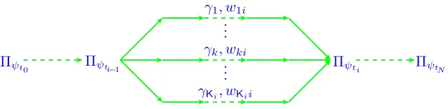
With these notations we come to the scheme shown in Figure 3. The probability of transition from
ψti−1toψtiis given by the formula
Pψti−1→ψti = Ki
k=1
Πψt0 Πψti−1
γ1, w1i ...
γk, wki ...
γKi, wKii
Πψti ΠψtN
Figure 3.Scheme of quantum evolution with observations
The case of standard quantum mechanics with a single unitary evolution between observations is obtained in our scheme by selecting a sequenceγformed by an elementg ∈ GrepeatedΔtitimes.
The weight of the sequenceγis set to 1, and the weights of all other sequences are equated to 0. In other words, the set of weights is the Kronecker delta on the set of sequences: wki =δγ,γk, γk ∈ Γi.
Introducing the HamiltonianH=i ln U(g), we can write the evolution in the usual form
U≡U gΔti=e−iH(ti−ti−1).
Since the notion of Hamiltonian stems from the principle of least action, it is natural to assume the existence of some mechanism of selecting sequences of the formg, g, . . . , gas dominant elements in the set of all sequences. This requires a detailed analysis of the combinatorics of steps in fundamental time (4) for particular models.
3.3 Dynamics of observed quantum system. Quantum Zeno effect and finite groups
Consider the issue concerning the connection between the quantum dynamics and the group properties of unitary evolution operators. Namely, we consider the quantum Zeno effect for operators that belong to representations of finite groups.
The “quantum Zeno effect”6(see the review [10]) is a feature of the quantum dynamics, which is
manifested in the fact that frequent measurements can stop (or slow down) the evolution of a system — for example, inhibit decay of an unstable particle — or force it to evolve in a prescribed way. In the latter case, the phenomenon is called the “anti-Zeno effect”.
Consider a quantum system that evolves from the initial (att = 0) normalized pure state |ψ0
under the action of the unitary operatorU =e−iHt, whereHis the Hamiltonian. The probability to
find the system in the initial state at the timetis the following
pH(t)=
ψ0e−iHtψ0 2
. (12)
The most important characteristics of any dynamical process are its temporal parameters. For the quantum Zeno effect such a parameter is called the “Zeno time”, denotedτZ. It is determined from
the short-time expansion of (12):
pH(t)=1−t2/τ2Z+O t4
. (13)
Calculation of (13) shows that τ−Z2=ψ0H2ψ0
−ψ0Hψ0 2
.
Let us present the so-calledZeno dynamicsin the framework of scheme proposed in Section 3.2. We have here the sequence of observationsΠψt
0,Πψt1, . . . ,ΠψtN, each of which selects the same state
ψ0, i.e.,ψt0 =ψt1 =· · ·=ψtN ≡ψ0. Assuming thatt0=0, tN =T and the times of observations are equidistant:ti−ti−1 =T/N, we can write, using (13), the approximation for the one-step transition
probability
Pψti−1→ψti ≈1− 1 N2
T
τZ 2
with the corresponding approximation for the one-step entropy
Sψti−1→ψti ≈ − 1 N2
T
τZ 2
.
For the entropy of the trajectory we have
Sψt0→···→ψtN =
N
i=1
Sψti−1→ψti ≈ −1 N
T
τZ 2
N→ ∞
−−−−−→0
and, respectively, for the probability of trajectory: Pψt
0→···→ψtN
N→ ∞
−−−−−→e0=1. This is precisely the essence of the Zeno effect.
Now assume that the evolution operatorUbelongs to a representation of a finite groupG, i.e., U = U (g), g ∈ G, and the time is the sequence of natural numbers: t = 0,1,2, . . . . A natural way to define the Zeno time in this case follows from the observation that the leading part of the expansion (13) vanishes att =τZ. By analogy we can define thenatural Zeno time
τ
Z as the firstt∈[0,1,2, . . .] that provides minimum of the expression
pU(t)=
ψ0Utψ0 2
. (14)
Obviously, the expression (14) is either constant (namely, pU(t) =1) or periodic. In the latter case
its period is a divisor of the order ofU. Theorderof an elementaof a group is the smallest natural numbern>0 such thatan=e, whereedenotes the identity element of the group. The order ofawill be denoted ord (a). For the faithful representation, ord (U)≡ord (U (g))=ord (g).
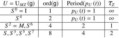
Consider, for example, the “Max-Zehnder” representation UMZ of the groupZ8, i.e., the “beam
splitter” matrix (1) is taken as a generator ofZ8. Table 1 presents the Zeno times for all operators
from the representation UMZ. We adopt the convention (motivated by formula (13)) that
τ
Z =∞if theprobability (14) is constant.
Table 1.Zeno times for all operators from UMZ(Z8)
U=UMZ(g) ord(g) Period(pU(t))
τ
ZS0=I 1 p
U(t)=1 ∞
S4 2 p
U(t)=1 ∞
S2=M,S6 4 2 1
S,S3,S5,S7 8 4 2
The two-dimensional “Max-Zehnder” representation UMZ can be generalized to the arbitrary
cyclic groupZNby replacing the “beam splitter” matrix of the form (2) with the unitary matrix
SN =
1 2
r+rN−1 r−rN−1
r−rN−1 r+rN−1
where r is anNth primitive root of unity. Figure 4 shows the evolution of the probability to observe the initial state for the evolution operatorS100in the time interval 0≤t≤100. The quadratic
short-time behavior, described by the formula (13), is clearly visible in the figure. The Zeno short-time in this example is
τ
Z=25.Figure 4.ProbabilitypU(t) vs. timetfor the operatorU=S100∈UMZ(Z100).
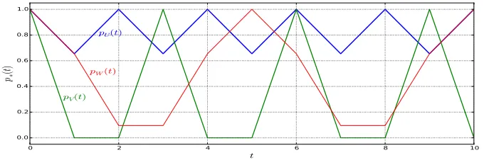
As a non-commutative example, consider the icosahedral groupA5 — the smallest (|A5| =60)
non-commutative simple group. It has applications for model building in the particle physics, espe-cially in issues beyond the standard model, such as the flavor physics [11]. The non-trivial elements of A5have orders 2, 3 and 5. The irreducible representations ofA5are: one trivial singlet,1, two triplets,
3and3, one quartet,4, and one quintet,5. Figure 5 shows the evolution of the “Zeno probabilities” for the following matrices of orders 2, 3 and 5, respectively,
U= 1 2
⎛ ⎜⎜⎜⎜⎜
⎜⎜⎜⎝1−/φφ 1−/φ1 1φ 1 φ 1/φ
⎞ ⎟⎟⎟⎟⎟ ⎟⎟⎟⎠,V =
⎛ ⎜⎜⎜⎜⎜
⎜⎜⎜⎝01 00 10 0 1 0
⎞ ⎟⎟⎟⎟⎟
⎟⎟⎟⎠, W =1 2
⎛ ⎜⎜⎜⎜⎜
⎜⎜⎜⎝1−/φφ −11/φ 1φ −1 φ −1/φ
⎞ ⎟⎟⎟⎟⎟
⎟⎟⎟⎠, (15)
whereφ = 1+2√5 is the “golden ratio”. To write these matrices, we added an element of order 3 (the simplest among randomly selected) to the generators of orders 2 and 5 proposed in [12] for the representation3.
4 Summary
1. We adhere to the idea of empirical universality of discrete, more specifically, finite models for describing physical reality. In other words, any continuous model can be replaced by a finite model that fit the same observable behavior.
2. This idea, in application to quantum problems, means that unitary groups of evolution operators can be replaced by unitary representations of finite groups.
3. The mathematical fact that any representation of a finite group can be embedded in a permuta-tion representapermuta-tion allows to approximate, with arbitrary precision, the quantum amplitudes by projections of vectors with natural components. The complex components of these projections are combinations of natural numbers and roots of unity.
4. To illustrate the content of the article, we have used the Mach-Zehnder interferometer — a simple but important example of a two-level quantum system with rich behavior.
5. We propose a scheme for constructing quantum models. Taking into account that a single unitary evolution, being a simple change of coordinates, is not sufficient to describe the physical phenomena, the scheme involves sequences of observations with bunches of unitary parallel transports between the observations.
6. The principle of selection of the most probable trajectories in such models via the large numbers approximation leads in the continuum limit to the principle of the least action with appropriate Lagrangians and deterministic evolution equations.
7. To look at the connection between quantum dynamics and the group properties of unitary evo-lution operators, we have considered the quantum Zeno effect in the context of our approach.
Acknowledgements
The work is supported in part by the Ministry of Education and Science of the Russian Federation (grant 3003.2014.2) and the Russian Foundation for Basic Research (grant 13-01-00668).
References
[1] Kornyak V.V., Phys. Part. Nucl.44, 47–91 (2013); http://arxiv.org/abs/1208.5734 [2] Magnus W., Bull. Amer. Math. Soc.75, No 2, 305–316 (1969)
[3] Kornyak V.V., J. Phys.: Conf. Ser.343(2012) 012059
http://iopscience.iop.org/1742-6596/343/1/012059 [4] Kornyak V.V., J. Phys.: Conf. Ser.442(2013) 012050
http://iopscience.iop.org/1742-6596/442/1/012050 [5] Gleason A.M., Indiana Univ. Math. J.6, 885–893 (1957)
[6] Elitzur A. and Vaidman L., Foundation of Physics23, 987–997 (1993)
[7] Reck M., Zeilinger A., Bernstein H.J., Bertani P., Phys. Rev. Lett.73, 58–61 (1994) [8] Kornyak V.V., Math. Model. Geom.3, 1–24 (2015); http://arxiv.org/abs/1501.07356 [9] Knuth K.H., AIP Conf. Proc.1641, 588 (2015); http://arxiv.org/abs/1411.1854 [10] Facchi P., Pascazio S., J. Phys. A: Math. Theor.41(2008) 493001
doi:10.1088/1751-8113/41/49/493001