Evaluation of precise point positioning services

University of Southern Queensland

Faculty of Engineering and Surveying

Evaluation of Precise Point Positioning Services

A dissertation submitted by

Mr. Daniel O’Sullivan

In fulfilment of the requirements of

Course ENG4111 and ENG4112 – Research Project

Towards the degree of

Bachelor of Spatial Science (Surveying)

ABSTRACT

Precise Point Positioning (PPP) is a Global Navigation Satellite System (GNSS) positioning method which enables the calculation of a precise position utilising a single geodetic quality GNSS receiver and PPP software. There has been a range of research which has examined the accuracy and reliability of freely available online PPP services. This study will look to confirm the results of previous findings and follow up on some gaps identified in existing research.

This study compared the performance of AUSPOS, OPUS, CSRS-PPP and Magic PPP. It initially compared them to existing Survey Control Information Management System (SCIMS) coordinated survey marks but discovered the SCIMS coordinates were not suitable for comparison. It examined solutions for bias as well as comparing the differential baseline processing method to true PPP method. It examined the effect of including GLONASS satellite observation data with GPS satellite observation data in order to develop a solution and it compared the results to previous studies in order to test the reliability of research to date.

LIMITATIONS OF USE

The Council of the University of Southern Queensland, its Faculty of Health, Engineering & Sciences, and the staff of the University of Southern Queensland, do not accept any responsibility for the truth, accuracy or completeness of material contained within or associated with this dissertation.

Persons using all or any part of this material do so at their own risk, and not at the risk of the Council of the University of Southern Queensland, its Faculty of Health, Engineering & Sciences or the staff of the University of Southern Queensland.

This dissertation reports an educational exercise and has no purpose or validity beyond this exercise. The sole purpose of the course pair entitled “Research Project” is to contribute to the overall education within the student’s chosen degree program. This document, the associated hardware, software, drawings, and other material set out in the associated appendices should not be used for any other purpose: If they are so used, it is entirely at the risk of the user.

CANDIDATES CERTIFICATION

I certify that the ideas, designs and experimental work, results, analysis and conclusions set out in this dissertation are entirely my own efforts, except where otherwise indicated and acknowledged.

I further certify that the work is original and has not been previously submitted for assessment in any other course or institution, except where specifically stated.

Daniel Francis O’Sullivan Student Number: W0100225

(Signature)

ACKNOWLEDGEMENTS

This research was carried out under the principal supervision of Associate Professor Peter Gibbings. I would like to thank Professor Gibbings for his tips, guidance and support throughout.

LIST OF FIGURES

Number

Title

Page

3.1 Aerial Photo of Hayter Trig Station, Coopers Shoot 17 3.2 Site Photo of Hayter Trig Station, Meerschaum Vale 17

3.3 Aerial Photo of Meershaum Trig Station 18

3.4 Site Photo of Meerschaum Trig Station 18

3.5 Aerial Photo of North East NSW 19

3.6 IGS Tracking Network 20

3.7 APREF Network of CORS in the Australian Region

(Geoscience Australia, 2014) 20

4.1 Plot of Comparison of SCIMS Coordinates, SCIMS

Coordinates Transformed to ITRF2008 and the Average of the

Processed Solutions (Origin) at Hayter Trig Station 27

4.2 Plot of 24hr Solutions - Hayter Trig 29

4.3 Plot of Comparison of SCIMS Coordinates, SCIMS

Coordinates Transformed to ITRF2008 and the Average of the

Processed Solutions (Origin) at Meerschaum Trig Station 30

4.4 Plot of 24hr Solutions - Meerschaum Trig 31

4.5 Plot of GPS vs GNSS Solutions – Hayter Trig 37

4.6 Plot of GPS vs GNSS Solutions – Meerschaum Trig 38

5.1 95% Confidence Interval of Residuals- Differential Baseline Solutions 41 5.2 95% Confidence Interval of Residuals – PPP Solutions 41 5.3 Combined 95% Confidence Interval of Residuals – Differential

Baseline vs PPP 42

5.4 95% Confidence Interval of Residuals - CSRS GPS vs CSRS GNSS 43 5.5 95% Confidence Interval of Residuals – Magic GPS vs Magic GNSS 44 5.6 95% Confidence Intervals of Residuals – Combined GPS vs

Combined GNSS 45

5.7 Comparison of Coordinate Residuals to Observation Time

– Differential Baseline Solutions 46

5.8 Comparison of Coordinate Residuals to Observation Time

LIST OF TABLES

Number

Title

Page

Table 2.1 Publicly Available Online Post Processing Services 10 Table 4.1 AUSPOS 24hr Observation Solutions – Hayter Trig 28 Table 4.2 OPUS 24hr Observation Solutions - Hayter Trig 28 Table 4.3 CSRS 24hr Observation Solutions – Hayter Trig 28 Table 4.4 Magic 24hr Observation Solutions – Hayter Trig 28 Table 4.5 AUSPOS 24hr Observation Solutions – Meerschaum Trig 31 Table 4.6 OPUS 24hr Observation Solutions – Meerschaum Trig 31 Table 4.7 CSRS 24hr Observation Solutions – Meerschaum Trig 31 Table 4.8 Magic 24hr Observation Solutions – Meerschaum Trig 31 Table 4.9 Residuals by Observation Length – Hayter Trig Station 33 Table 4.10 Residuals by Observation Length – Meerschaum Trig Station 34 Table 4.11 Comparison of 24hr GPS and GNSS Solutions – Hayter Trig Station 36 Table 4.12 Comparison of 24hr GPS and GNSS Solutions Meerschaum Trig

Station 36

Table 5.1 Solution Residuals 42

Table 5.2 GPS Average Solutions–3hr Residuals 43

LIST OF APPENDICES

Number Title

Page

A Project Specification 54

B Solutions by Observation Length 56

C 3hr Residuals 58

D RINEX File Example 61

E Leica Viva GNSS GS14 Specification 62

F SCIMS Survey Mark Reports 66

NOMENCLATURE AND ACRONYMS

The following abbreviations have been used throughout the text and bibliography:-

AHD Australian Height Datum AHD71 Australian Height Datum 1971 APREF Asia Pacific Reference Frame

CORS Continually Operating Reference Station ECEF Earth Centred Earth Fixed

ESTR89 European Terrestrial Reference Frame 1989 FCN Frequency Channel Number

GDA94 Geocentric Datum of Australia 1994

GLONASS Globalnaya navigatsionnaya sputnikovaya sistema (Global Navigation Satellite System)

GNSS Global Navigation Satellite System GPS Global Positioning System

ICSM Intergovernmental Committee on Surveying and Mapping IGS International GNSS Service

IGS08 International GNSS Service 2008

ITRF International Terrestrial Reference Frame ITRF2008 International Reference Frame 2008 LPI Land and Property Information NAD83 North American Datum 1983 PPP Precise Point Positioning

RINEX Receiver Independent Exchange Format RTK Real Time Kinematic Surveying

SCIMS Survey Control Information Management System

TABLE OF CONTENTS

CONTENTS

Page

ABSTRACT ... ii

LIMITATIONS OF USE ... iii

CANDIDATES CERTIFICATION ... iv

ACKNOWLEDGEMENTS ... v

LIST OF FIGURES ... vi

LIST OF TABLES ... vii

LIST OF APPENDICES ... viii

NOMENCLATURE AND ACRONYMS ... ix

CHAPTER 1 - INTRODUCTION ... 1

1.1 Background Information ... 1

1.2 Research Aim and Objectives ... 3

1.3 Justification ... 4

1.4 Summary ... 5

CHAPTER 2 - LITERATURE REVIEW... 6

2.1 Introduction. ... 6

2.2 Geodetic Surveying ... 6

2.3 Equipment ... 7

2.3.1 GNSS Receivers ... 7

2.4 On Line Post-Processing ... 7

2.4.1 Precise Point Positioning ... 8

2.4.2 Differential Baselines – Differential GNSS (DGNSS). ... 8

2.4.3 Online Post Processing Services ... 9

2.6 Previous Research ... 11

2.6.1 Cleaver ... 11

2.6.2 Silver ... 11

2.6.3 Tsakiri ... 12

2.6 Summary ... 13

CHAPTER 3 - METHOD ... 13

3.1 Introduction ... 13

3.2 Project Constraints ... 14

3.2.1 Equipment ... 15

3.2.2 Field Method ... 15

3.2.3 Survey Sites ... 16

3.3 Data Processing ... 19

3.3.1 Raw data ... 19

3.3.2 Processed data ... 19

3.3.3 AUSPOS ... 20

3.3.4 OPUS ... 21

3.3.5 Magic GNSS ... 21

3.3.6 Canadian Spatial Reference System PPP (CSRS-PPP) ... 22

3.5 Data Comparisons ... 22

3.5 Summary ... 23

CHAPTER 4 – RESULTS ... 24

4.1 Introduction ... 24

4.2 Processed Solutions ... 24

4.2 Twenty-Four-Hour Observation Solutions ... 26

4.2.1 Hayter Trig Station 24hr Observation Solutions ... 27

4.2.2 Meerschaum Trig Station 24hr Observation Solutions ... 30

4.3 Solutions by Observation Length ... 32

4.3.1 Residuals by observation length ... 33

4.4 Solution by Data Type ... 35

4.5 Summary ... 38

CHAPTER 5 – DATA ANALYSIS ... 39

5.1 Introduction ... 39

5.2 Three-Hour Solution Comparison ... 39

5.2.1 Residuals ... 40

5.2.2 Repeatability ... 41

5.3 Differential Baseline vs PPP ... 42

5.4 GPS vs GNSS ... 43

5.5 Solution Bias ... 46

5.6 Summary ... 48

CHAPTER 6 – CONCLUSION ... 49

6.1 Introduction ... 49

6.2 Recommendations ... 49

6.3 Conclusion ... 49

CHAPTER 7 - REFERENCES ... 51

APPENDICES ... 54

Appendix A Project Specification ... 54

Appendix B Solutions by Observation Length ... 56

Appendix C 3hr Residuals ... 58

Appendix D RINEX File Example ... 61

Appendix E Leica Viva GNSS GS14 Specification ... 62

Appendix F SCIMS Survey Mark Reports ... 66

CHAPTER 1 - INTRODUCTION

1.1 Background Information

The use of Global Navigation Satellite Systems (GNSS) products and services is now common place in human life. It is seen in navigation, machine guidance, surveying, network development, mapping and even in sports. Advances in technology have made GNSS products and services more affordable, more accessible and more accurate, increasing their use within society generally.

The surveying profession has embraced the technology, recognising the efficiencies it provides. Real Time Kinematic (RTK) surveying has been the preferred method used in cadastral and construction surveying. It comprises two GNSS satellite receivers, one a base station placed in a fixed position, the second a roving unit which is transported from place to place recording observations in the area being surveyed in real time. RTK relies upon the ability of the system to provide real time corrections to solutions at the roving unit.

In applications where a real time position is not a requirement, the single receiver static data is post processed in order to compute a solution. Whilst this means a delay or added step in the process of developing control, the use of a single receiver still offers a viable, cost effective alternative when establishing a coordinated network in places where few if any coordinated networks exist.

Precise Point Positioning (PPP) is essential in single receiver observations in order to correct for the various errors that are inherent in raw observation data. These errors are caused by such things as atmospheric composition, differences in satellite and receiver clock accuracies, differences in modelled and actual satellite position and orientation and geological effects. Fortunately post processing has been aided by the provision of freely available online processing services. These online services utilise either a traditional differential baseline processing method or true PPP to develop a solution (Tsikiri, 2008).

Differential baseline processing utilises the nearest continually operating reference stations (CORS) with known coordinates and forms baselines between those and the occupied mark. It does this by processing raw data from the receiver and generates the baselines formed by the network of stations and the point being surveyed to calculate corrected solutions. PPP post processing utilises a different method of processing the data. It uses the undifferenced carrier phase and code phase observations and requires accurate knowledge of satellite coordinates as well as the state of their clocks and earth rotation parameters in order to process a solution (Martin et al, 2010). Whilst both methods have differences at the modelling level and with data control algorithms, both employ the same fundamental mathematical principals (Tsakiri, 2008, pp 116).

may be possible to provide guidance on what service might be suitable for a given scenario.

More studies are required in order to confirm the reliability and accuracy of the results obtained by the various methods of PPP. In addition there needs to be more focus on whether a bias impacts the final solution and to what extent. This study aims to confirm the results of previous research as well as to address the identified gaps. Solutions generated from identical data will be compared for bias between processing methods and raw Global Positioning System (GPS) observations will be compared with solutions where GPS and GLONASS observations are combined.

1.2 Research Aim and Objectives

The aim of the project is to evaluate and compare the performance of PPP and

differential baseline methods of online post processing services, when processing the

same data captured over extended periods of time and in multiple data collection

sessions. This will be achieved by statistically analysing the accuracy and precision of

processed solutions, comparing solutions from each method of post processing to

identify the existence of any bias and comparing the processed solutions to the known

coordinates.

The objectives of the study are to:

1. Establish background knowledge of relevant geodetic surveying practices, data collection methods, equipment and GNSS post processing services,

2. Research the differences between true PPP and differential GNSS post processing services,

3. Identify service providers and research methods of online post processing (eg Trimble’s RTX, CSRS from Natural Resources Canada, Auspos from Geoscience Australia and OPUS, the United States Government run service from the National Geodetic Survey website.

4. Research Statistical Analysis,

5. Develop a method for data collection that will allow the necessary comparisons to be made,

7. Evaluate results of data analysis to determine if any bias exists between the different methods of post processing,

8. Compare post-processed solutions to known coordinates to evaluate accuracy and precision of solutions for different logging times,

9. Compare solutions from GPS derived post processed data to that of solutions derived from GPS and GLONASS data in order to evaluate accuracy and precision, and

10. Examine repeatability of results by comparing solutions from data collected over multiple sessions and multiple days.

1.3 Justification

Previous studies have identified the role GNSS can play in geodetic surveying and in particular the development of survey control in areas where little if anything in the way of an established coordinated network exists. One of the significant challenges in this scenario is developing a coordinated network in a cost effective and efficient manner. Utilising static observation data and post processing services enables the development of a collection of control points with suitably accurate coordinates in an efficient and cost effective way.

These post processing services will quickly and easily produce output. However, users must be confident that the data they are producing is suitably accurate and precise for the intended use. A greater understanding of how these services produce a solution will enable more confidence to be placed in the output and will help users decide which service might be suitable for their particular application.

order to compare results and examine reliability and repeatability. In addition to this, the introduction of GLONASS satellite data and other GNSS constellations into post processing services requires research in order to ascertain what if any effect these have on a final processed solution.

Therefore, there is a need to process data collected over multiple days and sessions from multiple sites in order to better examine reliability and repeatability of the method and thus augment the results of previous studies. Observations taken at all sites at the same time will enable the isolation of the effects of some errors. There is also a need to compare processing methods for the existence of any bias, as this has been identified but not extensively examined in research to date. This will enable the effects of bias to be considered in the context of the project being undertaken and a decision made on the suitability of one service or processing method over another.

1.4 Summary

CHAPTER 2 - LITERATURE REVIEW

2.1 Introduction.

To progress this research it is necessary to examine background information on geodetic surveying and the equipment and systems used in determining accurate and precise three dimensional point coordinates. An examination of research to date in the field of post processing details the gaps in this research which have been identified in Chapter 1.

The aim of this chapter is to gain sufficient understanding of geodetic surveying and post processing techniques. This will enable the planning and preparation of a suitable project method to examine precise point positioning and critically and statistically analyse results in order to draw appropriate conclusions and recommendations.

This will be done by identifying suitable equipment and survey sites as well as researching freely available, online post processing services that would be suitable for post processing raw GNSS observation data. It will also examine the research to date, identifying what gaps, limitations or shortfalls exist and how these will be addressed in this study.

2.2 Geodetic Surveying

offer additional options relevant to their area of origin. For example, AUSPOS provides solutions in ITRF2008 and Geocentric Datum of Australia 1994 (GDA94).

2.3 Equipment

The Equipment used in geodetic surveying is typically high precision geodetic quality equipment and associated computer hardware and software. Specifically, this includes GNSS dual frequency receivers, high precision total stations and prisms, differential levelling equipment, including automatic level and staff, and a computer, dedicated software and/or calculator to process the data.

Modern geodetic surveying is typically undertaken with GNSS equipment due to the efficiency of operation. In order to do this however, there is a requirement for an underlying coordinated network from which to base the survey. Modern geodetic surveying also relies upon a worldwide network of CORS as well as the multiple GNSS constellations orbiting the earth.

2.3.1 GNSS Receivers

GNSS receiver systems are comprised of a satellite receiver and antenna (some equipment comprises both together), a data storage device such as a SD card, expandable storage option or internal memory system, tribrach, tripod and batteries. This equipment functions by logging raw observation data from constellations of satellites orbiting the earth. These satellites emit a signal in the form of radio waves that are detected at the receiver. The distance to each satellite is then calculated from the time taken for the signal to reach the receiver. A minimum of four satellites must be visible to the receiver in order to calculate a position. This data can be post processed in order to counter the effects of various errors and determine a corrected solution

2.4 On Line Post-Processing

The raw data observed at the receiver are pseudo range and carrier phase measurements. The pseudo range is the distance between the satellite sending the signal and the receiver. It is determined by multiplying the difference between the time the signal was transmitted from the satellite and the time it was received at the receiver, by the speed of light. Due to clock synchronisation differences between satellite and receiver this measurement includes a clock error. The carrier phase measurement is the difference between the phase of the carrier signal generated by the satellite and a duplicate signal generated by the receiver. It is a fractional component as the actual phase cycles are unknown. It is referred to as the integer ambiguity and it remains unknown until the data is processed (Crawford, 2013).

2.4.1 Precise Point Positioning

For geodetic quality surveys, a dual frequency receiver is used. When observation data from these receivers is combined with GPS and other GNSS orbit and clock correction products, an accurate solution can be derived. In forming a solution, the effects and corrections which must also be factored in include; receiver clock errors, phase wind-up corrections, satellite antenna phase centre corrections, solid earth tide corrections, polar motion, neutral atmosphere delay, ionospheric delay and ocean loading corrections (Grinter & Roberts, 2011) (Alison et al n.d.). This method can provide a positioning solution in a dynamic, global reference frame such as the ITRF (Grinter & Roberts, 2011).

2.4.2 Differential Baselines – Differential GNSS (DGNSS).

This method requires observations to one or more base receivers at reference stations with known coordinates (in addition to the receiver recording observation data at the surveyed point). This data is then processed by differencing pseudo-range or carrier phase observables for all stations. (Grinter et al, 2012). This can be single, double or triple differencing.

A single difference is then undertaken for each satellite before the difference between the two single differences is taken. Double differencing eliminates satellite and receiver clock error, and reduces or eliminates orbital errors and atmospheric effects. Triple differencing takes the difference between two double differences separated by a time interval and cancels phase ambiguity bias (Crawford, 2013 p27).

In real time applications, such as RTK surveying, the base station is receiving the same signals as the remote receiver and any errors experienced at the base receiver/s are therefore also being experienced at the remote receiver. This means that the differences between the observed solution and calculated solution at the base station/s can be applied to the solution at the remote receiver in order to determine a corrected solution. (University of Southern Queensland, 2009, pp. 109-112). Where real time corrections are not required or are unable to be applied, the raw data can be post processed and the corrections applied to each point surveyed. In a single receiver survey, CORS can be used to generate the baselines required to calculate solutions.

2.4.3 Online Post Processing Services

When online post processing is proposed, an appropriate service must be identified and chosen to perform the necessary corrections and calculation of position. By researching other studies and conducting online searches, a number of available service providers were identified and are listed in Table 2.1.

Table 2.1 Publicly Available Online Post Processing Services

Service Provider GNSS Types Processing Method

AUSPOS Geoscience

Australia

GPS Differential

Baseline utilising 15 nearest IGS and APREF reference stations.

OPUS – Online Positioning User Service

National Geodetic Service – USA

GPS Differential

Baseline utilising 3 nearest CORS CSRS_PPP – Canadian Spatial Reference System Natural Resources Canada

GPS & GLONASS PPP

GAPS – GPS Analysis and Positioning Software

University of New Brunswick Canada

GPS PPP

APPS – Automatic Precise Positioning Service NASA’s Jet Propulsion Laboratory California Institute of Technology

GPS PPP

SCOUT – Scripps Coordinate Update Tool

Scripps Orbit and Permanent Array Centre, University of California San Diego

GPS Differential

Baseline utilising the three nearest CORS

magicGNSS GMV GPS & GLONASS PPP

CenterPoint RTX Trimble Navigation GPS, GLONASS, QZSS, Galileo & BeiDou

2.6 Previous Research

There has been some research on the reliability and accuracy of post processing services. An overview of some of the more relevant studies is provided below.

2.6.1 Cleaver

Cleaver (2013) compared different online post processing services, including AUSPOS, SCOUT, CSRS-PPP and GIPSY. The GPS observation data from each of four surveyed locations was processed by each service and the results analysed and compared for precision. Solutions were also examined for positional accuracy by comparing them to known survey control coordinates. Cleaver found that the differences between three of the services were a fraction of the magnitude of the residual differences of known survey control. He found that differences between average residuals obtained from each service by processing identical data was in the order of 20mm for easting, 7mm for northing and 20mm for height with 24 observations and that trends in consistency of the processed coordinates indicated that baseline services were marginally more accurate than PPP services. He found that coordinate accuracy when compared to a known point was in the magnitude of 2-3cm horizontally and 100-150mm in height. In addition he found that there were minor but detectable differences between baseline solutions and PPP solutions.

The data from this study was limited to a single session for each particular survey control mark and recommended additional occupations on different days and times to examine repeatability. Cleaver also suggested incorporating data from other GNSS providers in the processed solution. Therefore, this study will undertake multiple days of observations at each survey mark and will compare GPS based solutions to GNSS solutions to examine accuracy and precision.

2.6.2 Silver

(OPUS has since resumed operation). Data collected from a single point over thirty-two consecutive days was broken into twenty-four one hour sessions per day and each of the thirty-two days of data processed using each of the post processing services. Silver compared the average result of each method to that produced by OPUS and found that all results were very similar. He found that the differences in X, Y and elevation were typically within 5mm. He concluded that the results demonstrated a robustness of the algorithms and processes used. Silver suggests that AUSPOS, RTX, GAPS, OPUS and CSRS-PPP would be suitable for important positioning projects. His study, however, is US focussed and therefore may not hold true for other regions.

Silver made comparisons of the averaged processed solutions from a single point from each of the service providers over thirty-two consecutive days and the data was limited to GPS observations. In this study a similar comparison of solutions will be made with four different service providers but observation data files will be processed in three-hour packets. This will be done to accommodate the limitations in file size processing by one of the service providers and gives better opportunity to resolve for ambiguity.

2.6.3 Tsakiri

Tsakiri, (2008) compared the results of processing identical data with four globally available online GPS processing services for the purposes of datum realisation. Tsakiri found that twenty-four hour data sets were repeatable to the 1-2cm level and accurate to the 3-4cm level but solutions deteriorate as processing time reduces. At six hours, repeatability rose to 2-4cm and accuracy 3-7cm. Tsakiri found that whilst the different post processing services use software derived from similar mathematical algorithms and models, the results vary. None of the service providers were regulated to a standard and as such results could not be guaranteed. Expert knowledge in GPS data analysis is required to interpret the reports provided by the services to ensure quality control. Therefore it is only through continued and repeatable research that any confidence can be placed in the outputs from these services.

2.6.4 Cai & Gao

bias and providing an algorithm to compute frequency channel number (FCN) in order to remove the need to provide GLONASS FCN during data processing. Relevant to this study however, is that they also compared observation residuals from GLONASS based PPP to that of GPS based PPP for the same reference stations. GLONASS based PPP achieved positional accuracy of 35mm, 54mm and 86mm in the north, east and up directions whilst GPS based PPP achieved an accuracy of 15mm, 31mm and 77mm. The lower average availability of GLONASS satellites was critical in explaining the difference. This study will examine the effects of combining GPS and GLONASS data to form a solution and compare this to GPS only based solutions.

2.6 Summary

This chapter has detailed the post processing service providers available to users. It has identified the equipment required in order to conduct geodetic surveying projects. It has examined the existing research in post processing services and identified opportunities for further research. This has highlighted the need to occupy multiple points over multiple days to test repeatability, compare PPP and differential baseline processing methods for the impacts of any bias, compare calculated solutions to known coordinates and compare GPS and GPS + GLONASS (referred to as GNSS) observations, to assess accuracy and precision.

In chapter three, the method will be explained and testing regime set out in order to address the gaps in research identified above. The aim of this will be to provide sufficient information from which to draw relevant conclusions.

CHAPTER 3 - METHOD

3.1 Introduction

The research required the comparison of solutions from various online post-processing services in order to evaluate their performance. To this end, static survey data was required to process solutions. Therefore, single GNSS receivers were used to record static satellite observation data over survey marks with known geodetic quality coordinates. This data was then submitted to the various online post processing services and the processed solutions compared.

This chapter will enable the reader to understand how the project was developed and what testing procedures were used. It will also provide the reader with an understanding of how the method will enable the gathering of suitable and sufficient data in order to evaluate the performance of the various service providers and satisfy the aims and objectives of the study.

3.2 Project Constraints

There are several considerations in the development of a suitable experimental design for the study. These considerations governed the survey marks selected for testing, the field and office equipment used and the testing regimen followed.

The requirements for comparing results to known coordinates meant that marks with the highest possible quality of position were preferred so that they could be used to compare to the derived solutions for accuracy. The New South Wales Government Land & Property Information (LPI) specifies that marks of Class A and above are geodetic survey quality and as such this was the minimum standard acceptable when choosing suitable marks.

Equipment availability was restricted to that which was accessible from my employer. Also in consideration was the limited availability of geodetic quality marks which were deemed suitable for use given the above constraints. Therefore, the number of sites being surveyed was limited to the two trig stations. The two Trigonometric (Trig) stations chosen were thirty-three kilometres apart and could be travelled between within an hour meaning they satisfied the given constraints.

3.2.1 Equipment

Two Leica Viva GNSS GS14 receivers utilising SmartWorx Viva 5.02 firmware were made available by my employer for use during the data collection sessions of the experiment. These were placed on site at the two trig stations. Also required at these stations were tribrachs for mounting the receivers to the stations and a portable electric fence to secure the immediate area around the station from livestock. Software included Leica Geo Office which was used to manage the raw data from the receivers and convert it into Receiver Independent Exchange (RINEX) format.

3.2.2 Field Method

Occupations for each site in this study were for a twenty-four-hour time period at an observation epoch interval of fifteen seconds. This is intended to maintain consistency with some of the studies identified. This will provide sufficient data for processing, comparison and assessment.

The occupations were undertaken on three separate dates for each site to test repeatability. Observations at each of the sites were intended to be undertaken simultaneously to provide the best opportunity to isolate the effects of error. Due to equipment failure Session A of the testing at each site was undertaken several days apart. Whilst not ideal, non-simultaneous occupations are not inconsistent with other studies in this field. Previous research has not highlighted any identifiable errors attributable to conducting surveys on different days and therefore should not introduce any major cause for difference between data sets. Session B and C however, were undertaken simultaneously.

3.2.3 Survey Sites

Hayter Trig Station - TS7270HAYTER

GDA94 - Class A – National and State Geodetic Survey Coordinates as at 8 July 2014

MGA56 Easting: 558577.506

Northing: 6827642.317

AHD71 - Class B – Trigonometric or GPS heighting for cadastral control (standard deviations of observations <15(d + 0.2)mm)

AHD71 RL 116.698

Figure 3.1 Aerial Photo of Hayter Trig Station at Coopers Shoot (Spatial Information Exchange, 2014)

Meerschaum Trig Station - TS6600MEERSCHAUM GDA94 - Class 2A – High precision National Geodetic Survey Published coordinates as at 8 July 2014

MGA56 Easting: 541326.531

Northing: 6799204.769

AHD71 - Class LA – First order levelling (forward and backrun misclose <4d)

AHD71 RL 170.558

Figure 3.3 Aerial Photo of Meerschaum Trig Station, Meerschaum Vale (Spatial Information Exchange, 2014)

Figure 3.5 Aerial Photo of North East NSW (Google Maps, 2014)

Figure 3.5 gives an overhead photo of the north east coast of NSW and identifies the location of the two trig stations. This enables an appreciation of the proximity of the marks to one another and their location with respect to the region.

3.3 Data Processing

3.3.1 Raw data

The Leica GS14 receivers were set up to log raw data in Leica format. Each of the processing systems requires that submitted files be in a particular format. All providers were RINEX compatible and as such the data files derived from the GS14 receivers were converted in Leica Geo office before being edited and submitted to the various post processing services. Upon conversion to RINEX, each of the observations files was decimated into one-hour, two-hour, three-hour, four-hour, six-hour, eight-hour, twelve-hour and twenty-four-hour observation files before submission to the respective online data processors.

3.3.2 Processed data

In order to satisfy the objectives of the research, two differential baseline type processing systems were compared with two true PPP processing systems. Given Silver’s findings and taking into consideration the service providers employed in similar

Meerschaum Trig Station

research to date and equipment compatibility, a short list of suitable providers was chosen. These are listed below

3.3.3 AUSPOS

AUSPOS is a Government run service under the auspices of Geoscience Australia. It is a free online post processing service utilising Bernese GNSS Software and processing GPS data only. The Bernese system is a high precision orbit and geodetic parameter determination software system. It utilises the raw data in RINEX format and the 15 nearest International GNSS Service (IGS) & Asia Pacific Reference Frame (APREF) stations for reference stations and employs the double difference technique to determine a precise solution. Figure 3.6 shows a world-wide plot of the IGS reference stations. Whilst figure 3.7 shows a plot of reference stations in the Australian Region of the APREF

Figure 3.6 IGS Tracking Network (International GNSS Service, 2014)

Error modelling and estimations are used to counter the effects of observation errors such as those caused by the troposphere and ionosphere and receiver clock errors. The coordinates are presented in the International Terrestrial Reference Frame 2008 (ITRF2008) and GDA94 format (for Australian users). Due to the global coverage of the IGS network, the system can be utilised in any part of the world.

This system was chosen as it is recommended by the ICSM and has been developed in Australia for Australian users. It has also been examined in similar research by Cleaver (2013), Koschel (2012) and Silver (2014).

3.3.4 OPUS

OPUS is controlled by the US Government and is maintained by the National Geodetic Service. It processes GPS only data and coordinates are averaged from three independent, single-baseline solutions, each computed by double-differenced, carrier-phase measurements from one of three nearby CORS. Although the CORS are primarily located in the North American Continent and Europe, OPUS employed local CORS for the data processed in this project. OPUS was chosen due to the requirement for a second differential baseline processing system and because the survey equipment used was compatible. It provides solutions in IGS08 which is ‘an extraction from ITRF2008 to which position corrections are applied for the receiver antenna calibration update’ (Collilieux et al, 2012 p 484).

3.3.5 Magic GNSS

3.3.6 Canadian Spatial Reference System PPP (CSRS-PPP)

CSRS-PPP is a Canadian Government run service under the umbrella of Natural Resources Canada. It is a true PPP system, utilising precise GNSS satellite orbit ephemerides to produce corrected coordinates of a constant "absolute" accuracy. It utilises both GPS and GLONASS observation data to process a solution. At the heart of the system is the Canadian Active Control System comprising a network of continually operating GNSS receivers. It processes single or dual frequency receiver RINEX observation data which can be from static or kinematic observations and produces solutions in North American Datum 1983 (NAD83) and ITRF2008.

3.5 Data Comparisons

In order to analyse and assess the performance of the services, a variety of comparisons and statistical analyses were made of the results. The aim of which was to provide greater confidence on the use of post processing services.

Raw data observations were made on three separate days at each site in order to examine whether or not the results could be repeated with similar accuracy and precision. Each of the dissected file solutions from the post processors were compared in order to examine the accuracy and precision of solutions based on observation times that could be expected for any given survey. In particular, the twenty-four-hour observation files were processed with each service to compare best case accuracy and precision of calculated coordinates with that of the known coordinates.

GPS observation solutions were compared with GNSS observation solutions (where service providers were GLONASS compatible). This enabled the examination of the potential effects of the inclusion of GLONASS on the accuracy and precision of the solutions.

3.5 Summary

CHAPTER 4 – RESULTS

4.1 Introduction

In this chapter, solutions from each of the post processing services are presented in order to undertake the various comparisons outlined in the aims and objectives.

Results of processing the 24hr observations will be presented as the best case solutions and thus create a baseline of data from which to compare all other variations of solution. Solutions will also be presented based on varying observation lengths and then solutions will be presented based on data type, GPS vs GNSS. These results will form the basis from which comparisons and statistical analyses will be conducted in Chapter 5.

At the conclusion of this chapter, the reader should have an appreciation of how similar the results were, how there is some evidence of bias in the solutions and how different the solutions are to the SCIMS network in the region.

4.2 Processed Solutions

AUSPOS, being an Australian based service, provides GDA94 as well as ITRF2008 coordinates. All other services supply coordinates in their respective regional coordinate systems but also provide coordinates in ITRF2008 or IGS08. In order to compare the processed solutions with those provided by SCIMS, a transformation was required to convert the SCIMS GDA94 coordinates into ITRF2008. Each GDA94 coordinate was transformed using the Transxyz program. The transformation parameters were sourced from the AUSPOS solutions (an example of which can be found in Appendix G). These were tested to ensure the parameters were correct. The AUSPOS solutions were transformed from GDA94 to ITRF2008 to ensure the same solution was calculated manually as was provided by AUSPOS.

transform the coordinates to the current epoch at the time of each survey session. These were then converted to geodetic coordinates. The geodetic coordinates were then converted from geodetic coordinates to MGA56 utilising the Redfearn program. In order to carry out this transformation, a height conversion was required to convert the Australian Height Datum 1971 (AHD71) heights provided by SCIMS to ellipsoidal heights. As the separation was unknown in this region, the separation provided by AUSPOS was used (38.24 at Hayter Trig and 37.381 at Meerschaum Trig).

The expectation prior to undertaking the calculations was that the transformed coordinates would be very similar to the solutions derived from the various service providers, an assumption based on the results of previous studies. However, the results were significantly different to those derived from the various services. A distinct separation between the transformed coordinates and the solutions at each trig station was observed. This ranged from 0.067 – 0.091 m at Hayter Trig and 0.153 – 0.172 m at Meerschaum Trig. A separation of such magnitude brought into question the accuracy of the transformation process or the SCIMS coordinates. The transformation test above confirmed the manual calculation was able to be replicated correctly and accurately (utilising the AUSPOS provided parameters). Solutions from the other service providers were then used in order to undertake transformations from ITRF2008 coordinates to GDA94 coordinates. A similar separation of these solutions was observed in GDA94 as was seen in ITRF2008. As such, the suitability of the SCIMS coordinates for use as a truth from which to compare the solutions is questionable. Therefore an average of all the calculated solutions for each trig station was used in order to create a “truth” from which to compare all solutions. This “truth” became the origin for all calculations and thus all subsequent comparisons and analysis of accuracy were made utilising this “truth”. By doing this, the accuracy of solutions is no longer being tested against the SCIMS MGA network.

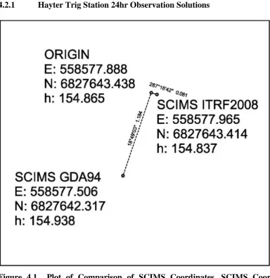
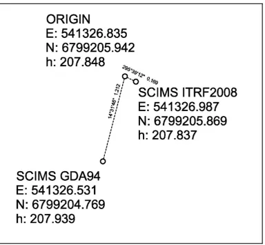
The calculated origin at Hayter Trig Station was found to be 287°18’42” for 0.081m from the average SCIMS coordinate transformed to ITRF2008 using the AUSPOS parameters (see Figure 4.2). The transformed Meerschaum Trig coordinate was found to have an even greater separation from the calculated origin with the origin being 295°39’12” for 0.169m from the average transformed coordinate (see Figure 4.4). Further investigation with LPI uncovered that the separation of the coordinates and solutions is due to the fact that AUSPOS, OPUS, CSRS and Magic all provide solutions based on the ITRF2008, independent of local control networks. SCIMS coordinates are fitted to existing control with a least squares adjustment. Baxter (2014) reported that differences between SCIMS and solutions derived from AUSPOS or CORS can typically be 0.04 m or even larger. This is due to the original GDA94 adjustment and subsequent adjustments when coordinating survey marks throughout the state. He indicates that these errors have been propagated though the network and are likely to be more pronounced in rural areas due to the greater distances. The results of this study would confirm this view and indicate that in the North Coast Region of NSW there is a substantial difference between the SCIMS coordinates and ITRF2008. As such, any solutions derived from these online service providers would require connection to the existing network if network relevance was a requirement of a particular survey.

4.2 Twenty-Four-Hour Observation Solutions

4.2.1 Hayter Trig Station 24hr Observation Solutions

Figure 4.1 Plot of Comparison of SCIMS Coordinates, SCIMS Coordinates Transformed to ITRF2008 and the Average of the Processed Solutions (Origin) at Hayter Trig Station

Figure 4.1 shows the separation between the SCIMS GDA94 coordinates, the SCIMS coordinates transformed to ITRF2008 and the average of the twenty-four hour solutions (Origin) derived from the various service providers at Hayter Trig Station.

Table 4.1 AUSPOS 24hr Observation Solutions – Hayter Trig

AUSPOS

24hr A 558577.885 6827643.440 154.866

24hr B 558577.886 6827643.441 154.854 24hr C 558577.887 6827643.440 154.871

Avg

24hr 558577.886 6827643.440 154.864

Table 4.3 CSRS 24hr Observation Solutions – Hayter Trig

CSRS

24hr A 558577.880 6827643.435 154.861 24hr B 558577.883 6827643.438 154.864

24hr C 558577.886 6827643.442 154.864

Avg

24hr 558577.883 6827643.438 154.863

Table 4.2 OPUS 24hr Observation Solutions – Hayter Trig

OPUS

24hr A 558577.884 6827643.433 154.868

24hr B 558577.886 6827643.436 154.860 24hr C 558577.882 6827643.438 154.875

Avg

24hr 558577.884 6827643.436 154.868

Table 4.4 Magic 24hr Observation Solutions – Hayter Trig

Magic

24hr A 558577.891 6827643.435 154.869 24hr B 558577.899 6827643.438 154.862

24hr C 558577.901 6827643.435 154.865

Avg

24hr 558577.897 6827643.436 154.865

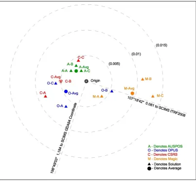
Figure 4.2 Plot of 24-hr Solutions - Hayter Trig

4.2.2 Meerschaum Trig Station 24hr Observation Solutions

Figure 4.3 Plot of Comparison of SCIMS Coords, SCIMS Coords Transformed to ITRF2008 and the Average of the Processed Solutions (Origin) at Meerschaum Trig Station

Table 4.5 AUSPOS 24hr Observation Solutions - Meerschaum Trig

AUSPOS

24hr A 541326.833 6799205.947 207.847

24hr B 541326.836 6799205.945 207.846 24hr C 541326.834 6799205.947 207.849

Avg

24hr 541326.834 6799205.946 207.847

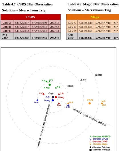
Table 4.7 CSRS 24hr Observation Solutions – Meerschaum Trig

CSRS

24hr A 541326.837 6799205.940 207.843 24hr B 541326.837 6799205.943 207.855

24hr C 541326.832 6799205.943 207.841

Avg

24hr 541326.835 6799205.942 207.846

Table 4.6 OPUS 24hr Observation Solutions – Meerschaum Trig

OPUS

24hr A 541326.830 6799205.941 207.853

24hr B 541326.840 6799205.939 207.858 24hr C 541326.835 6799205.942 207.848

Avg

24hr 541326.835 6799205.941 207.853

Table 4.8 Magic 24hr Observation Solutions – Meerschaum Trig

Magic

24hr A 541326.840 6799205.940 207.845 24hr B 541326.851 6799205.940 207.851

24hr C 541326.851 6799205.940 207.845

Avg

24hr 541326.847 6799205.940 207.847

A similar result is seen with the solutions for Meerschaum Trig Station to those observed at Hayter Trig Station. The easting coordinates are within 21mm, northing coordinates within 8mm and ellipsoidal heights within 17mm. As illustrated in Figure 4.4, the Magic solutions are biased to the east, the AUSPOS solutions biased to the North and OPUS solutions biased to the south. The CSRS solutions however, are plotted around the origin all within 3mm .

4.3 Solutions by Observation Length

4.3.1 Residuals by observation length

Tables 4.9 and 4.10 include the residuals of solutions from the calculated origin for each observation length. These will be utilised in Chapter 5 to undertake statistical analysis to examine precision and accuracy of the solutions as observation time increases.

Table 4.9 Residuals by Observation Length - Hayter Trig Station

AUSPOS OPUS CSRS-PPP MAGIC-GNSS

∆E ∆N ∆h ∆E ∆N ∆h ∆E ∆N ∆h ∆E ∆N ∆h

1hr A -0.029 -0.026 0.127 * -0.016 0.012 -0.021 -0.013 0.012 0.055 2hr A -0.001 0.007 0.012 * -0.010 0.003 -0.008 -0.002 -0.001 0.034 4hr A -0.001 0.005 0.012 -0.007 -0.005 0.017 -0.005 0.003 -0.006 0.001 0.003 0.010 6hr A -0.001 0.004 0.007 -0.005 -0.002 0.013 -0.005 0.003 0.000 0.003 -0.001 0.013 8hr A -0.001 0.004 0.007 -0.004 -0.001 0.013 -0.008 0.003 0.005 0.006 -0.001 0.011 12hr A 0.000 0.004 0.000 -0.003 -0.001 0.007 -0.005 0.003 -0.004 0.006 -0.001 0.012 24hr A 0.000 0.004 0.000 -0.001 -0.003 0.002 -0.005 -0.001 -0.005 0.006 -0.001 0.003

1hr B 0.003 -0.003 -0.017 * -0.028 0.004 0.064 -0.012 0.001 0.029 2hr B -0.007 -0.002 0.028 -0.015 -0.025 0.004 -0.025 0.004 0.034 -0.001 0.001 0.022 4hr B -0.004 0.003 0.004 -0.010 0.000 0.018 -0.017 0.004 0.010 0.002 0.004 0.009 6hr B -0.003 0.002 -0.002 -0.006 -0.001 0.010 -0.014 0.004 0.003 0.002 0.001 0.009 8hr B -0.002 0.002 -0.006 -0.005 -0.001 0.008 -0.006 0.000 -0.001 0.007 -0.003 0.007 12hr B -0.001 0.002 -0.012 -0.005 -0.001 -0.003 -0.006 0.004 -0.003 0.007 0.000 0.005 24hr B -0.003 0.003 -0.006 -0.003 -0.002 0.000 -0.006 0.000 0.004 0.010 0.000 0.002

1hr C -0.010 0.000 0.006 * -0.020 0.003 0.003 0.018 -0.001 -0.005 2hr C -0.002 0.003 0.002 -0.006 0.002 0.002 -0.012 0.003 0.001 0.029 -0.001 -0.011 4hr C -0.005 0.000 0.005 -0.008 0.000 0.005 -0.009 0.003 0.005 0.016 -0.004 -0.006 6hr C -0.005 0.002 0.010 -0.009 -0.001 0.008 -0.014 0.003 0.010 0.007 -0.004 0.001 8hr C -0.004 0.002 0.009 -0.008 0.000 0.011 -0.012 0.003 0.009 0.010 -0.004 -0.002 12hr C -0.002 0.001 -0.002 -0.006 -0.001 0.005 -0.003 0.003 -0.004 0.000 -0.004 0.000 24hr C -0.002 0.001 0.002 -0.007 -0.001 0.006 -0.003 0.003 -0.005 0.012 -0.004 -0.004

Table 4.10 Residuals by Observation Length - Meerschaum Trig Station

AUSPOS OPUS CSRS-PPP MAGIC-GNSS

∆E ∆N ∆h ∆E ∆N ∆h ∆E ∆N ∆h ∆E ∆N ∆h

1hr A -0.006 0.004 -0.007 * -0.017 0.001 -0.003 0.005 0.004 -0.012 2hr A -0.008 0.003 0.012 -0.015 -0.004 0.013 -0.022 0.001 0.022 0.002 0.005 0.003 4hr A -0.005 0.005 -0.009 -0.008 0.000 -0.011 -0.014 0.001 0.004 0.005 0.001 -0.017 6hr A -0.003 0.005 0.002 -0.005 0.002 -0.003 -0.009 0.001 0.002 0.008 -0.002 -0.020 8hr A -0.002 0.004 -0.001 -0.005 0.000 -0.004 -0.003 0.001 -0.006 0.005 -0.002 -0.019 12hr A -0.002 0.005 -0.005 -0.005 -0.001 0.001 0.002 0.001 -0.012 0.005 -0.002 -0.004 24hr A -0.002 0.005 0.000 -0.005 -0.001 0.006 0.002 0.001 -0.012 0.005 -0.002 -0.002

1hr B -0.010 -0.005 0.011 * -0.023 0.005 0.001 0.015 0.008 -0.029 2hr B -0.007 0.001 -0.003 -0.010 0.000 0.002 -0.007 0.001 -0.012 0.018 0.004 -0.029 4hr B -0.005 -0.001 -0.012 -0.010 -0.003 -0.001 -0.009 0.001 -0.016 -0.001 0.001 -0.011 6hr B -0.005 0.000 -0.015 -0.008 -0.007 0.003 -0.004 0.001 -0.015 0.007 -0.002 -0.006 8hr B -0.003 0.001 -0.016 -0.008 -0.003 0.003 -0.001 0.001 -0.015 0.010 -0.002 -0.001 12hr B -0.004 0.002 -0.018 -0.008 -0.003 0.003 -0.004 0.001 -0.011 0.010 -0.002 0.000 24hr B -0.005 0.003 -0.007 -0.001 -0.003 0.005 -0.004 0.001 0.002 0.010 -0.002 -0.002

1hr C 0.000 0.005 -0.015 * -0.012 0.003 -0.008 0.029 -0.003 -0.019 2hr C -0.002 0.004 -0.003 -0.002 0.001 0.000 -0.006 0.003 0.002 0.010 -0.003 -0.005 4hr C -0.004 0.004 0.000 -0.008 0.001 0.006 -0.006 0.003 0.005 0.013 -0.003 0.001 6hr C -0.004 0.004 0.003 -0.007 0.002 0.009 -0.012 0.003 0.013 0.010 -0.006 0.002 8hr C -0.004 0.004 0.000 -0.006 0.001 0.004 -0.006 0.003 0.008 0.010 -0.006 0.002 12hr C -0.004 0.004 -0.002 -0.008 0.000 0.004 -0.004 0.000 -0.004 0.010 -0.006 0.007 24hr C -0.004 0.004 0.003 -0.003 -0.001 0.002 -0.006 0.000 -0.005 0.013 -0.003 -0.001

As can be seen in Tables 4.9 and 4.10 the one-hour observation residuals are typically greater than those from the two-hour files and longer. This was expected as AUSPOS issues a caution with their report stating that ambiguities have not been resolved for the one-hour solution. CSRS shows the 95% confidence interval of the solution to be in the order of 25mm 40m and 82mm in E, N, and ellipsoidal height respectively. Opus will not process one-hour files in this region but provides a percentage of ambiguities resolved in the longer observation solutions (which increase as observation length increases) and Magic does not provide any specific cautionary statement.

It is possible that a large proportion of the error in the one-hour solutions is attributable to ambiguity. However the relatively larger residuals seen at Hayter Trig Station in session A may be attributable to some other source. Investigation into the processing method did not identify any external source of error with regards to incorrect instrument heights, data entry error or any other source of human error associated with data processing. Data was processed a second time to check for anomalies with no change in solution. Crawford (2013, pp. 146-147) examined the effects of a seagull or similar sized bird sitting on a receiver antenna. He found that there was more pronounced height variation and an increase in noise in the solution. He found that the standard deviation of the heights at least doubled and the amplification of noise was by a factor of 3 at the minimum and 6 at the maximum. The presence of bird faeces was discovered on the antenna after the session so this may account for the unusual results but cannot be confirmed. Also, solar activity could play a part but since session A was not conducted concurrently for both trig stations, the data cannot be compared for similar distortions or anomalies.

4.4 Solution by Data Type

Table 4.11 Comparison of 24hr GPS and GNSS Solutions - Hayter Trig Station

CSRS-PPP MAGIC-GNSS

E N h E N h

GPS A 558577.886 6827643.442 154.859 558577.891 6827643.435 154.867

GPS B 558577.877 6827643.439 154.857 558577.894 6827643.439 154.855

GPS C 558577.885 6826143.442 154.869 558577.896 6827643.432 154.864

Avg GPS 558577.883 6827143.441 154.862 558577.894 6827643.435 154.862 GNSS A 558577.880 6827643.435 154.861 558577.891 6827643.435 154.869 GNSS B 558577.883 6827643.438 154.864 558577.899 6827643.438 154.862 GNSS C 558577.886 6827643.442 154.864 558577.901 6827643.435 154.865 Avg GNSS 558577.883 6827643.438 154.863 558577.897 6827643.436 154.865

The CSRS solutions at Hayter Trig show the range of GPS coordinates to be within 9mm in easting, 3mm in northing and 12mm in height. For GNSS coordinates, the ranges are within 6mm in easting, 7mm in northing and 3mm in height. For Magic solutions, the range of GPS coordinates is within 5mm in easting, 7mm in northing and 12mm in height. For the GNSS coordinates, 10mm in easting, 3mm in northing and 7mm in height.

Table 4.12 Comparison of 24hr GPS and GNSS Solutions - Meerschaum Trig Station

CSRS-PPP MAGIC-GNSS

E N h E N h

GPS A 541326.837 6799205.943 207.843 541326.837 6799205.937 207.844

GPS B 541326.834 6799205.943 207.857 541326.851 6799205.940 207.851

GPS C 541326.834 6799205.943 207.837 541326.848 6799205.937 207.843

Avg GPS 541326.835 6799205.943 207.846 541326.845 6799205.938 207.846 GNSS A 541326.837 6799205.940 207.843 541326.840 6799205.940 207.845 GNSS B 541326.837 6799205.943 207.855 541326.851 6799205.940 207.851 GNSS C 541326.832 6799205.943 207.841 541326.851 6799205.940 207.845 Avg GNSS 541326.836 6799205.942 207.846 541326.847 6799205.940 207.847

The CSRS solutions at Meerschaum Trig show the range of GPS coordinates to be within 3mm in easting, 0mm in northing and 20mm in height. For GNSS coordinates, the ranges are within 5mm in easting, 3mm in northing and 14mm in height. For Magic solutions, the range of GPS coordinates is within 14mm in easting, 3mm in northing and 8mm in height. For the GNSS coordinates, 11mm in easting, 0mm in northing and 4mm in height.

appears to be similar at Meerschaum Trig, the GPS solutions are slightly more precise. The accuracy and precision of the other solutions at each trig station don’t appear to be noticeably more accurate or precise. The data will be statistically analysed in the next chapter to more closely inspect performance.

Figure 4.6 Plot of GPS vs GNSS Solutions – Meerschaum Trig

4.5 Summary

CHAPTER 5 – DATA ANALYSIS

5.1 Introduction

The Aim of this chapter will be to give meaning to the results of data capture and statistical analysis. At the conclusion of this chapter the reader should have an understanding of the performance of the respective service providers and the suitability for their use in the North Coast region of NSW. It should provide greater understanding of the bias observed in the results in Chapter 4 and to what extent this affects accuracy and precision. It should also provide some comparison with previous studies and contribute to the weight of those findings.

In order to achieve this, solutions from each service provider presented in Chapter 4 will be statistically analysed and a variety of comparisons made in order to compare performance. Specifically these will include the examination of solutions over observation length, the comparison of differential baseline services to PPP services and the comparison of GPS derived solutions to GNSS derived solutions. Also, comparisons will be made between results of this study and those of previous studies in order to address some of the conflicting findings.

At the conclusion of this chapter, the reader should have an understanding of the performance characteristics of each service provider relative to one another and to the calculated “truth”.

5.2 Three-Hour Solution Comparison

5.2.1 Residuals

Residuals were calculated for each solution from each service provider and the averages determined. The maximum and minimum residuals were determined from the sample data, the sample standard deviation of each service provider was calculated followed by the 95% confidence figure. From this, the upper and lower bounds of the confidence interval were determined for each service provider and this data plotted in graphs in order to make a determination about accuracy and precision.

Tables C1 & C2 in Appendix C present the three-hour residuals for each service provider, for each survey session, at each site. It is important to note that these residuals are calculated against the origin, the calculated “truth” for each site as explained in Chapter 4 above.

Figures 5.1 and 5.2 are plots of the 95% confidence intervals for the residuals incorporating the average solution as well as the range of residuals observed. The horizontal bars in the centre of each column represent the combined average residual for each coordinate element. The closer this bar is to zero the more accurate the solution relative to the calculated origin. The coloured columns represent the spread of 95% confidence intervals and the whiskers above and below the columns represent the range of residuals. The smaller the columns, the smaller the 95% confidence interval and thus the more precise the solution. The smaller the whiskers, the closer the solutions are to the real solution (ie the smaller the variations of solutions from the real solution).

Figure 5.1 95% Confidence Interval of Residuals - Differential Baseline Solutions

Figure 5.2 95% Confidence Interval of Residuals - PPP Solutions

5.2.2 Repeatability

When analysing repeatability, we are aiming to test the ability of each service provider to repeatedly process data from the same location and produce the same or similar results each time an observation session is conducted. By looking at the twenty-four-hour observation solutions and the three-twenty-four-hour residuals, we can conclude that the AUSPOS service provides a very reliable and repeatable solution. The range of coordinate differences for the twenty-four-hour solutions is shown in table 5.3 below.

Table 5.1 Solution Residuals

Service Provider Survey Site ∆E ∆N ∆h

AUSPOS Hayter 0.002 0.001 0.017

Meerschaum 0.003 0.002 0.003

OPUS Hayter 0.004 0.005 0.015

Meerschaum 0.010 0.003 0.010

CSRS Hayter 0.006 0.007 0.003

Meerschaum 0.005 0.003 0.014

Magic Hayter 0.010 0.003 0.007

Meerschaum 0.011 0.000 0.006

Figures 5.1 and 5.2 show that repeatability at 95% confidence is in the order of 15mm for AUSPOS for position and 40mm for height, OPUS shows 40mm for position and 80mm for height, CSRS shows 45mm for position and 65mm for height and Magic shows 40mm for position and 80mm for height

5.3 Differential Baseline vs PPP

In this section the solutions are combined according to processing method in order to ascertain the performance of differential baseline processing against true PPP processing.

Figure 5.3 Combined 95% Confidence Interval of Residuals – Differential Baseline vs PPP

When the solutions are combined according to processing method, it can be seen that the differential method shows a better level of precision than PPP in horizontal components but only slightly better in the height component. The spread of the height residuals is similar but PPP is trending to a height lower than the average whilst the differential solutions are trending towards a height greater than the average.

5.4 GPS vs GNSS

Table 5.2 GPS Average Solutions - 3hr Residuals GPS

Solution

CSRS-GPS MAGIC - GPS

∆E ∆N ∆h ∆E ∆N ∆h

Avg -0.007 0.006 -0.001 0.009 -0.002 -0.007

Table 5.3 GNSS Average Solutions - 3hr Residuals GNSS

Solution

CSRS-GNSS MAGIC-GNSS

∆E ∆N ∆h ∆E ∆N ∆h

Avg -0.006 0.003 0.000 0.010 -0.001 -0.002

Table 5.2 presents the average three-hour residuals for CSRS and Magic Solutions derived from GPS only data. Table 5.3 presents the average three-hour residuals for GNSS data. Tables C1, C2 and C3 in Appendix C provide a full list of the three-hour residuals. These are used in the preparation of the graphs below. Figures 5.4, 5.5 and 5.6 graph the comparison of the 95% confidence intervals of the residuals.

Figure 5.4 95% Confidence Interval of Residuals - CSRS GPS vs CSRS GNSS

The comparison of CSRS GPS and GNSS solutions indicates a slightly better precision with the GNSS based solutions. The accuracy of solutions compared to the calculated origin is very similar.

Figure 5.5 95% Confidence Interval of Residuals – Magic GPS vs Magic GNSS

The magic solutions reflect that of the CSRS solutions. The horizontal GNSS coordinates are more precise than the GPS coordinates however the height component is less precise with the GNSS coordinate and shows a much greater spread of the outliers.

When the respective solutions are combined according to data type (see Figure 5.6), it is clear to see that the GNSS based solutions offer a more precise alternative for horizontal position. With regards to height, the GNSS solutions offer a slightly better precision and slightly lesser spread of the outliers.

R

esi

d

u

al

(

m)

R

esi

d

u

al

(

Figure 5.6 95% Confidence Intervals of Residuals – Combined GPS vs Combined GNSS

When comparing this data to the conclusion of Cai & Gao (2012) there is an interesting finding. Their study compared GPS to GLONASS solutions and determined GPS provided more accurate results, most likely due to the better availability of the GPS constellation. This study has combined GPS and GLONASS data for comparison with GPS only data and found that this provides a similar accuracy with