High-Dimensional Linear and Functional Analysis of Multivariate Grapevine Data

(1)

Theses Thesis/Dissertation Collections

5-19-2017

High-Dimensional Linear and Functional Analysis

of Multivariate Grapevine Data

Follow this and additional works at:http://scholarworks.rit.edu/theses

This Thesis is brought to you for free and open access by the Thesis/Dissertation Collections at RIT Scholar Works. It has been accepted for inclusion in Theses by an authorized administrator of RIT Scholar Works. For more information, please [email protected].

Recommended Citation

(2)

ROCHESTER INSTITUTE OF TECHNOLOGY

High-Dimensional Linear and Functional

Analysis of Multivariate Grapevine Data

Author:

Supervisor:

Uday Kant Jha

Dr. Peter Bajorski

A thesis submitted in partial fulfillment of the requirements for the degree of

Master of Science in Applied Statistics

in the

School of Mathematical Sciences

College of Science

(3)

Declaration of Authorship

I, Uday Kant Jha, declare that this thesis titled, “High-Dimensional Linear and Functional Analysis

Of Multivariate Grapevine Data” and the work presented in it are my own. I confirm that:

• This work was done wholly or mainly while in candidature for a research degree at

this University.

• Where any part of this thesis has previously been submitted for a degree or any other

qualification at this University or any other institution, this has been clearly stated.

• Where I have consulted the published work of others, this is always clearly attributed.

• Where I have quoted from the work of others, the source is always given. Except for

such quotations, this thesis is entirely my work.

• I have acknowledged all main sources of help.

• Where the thesis is based on work done by myself jointly with others, I have made clear exactly what was done by others and what I have contributed myself.

Signed:

(4)

CERTIFICATE OF APPROVAL

The thesis titled “High-Dimensional Linear and Functional Analysis of Multivariate Grapevine

Data” by Uday Kant Jha, a candidate for the degree of Master of Science in Applied Statistics

has been examined and approved as worthy of acceptance.

_____________________________________________________________________________

Dr. Peter Bajorski, Professor, School of Mathematical Sciences Date

Thesis Advisor

_____________________________________________________________________________

Dr. Jan van Aardt, Professor, Center for Imaging Science Date

Committee Member

_____________________________________________________________________________

Dr.Ernest Fokoué, Associate Professor, School of Mathematical Sciences Date

(5)

ROCHESTER INSTITUTE OF TECHNOLOGY

Abstract

By Uday Kant Jha

School of Mathematical Sciences

Master of Science in Applied Statistics

Variable selection plays a major role in multivariate high-dimensional statistical modeling.

Hence, we need to select a consistent model, which avoids overfitting in prediction, enhances

model interpretability and identifies relevant variables. We explore various continuous, nearly

unbiased, sparse and accurate technique of linear model using coefficients paths like penalized

maximum likelihood and nonconvex penalties, and iterative Sure Independence Screening (SIS).

The convex penalized (pseudo-) likelihood approach based on the elastic net uses a mixture of the ℓ1 (Lasso) and ℓ2 (ridge regression) simultaneously achieve automatic variable selection,

continuous shrinkage, and selection of the groups of correlated variables. Variable selection using

coefficients paths for minimax concave penalty (MCP), starts applying penalization at the same

rate as Lasso, and then smoothly relaxes the rate down to zero as the absolute value of the

coefficient increases. The sure screening method is based on correlation learning, which computes

component wise estimators using AIC for tuning the regularization parameter of the penalized

likelihood Lasso. To reflect the eternal nature of spectral data, we use the Functional Data approach

by approximating the finite linear combination of basis functions using B-splines. MCP, SIS and

Functional regression are based on the intuition that the predictors are independent. However,

high-dimensional grapevine dataset suffers from ill-conditioning of the covariance matrix due to

multicollinearity. Under collinearity, the Elastic-Net Regularization path via Coordinate Descent

yields the best result to control the sparsity of the model and cross-validation to reduce bias in

variable selection. Iterative stepwise multiple linear regression reduces complexity and enhances

the predictability of the model by selecting only significant predictors.

Keywords: [Variable Selection; Elastic-Net; Minimax Concave Penalty; Sure

(6)

Acknowledgements

I would first like to thank my thesis advisor Dr. Peter Bajorski for his tremendous support

and help. I learned a lot from him, and this thesis would not have been materialized without his

encouragement.

I wish to thank Dr. Jan van Aardt for his acceptance of being on my thesis committee and

providing me with the data used in this thesis.

I would also like to thank Dr. Ernest Fokoué for their acceptance of being on my thesis

committee and helping with a solution to my queries.

I would also like to thank Grant W.F. Anderson for providing me with the data used in this

thesis.

Finally, I would like to thank my parents, siblings, and family for their support and endless

(7)

List of Figures

Figure 7.1: Location of the farm for data collection………...…29

Figure 8.1: Spectral Curve measurement of the Reflectance against the wavelength…...……….33

Figure 8.2: Spectral Curve measurement of the Reflectance against the wavelength after replacing wrong observations with mean……..………34

Figure 8.3: Correlation plot of Wavelength for nitrogen….………..37

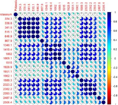
Figure 8.4: Correlation plot of Wavelength for Potassium………38

Figure 8.5: Correlation plot of Wavelength for Phosphorus……….39

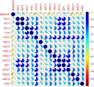
Figure 8.6: Correlation plot of Wavelength for Magnesium……….39

Figure 8.7: Correlation plot of Wavelength for Zinc………39

Figure 8.8: Correlation plot of Wavelength for Boron……….………40

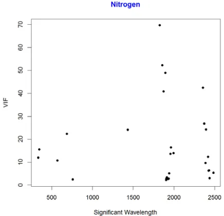
Figure 8.9: Scatterplot of VIF against Wavelength for Nitrogen………..41

Figure 8.10: Scatterplot of VIF against Wavelength for Potassium………42

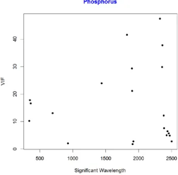
Figure 8.11: Scatterplot of VIF against Wavelength for Phosphorus……….….42

Figure 8.12: Scatterplot of VIF against Wavelength for Magnesium………..43

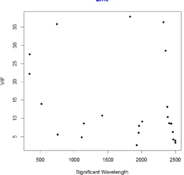
Figure 8.13: Scatterplot of VIF against Wavelength for Zinc……….43

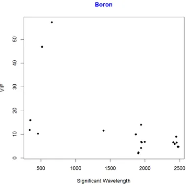
Figure 8.14: Scatterplot of VIF against Wavelength for Boron………...44

Figure 8.15: Residual Plot of Nitrogen………45

Figure 8.16: Residual Plot of Potassium……….……….45

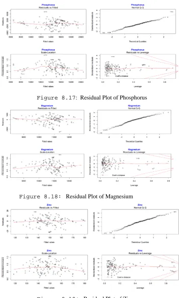
Figure 8.17: Residual Plot of Phosphorus………46

Figure 8.18: Residual Plot of Magnesium………46

Figure 8.19: Residual Plot of Zinc………46

Figure 8.20: Residual Plot of Boron……….47

Figure 9.1: Model Coefficient Path using Elastic Net for the Nitrogen……….….50

Figure 9.2: Mean-Squared Error and log (λ) using Elastic Net for the Nitrogen………51

Figure 9.3: Coefficients of Non-Zero Variables for the Nitrogen………52

Figure 9.4: Model Coefficient Path using Elastic Net for the Potassium………52

Figure 9.5: Mean-Squared Error and log (λ) using Elastic Net for the Potassium………53

Figure 9.6: Coefficients of Non-Zero Variables for the Potassium……….53

Figure 9.7: Model Coefficient Path using Elastic Net for the Phosphorus………54

Figure 9.8: Mean-Squared Error and log (λ) using Elastic Net for the Phosphorus………54

Figure 9.9: Coefficients of Non-Zero Variables for the Phosphorus………54

(11)

Figure 9.11: Mean-Squared Error and log (λ) using Elastic Net for the Magnesium………55

Figure 9.12: Coefficients of Non-Zero Variables for the Magnesium……….56

Figure 9.13: Model Coefficient Path using Elastic Net for the Zinc………56

Figure 9.14: Mean-Squared Error and log (λ) using Elastic Net for the Zinc………57

Figure 9.15: Coefficients of Non-Zero Variables for the Zinc……….……57

Figure 9.16: Model Coefficient Path using Elastic Net for the Boron………..……58

Figure 9.17: Mean-Squared Error and log (λ) using Elastic Net for the Boron……….58

Figure 9.18: Coefficients of Non-Zero Variables for the Boron………….……….58

Figure 9.19: MCP Coefficient Paths for the response variable - Nitrogen………...61

Figure 9.20: MSE and log (λ) using MCP for the response variable - Nitrogen……….…….62

Figure 9.21: R-Squared and log (λ) using MCP for the response variable - Nitrogen……….……63

Figure 9.22: MCP Coefficient Paths for the response variable - Potassium……….……63

Figure 9.23: MSE and log (λ) using MCP for the response variable - Potassium………63

Figure 9.24: R-Squared and log (λ) using MCP for the response variable - Potassium……….64

Figure 9.25: MCP Coefficient Paths for the response variable - Phosphorus………..64

Figure 9.26: MSE and log (λ) using MCP for the response variable - Phosphorus……….64

Figure 9.27: R-Squared and log (λ) using MCP for the response variable - Phosphorus………65

Figure 9.28: MCP Coefficient Paths for the response variable - Magnesium………65

Figure 9.29: MSE and log (λ) using MCP for the response variable - Magnesium……….65

Figure 9.30: R-Squared and log (λ) using MCP for the response variable - Magnesium………….……66

Figure 9.31: MCP Coefficient Paths for the response variable - Zinc……….……….66

Figure 9.32: MSE and log (λ) using MCP for the response variable - Zinc……….………66

Figure 9.33: R-Squared and log (λ) using MCP for the response variable - Zinc………67

Figure 9.34: MCP Coefficient Paths for the response variable - Boron………..….67

Figure 9.35: MSE and log (λ) using MCP for the response variable - Boron……….….67

Figure 9.36: R-Squared and log (λ) using MCP for the response variable - Boron……….68

Figure 9.37: Plot of beta coefficients for the response variable - Nitrogen……….………70

Figure 9.38: Plot of beta coefficients for the response variable - Potassium……….…71

Figure 9.39: Plot of beta coefficients for the response variable - Phosphorus………….………71

Figure 9.40: Plot of beta coefficients for the response variable - Magnesium…….………71

Figure 9.41: Plot of beta coefficients for the response variable - Zinc………72

Figure 9.42: Plot of beta coefficients for the response variable - Boron………72

Figure 9.43: Beta coefficient of response variable Nitrogen for Functional Regression………….….…74

(12)

Figure 9.45: CV of Functional Regression for response variable - Nitrogen………...75

Figure 9.46: Optimized beta function for response variable - Nitrogen………76

Figure 9.47: Beta coefficient of Functional Regression for response variable - Potassium…………...76

Figure 9.48: CV of Functional Regression for response variable - Potassium……….76

Figure 9.49: CV of Functional Regression for response variable - Potassium……….77

Figure 9.50: Optimized beta function for response variable - Potassium………...,,77

Figure 9.51: Beta coefficient of Functional Regression for response variable - Phosphorus………….,,77

Figure 9.52: CV of Functional Regression for response variable - Phosphorus………78

Figure 9.53: CV of Functional Regression for response variable - Phosphorus………78

Figure 9.54: Optimized beta function for response variable - Phosphorus………78

Figure 9.55: Beta coefficient for Functional Regression of response variable - Magnesium………79

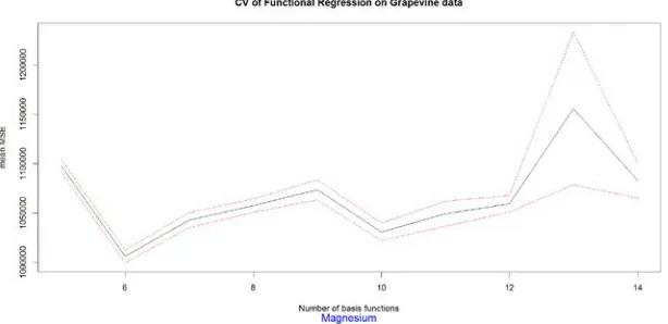
Figure 9.56: CV of Functional Regression for response variable - Magnesium………79

Figure 9.57: CV of Functional Regression for response variable - Magnesium………..79

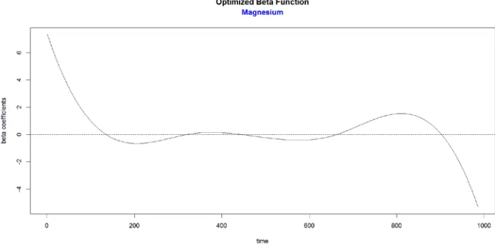
Figure 9.58: Optimized beta function for response variable - Magnesium………..…80

Figure 9.59: Beta coefficient of Functional Regression for response variable - Zinc………..…80

Figure 9.60: CV of Functional Regression for response variable - Zinc………..…81

Figure 9.61: CV of Functional Regression for response variable - Zinc………..…81

Figure 9.62: Optimized beta function for response variable - Zinc………..…81

Figure 9.63: Beta coefficient of Functional Regression for response variable - Boron………..….82

Figure 9.64: CV of Functional Regression for response variable - Boron………..…….82

Figure 9.65: CV of Functional Regression for response variable - Boron……….82

Figure 9.66: Optimized beta function for response variable - Boron……….83

Figure 10.1: Scatterplot of VIF against Wavelength - Nitrogen………86

Figure 10.2: Scatterplot of VIF against Wavelength - Potassium……….87

Figure 10.3: Scatterplot of VIF against Wavelength - Phosphorus………...…87

Figure 10.4: Scatterplot of VIF against Wavelength - Magnesium ……….…88

Figure 10.5: Scatterplot of VIF against Wavelength - Zinc………..…89

Figure 10.6: Scatterplot of VIF against Wavelength - Boron………..….89

Figure 10.7: Scatterplot of VIF against Wavelength - Nitrogen………..….90

Figure 10.8: Scatterplot of VIF against Wavelength - Potassium…...……….….…91

Figure 10.9: Scatterplot of VIF against Wavelength - Phosphorus……….……….….…92

Figure10.10: Scatterplot of VIF against Wavelength - Magnesium……..………92

Figure10.11: Scatterplot of VIF against Wavelength - Zinc……….………93

(13)

Figure10.13: Scatterplot of VIF against Wavelength - Nitrogen………94

Figure10.14: Scatterplot of VIF against Wavelength – Potassium………..95

Figure10.15: Scatterplot of VIF against Wavelength - Phosphorus………96

Figure10.16: Scatterplot of VIF against Wavelength - Magnesium……….………96

Figure10.17: Scatterplot of VIF against Wavelength - Zinc………97

Figure10.18: Scatterplot of VIF against Wavelength - Boron……….….97

Figure 11.1: Spectral Curve measurement of Riesling Bloom Petiole Analysis dataset……….101

Figure 11.2: Spectral Curve of Riesling Bloom Petiole Analysis dataset without wrong Observations………..……….…….101

Figure 11.3: Spectral Curve measurement of Riesling Bloom at Nadir dataset……….……...104

Figure 11.4: Spectral Curve of Riesling Bloom Petiole Nadir dataset without wrong observation...104

Figure 11.5: Spectral Curve measurement of CF Bloom Leaf Analysis dataset……….106

Figure 11.6: Spectral Curve measurement of CF Bloom Leaf dataset without wrong observation...106

Figure 11.7: Spectral Curve measurement of CF Bloom Leaf Analysis dataset………..108

(14)

List of Tables

Table 8.1: Max and Min correlation with the response variables of the grapevine dataset………38

Table 8.2: Median VIF of significant predictors for response variable of grapevine dataset…………....42

Table 8.3: Outliers for response variable of grapevine dataset……….45

Table 8.4: Influential cases for response variable of grapevine dataset………47

Table 9.1: Lambda values corresponding to the minimum MSE………...…...51

Table 9.2: MCP coefficient paths of response variable of the grapevine dataset………...…...61

Table 9.3: Lambda values for response variable of the grapevine dataset using MCP………..62

Table 9.4: Iterations and significant variables for response variables using SIS…...70

Table 10.1: Median VIF of significant predictors for lambda.min of 0.004………..86

Table 10.2: Median VIF of significant predictors for lambda.min of 0.003 ……….91

(15)

Chapter 1 Introduction

1.1 Background

Due to changing consumption patterns, Technavio analysts forecast the global consumption

of wine to reach more than 30 billion liters by 2020. To meet such a huge demand, the study of

vineyard leaf spectra becomes the key determinant of grape characteristics like fruit ripening rate,

water status, infestation, and disease. Macronutrients including nitrogen, phosphorus, potassium,

and magnesium, and the micronutrients including boron, and zinc are found in the soil ("Mineral

nutrients," 1998). By studying the leaf biochemistry, we can estimate the nutritional deficiencies

caused by micro and macro elements (Zarco-Tejada et al., 2005). According to G. W. Anderson

(2016) and Anderson et al. (2016), the six vital nutrients that interest the viticulturists for the

growth of wine grapes are nitrogen, potassium, phosphorous, magnesium, zinc, and boron.

Mineral Nutrition and Suppression of Plant Disease, (2014) and Mineral nutrients (1998)

explains several essential macronutrients and micronutrients are found in grape vines. Correct

amounts of nitrogen (N), as nitrate or ammonium, is necessary for the faster growth of the plant

and enhanced rate of photosynthesis. Excessive nitrogen may lead plant to lack resistance to

disease whereas its deficiency may cause underdevelopment of the plants and their leaves turn

yellow prematurely. Potassium (K) improves root growth, water, and nutrient uptake, and affect

the occurrence of a plant disease. Phosphorus (P) plays a vital role in reproduction and metabolism

of the plant. Its deficiency may lead to delayed flowering, spindly appearance and bronze-violet

pigmentation of leaves and stalks. Magnesium (Mg) is a constituent of chlorophyll. Due to its

deficiency, the leaves turn yellow or brown and may shed prematurely. Zinc (Zn) is responsible

for fruit set (flowers becoming berries); shoot elongation, pollen development, and antibiotic

production to protect the plant cells. Boron (B) is essential for growth and metabolic processes that

control plant defense. Its deficiency may reduce the yield of the vines according to G. W. Anderson

(16)

To ensure good crop quality and yield, we need to control the concentrations of these

nutrients in plants. The reflectance value of leaf is expressed between 350 – 2500 nm. Hence using

electromagnetic reflectance as the input, we can predict the chemical characteristics of these

nutrients of grapevine leaves and petioles (Ordóñez, Rodríguez-Pérez, Moreira, & Sanz, 2013).

1.2 Thesis Organization

This thesis has been broadly divided into four parts. The first part, comprising of five

chapters (chapters 2 to 6), deals with the theory of all the statistical methodologies used in this

thesis. Chapter 2 deliberates about the various aspects of exploratory data analysis, like missing

values and outliers, including robust regression and multicollinearity. Chapter 3 discusses various

aspects of variable selection and stepwise linear regression. Chapter 4 deliberates about various

regularization models using coefficients paths like Ridge, Lasso, Elastic net,Smoothly Clipped

Absolute Deviations and Minimax Concave Penalty (MCP). Chapter 5 discusses various aspects

of iterative Sure Independence Screening. Chapter 6 deliberates about different aspects of the

functional approach to variable selection, including smoothing by basis representation and

validation. The second part deals with the reflectance data of the leaves of Riesling, and Cabernet

Franc variety of grapes collected from different view angle during their bloom and veraison period

of growth. The third part comprising of three chapters (chapter 8 to 10) and deals with the data

analysis of one of the various grapevine datasets. In chapter 8, exploratory data analysis is

performed on the above-selected data. In chapter 9, selection of variables is carried out using

coefficients paths, iterative sure independence screening and functional approach to obtain

optimum values of adjusted R–Squared and predicted R–Squared. Then the value of R–Squared,

adjusted R–Squared and predicted R–Squared, obtained from various methods, are compared for

further study. Chapter 10 explains the problem of dealing with multivariate data. The last part;

consist of two chapters (chapter 11 and 12). In chapter 11, four grapevine datasets are chosen from

various combinations ensuring representation of each of the two varieties, growth periods, and

view angle and analysis of leaf and petiole of the grapevine. Then these datasets are compared

based on the best method of variable selection obtained from part three. Chapter 12 provides the

(17)

Chapter 2 Exploratory Data Analysis

2.1 Introduction

The quality of a large real-world data set depends on various issues. The source of the data

is the essential factor. Data entry and acquisition is inherently prone to errors, both noncomplex

and complex. The field error rates in the data acquisition phase are typically around 5% or more

even when the most sophisticated measures to prevent error are used. Recent studies have shown

that as much as 40% of the collected data have some or other problem (Maimon & Rokach, 2005).

Therefore, for existing data sets the logical solution is to explore the dataset for possible problems

and attempt to correct the errors. To enhance the data reliability, data cleansing, such as handling

missing values and removal of noise or outliers, becomes necessary. Hence, exploratory data

analysis can be regarded as a first step, or a preprocessing step, for any data analysis.

2.2 Missing Values

To find some attribute values missing in much real-life data is ubiquitous in modern

research. Missing values is a problem because nearly all standard statistical methods presume

complete information for all the variables included in the analysis. A few missing values on some

variables can dramatically shrink the sample size, and if some important attributes missing, then

the entire study may fail. There is a variety of reasons why data sets are affected by missing

attribute values. Some attribute values were not recorded because they are considered irrelevant,

forgotten or placed into the table but later on mistakenly erased. Dealing with missing values

requires a careful examination of the data to identify the type and pattern of missing values.

Missing data can introduce bias in the parameter estimation. Hence, a suitable method should make

that bias as small as possible. The most common approach to handling such missing attribute

(18)

techniques based on replacing a missing attribute value by the most common value of that attribute,

deleting observations with missing attribute values, mean for numerical attributes or value taken

from the closest fit case.

2.3 Outliers

In the real datasets, it often happens that some observations, called outliers, are different

from the majority. These outliers may be errors, or they could have been recorded under

exceptional circumstances, or belong to another population. Hence the first steps towards finding

a coherent analysis are the detection of outliers. Although outliers are often considered as an error

or noise, they may include relevant information. Detected outliers are candidates for abnormal data

that may otherwise adversely lead to model misspecification, biased parameter estimation, and

incorrect results. It is, therefore, important to identify them before modeling and analysis. Hawkins

defines an outlier as an observation that deviates so much from other observations as to arouse

suspicion that a different mechanism generated it. For a field fi in a record, rj can be considered as

an outlier if the value of fi > μi + ε σi or the value of fi < μi - ε σi. Where μi is the mean for the field

fi, σi is the standard deviation, and ε is a user defined factor. Regardless of the distribution of the

field fi, most values should be within a certain number ε of standard deviations from the mean. The

value of ε can be user-defined, based on some domain or data knowledge (Maimon & Rokach,

2005).

There are numerous modeling methods, which are resistant to outliers or reduce their

impact. In the classical least squares (LS) method, which is acutely sensitive to regression outliers,

one often tries to detect outliers and replaces them with mean or median. At times, these outliers

may contain some useful information; hence, removing or replacing all of them with mean or

median may fail to capture the correct pattern. Hence, we need to strike a balance between

(19)

2.4 Robust Regression

In high dimensional data, the occurrence of outliers is expected, and these outliers may

receive considerably more weight leading to distorted estimates of regression coefficients. This

distortion makes detection of deviated observations (outliers) difficult because their residuals are

much smaller than they would otherwise be without distortion. Also, multivariate leverage outliers

can be masked by the effect of good leverage points, on the other hand, some good data points

might even appear to be outliers, which is known as swamping. To avoid these effects, robust

regression down weights the influence of outliers, which makes their residuals larger and easier to

identify. A robust measure is the median of all absolute deviations from the median (MAD):

MAD = 1.483 median_𝑖𝑖=1_,…,_𝑛𝑛 |𝑥𝑥𝑖𝑖− median_𝑖𝑖=1_,…,_𝑛𝑛 (𝑥𝑥𝑖𝑖)|

A correction factor, constant of 1.483 is used to make the MAD unbiased at the normal

distribution. The smallest fraction of outliers called breakdown point that may cause an estimator

to take on arbitrarily large aberrant value is around 50% for most of the robust regression method.

In other words, robust regression can provide resistant results in the presence of outliers

Rousseeuw & Hubert (2011).

2.5 Robust Regression Methods

Linear regression analysis uses the least squares, which would not be appropriate in solving

a problem containing outliers or extreme observations. Therefore, we need a parameter estimation

method, which is robust where the value of the estimation is not much affected by small deviations

in the data. The robust regression applies numerous methods to restrict the influence of outliers;

robust regression uses numerous methods. Least Trimmed Squares (LTS) estimation,

M-estimation, S-estimation and MM estimation will be explained in robust regression to determine a

regression model.

Rousseeuw & Hubert (2011) developed Least Trimmed Squares (LTS) estimation method

(20)

𝛽𝛽̂𝐿𝐿𝐿𝐿𝐿𝐿 = argmin_𝛽𝛽 �(𝑦𝑦𝑖𝑖 − 𝑥𝑥𝑖𝑖𝐿𝐿𝛽𝛽)2 ℎ

𝑖𝑖=1

= argmin_𝛽𝛽 � ϵ𝑖𝑖2 ℎ

𝑖𝑖=1

where ϵ₁2 ≤ ϵ₂2 ≤ . . . ≤ ϵ_𝑛𝑛2, are the ordered squared residuals from smallest to largest and i = 1, 2,

…, n. LTS is calculated by minimizing the h ordered squares residuals, where h= [n/2]+[(p+1)/2],

with n and p being sample size and number of parameters, respectively. The largest squared

residuals are excluded from the summation in this method, which allows those outlier data points

to be excluded completely.

The most common method of robust regression is M-estimation, introduced by Huber. Here

M indicates an estimation of the maximum likelihood type (Alma, 2011). The M-estimation

principle is to minimize the sum of a chosen function ρ of the errors, rather than minimizing the

sum of squared errors. The M-estimate objective function is,

𝛽𝛽̂𝑀𝑀 = argmin_𝛽𝛽 � 𝜌𝜌�𝑦𝑦𝑖𝑖− 𝑥𝑥𝑖𝑖 𝐿𝐿_{𝛽𝛽̂�}

𝜎𝜎�

𝑛𝑛

𝑖𝑖=1

where 𝜌𝜌 is a symmetric function and continuously differentiable with a unique minimum at zero

and 𝜎𝜎� is an estimator. An estimate of 𝜎𝜎� is given by

𝜎𝜎�=𝑚𝑚𝑚𝑚𝑚𝑚𝑚𝑚𝑚𝑚𝑚𝑚|𝜖𝜖_0.6745𝑖𝑖− 𝑚𝑚𝑚𝑚𝑚𝑚𝑚𝑚𝑚𝑚𝑚𝑚(𝜖𝜖𝑖𝑖)|

Iteratively reweighted least squares (IRLS) is used in the calculation of M-estimates. In

IRLS, the first fit is calculated, and then a new set of weights is computed based on the results of

the original fit. The iterations are continued until a specified number of iterations are finished, or

a convergence criterion is met. Thus, function ρ gives the contribution of each residual. However,

M-estimation lacks the consideration of the data distribution and uses only the median as the

weighted value; hence, it is not a function of the overall data.

To overcome the weaknesses of media, Rousseeuw & Hubert (2011) introduced a high

breakdown value method, called S-estimation. Here S indicates that it is based on estimates of

scale. S-estimators minimize the dispersion of the residuals, in the same way, that the least squares

estimator minimizes the variance of the residuals. Since the S estimate satisfies the necessary

(21)

objective function is minimized residual standard deviation 𝜎𝜎�_𝑠𝑠 (∊1(β),...,∊n(β)), where ∊i (β) is the

ith error term dependent on the regression coefficients β. 𝛽𝛽̂𝐿𝐿 = 𝑚𝑚𝑚𝑚𝑚𝑚 � 𝜌𝜌�𝑦𝑦𝑖𝑖 − 𝑥𝑥𝑖𝑖

𝐿𝐿_{𝛽𝛽̂�}

𝜎𝜎�𝑠𝑠 𝑛𝑛

𝑖𝑖=1

where 𝜌𝜌 is a symmetric function and continuously differentiable with a unique minimum at zero

and 𝜎𝜎�_𝑠𝑠 is a robust scale estimator. An estimate of 𝜎𝜎�_𝑠𝑠 is given by

𝜎𝜎�𝑠𝑠 =𝑚𝑚𝑚𝑚𝑚𝑚𝑚𝑚𝑚𝑚𝑚𝑚|𝜖𝜖_0.6745𝑖𝑖 − 𝑚𝑚𝑚𝑚𝑚𝑚𝑚𝑚𝑚𝑚𝑚𝑚(𝜖𝜖𝑖𝑖)|

MM estimation is a particular type of M-estimation with an aim to obtain estimates that

have a high breakdown value and more efficient. Yohai (1987) developed the MM-estimates as a

three-stage procedure. In the first stage, an initial regression parameter is computed using

S-estimator, which is consistent, and robust with high breakdown point, but not necessarily efficient.

In the second stage, a more efficient M-estimate of the errors scale is computed using

residuals based on the initial estimate. The objective function used in this phase is labeled ρ0.

Finally, in the third stage, an M-estimate of the regression parameters based on a proper

redescending the Psi-function is computed. The last step computes the MM estimate of scale as

the solution to

𝛽𝛽̂𝑀𝑀𝑀𝑀 = argmin_𝛽𝛽 � 𝜌𝜌 �𝑦𝑦𝑖𝑖 − 𝑥𝑥𝑖𝑖 𝐿𝐿_𝛽𝛽̂

𝜎𝜎�𝑀𝑀𝑀𝑀 � 𝑛𝑛

𝑖𝑖=1

where 𝜎𝜎�_{𝑀𝑀𝑀𝑀} is the standard deviation obtained from the residual of S estimation.

2.6 Multicollinearity

In multiple regression models, multicollinearity (also collinearity) refers to a phenomenon

in which two or more predictors are highly correlated with each other or the response variable. It

increases the variance of the coefficient estimates and makes the estimates very sensitive to minor

(22)

In other words, by overinflating the standard errors, multicollinearity makes some variables

statistically insignificant when they should be significant.

To fit the model Y = X𝛽𝛽 + ∊. The LS solution b = (XT_X)-1 _XT_Y_{would usually be sought.}

However, if XT_X_{is singular, we cannot perform the inversion and the normal equations will not}

have a unique solution. In this situation, at least one column of X is linearly dependent on the other

columns (i.e., linear combination of the columns of the X matrix is zero). We would assume

"multicollinearity" when there exists a "near dependence" in the X columns (Draper & Smith,

1998). Multicollinearity can be reduced by removing one of the correlated predictors from the

model, because they supply redundant information.

In addition to removing correlated predictors, multicollinearity can be dealt by using other

methods, like an elastic net and functional data analysis. The elastic net can select clusters of

correlated features when the groups are not known in advance by inducing a grouping or clustering

effect during variable selection. These groups of highly correlated variables tend to have

coefficients of similar magnitude.

2.7 Variable Selection

Variable selection in multivariate analysis is a critical step in regression, especially when

the number of covariates is large in comparison to the sample size. It is an essential step because

the removal of non-informative variables will produce better prediction results with simpler

models. Hence, the selection methods are based on judicious selection of a subset of variables from

the original set, which will allow easier interpretation, better prediction, and reduction in the

complexity of the model. Penalized likelihood estimation of the coefficients, based on continuous

penalty functions, provide an attractive approach to performing variable selection and estimation

of regression coefficient by simultaneously identifying a subset of variables that are associated

with a response. In the next three chapters, we discuss various continuous, nearly unbiased, sparse

and accurate methods of variable selection using coefficients paths like penalized maximum

(23)

and their combination. Also, we discuss the iterative Sure Independence Screening and application

(24)

Chapter 3 Methods of Variable Selection

Traditional multivariate data analytical approaches assume the data of large sample size (n)

with a few predictors (p). With the amazing development of modern technology, including

computing power and storage, higher dimensional (n ‹‹ p) and high-throughput data of vast size

and complexity are being produced for contemporary statistical studies. To perform efficient and

reliable model selection for such high-dimensional multivariate data can be challenging. Let

X1, . . . , Xp is the set of predictors, with n observations and Y be the response variable. The problem

of variable selection arises when p is enormous and a subset of X1, . . . , Xp is thought to contain

many redundant variables. In recent years, the study of such dataset with the curse of

dimensionality has received great attention from the research community. Ill-conditioning of the

variance-covariance matrix for such high-dimensional dataset renders typical multivariate data

analysis unattractive (Wu & Müller, 2010). Hence penalized likelihood procedures can provide an

attractive approach for variable selection and regression coefficient estimation by simultaneously

identifying a subset of predictors that are associated with a response. For example, Cp (Mallows,

1973), AIC (Akaike, 1974) and BIC (Schwarz, 1978) are all motivated from ℓ0 penalized likelihood

regression. ℓ0 penalty directly penalizes the number of non-zero coefficients in the model and is

intuitively suitable for the purpose of variable selection. However, there are two major limitations

in this type of penalized likelihood procedure. First, the ℓ0 penalty is not continuous at the origin

point, and hence the resulting estimators are likely to be unstable. Second, ℓ0 penalized likelihood

procedure involves an exhaustive search over all possible models; hence it is computationally

infeasible for a large number of potential covariates. Hence, we require a penalized likelihood

estimation based on continuous penalty functions, like ℓ2-norm or ℓ1-norm or mixed. Ridge

regression (Hoerl & Kennard, 1970) as a continuous shrinkage method, achieves its better

prediction performance through a bias–variance trade-off by minimizing the residual sum of

(25)

parsimonious model, for it always keeps all the predictors in the model. Hence it is not a suitable

technique for an asymptotic setup (p > n). Regularization technique like Least Absolute Shrinkage

and Selection Operator (Tibshirani, 1996) based on ℓ1-norm, can reduce dimensionality, select

variables and estimate coefficients simultaneously. However, it becomes unstable when there is

collinearity in the dataset. Hence, a regularization technique like an elastic net (Zou & Hastie,

2005), which can reduce dimensionality, selects variables and encourages a grouping effect

simultaneously, appears to be a better option.

3.2 Insight into High Dimensionality

A challenge with high dimensionality is that significant predictors can be highly correlated

with some unimportant ones, which increases with dimensionality. The maximum spurious

correlation also increases with dimensionality. Consider a situation where all the predictor variable

X1, . . . , Xp is standardized. The distribution of Z =𝚺𝚺−1/2𝐗𝐗 is spherically symmetric, X = (X1,...,Xp)T and 𝚺𝚺 = cov(X). For better understanding, of the difficulties of high dimensionality

we, need to separate the effects of the covariance matrix 𝚺𝚺 and the distribution of Z (Fan & Lv,

2008).

When dimension p is larger than sample size n, then the design matrix X is rectangular,

having more columns than rows. Hence, the matrix XT_X_{is large and singular. Due to}

dimensionality, the spurious correlation between a covariate and the response could be large. The

unimportant predictors, which are associated with significant ones (predictors), become highly

correlated with the response variable, and the population covariance matrix 𝚺𝚺 may become ill

conditioned as n grows. The minimum non-zero absolute coefficient |𝛽𝛽i | may decay with n and

fall close to the noise level.

3.3 Dimensionality Reduction

The curse of dimensionality is strongly linked with the sparseness of data in a

high-dimensional space. Dimension reduction or variable selection is an effective strategy to deal with

(26)

can be radically reduced. Now, accurate coefficient estimation can be found by using one of the

well-developed lower dimensional models. The motivation for dimensionality reduction from the

original variables is to find the wavelengths significantly responsible for the calculation of various

nutrients, rather than linear combinations of all the wavelengths.

We consider the high-dimensional setting of a linear model,

Y = X𝜷𝜷 + 𝜀𝜀

Where dimension of matrix X is n × p, regression vector 𝜷𝜷, p × 1 and response vector Y and ε

with n × 1. We denote the active set of variables by

S0 = {j; 𝜷𝜷j≠ 0, j = 1, . . . , p}

The idealistic goal is to make dimensionality reduction with an estimated sparse set of

variables

S� ⊆ {1, . . . , p} such that

|S�| < n-1

Since the data are not high dimensional anymore, one can rely on more classical techniques

such as least squares estimation for further analysis using variables from the sparse set S�.

Based on the principle of parsimony, one needs to reduce the amount of complexity in the

model while dealing with huge numbers of predictors. To select useful subsets of variables, which

may be contributing significantly to the model, we use stepwise regression based on P-values of

interest.

3.4 Variable selection

Effective variable selection can lead to parsimonious models with better prediction accuracy

and easier interpretation. Ideally, the variable selection procedure should be unbiased, sparse and

(27)

𝑦𝑦𝑖𝑖 =𝛽𝛽0+𝛽𝛽1𝑥𝑥1𝑖𝑖+⋯+𝛽𝛽𝑝𝑝𝑥𝑥𝑝𝑝𝑖𝑖+𝜖𝜖𝑖𝑖 is modelled by a linear function, where 𝑦𝑦𝑖𝑖 is the response

variable, i = 1,…, n, 𝑥𝑥_{𝑖𝑖𝑖𝑖} is the explanatory variables, j = 1, . . . ,p, 𝜖𝜖_𝑖𝑖 𝑖𝑖𝑖𝑖𝑖𝑖_~ 𝑁𝑁(0,𝜎𝜎2) are error terms

and 𝛽𝛽j’s are regression, coefficients.

Without loss of generality, we can standardize the response and each covariate with zero mean

and unit standard deviation. Hence, after removing the intercept term, the regression model

mentioned above can be rewritten as given below.

𝑦𝑦𝑖𝑖 =� 𝛽𝛽𝑖𝑖𝑥𝑥𝑖𝑖𝑖𝑖 𝑝𝑝

𝑖𝑖=1

+𝜖𝜖𝑖𝑖

With a large number of predictive variables, we often would like to determine a smaller subset

that exhibits the strongest effects. For the purpose of feature selection, we consider the penalized

least squares (LS) estimation.

= min_𝛽𝛽

𝑗𝑗 �

1

2n� �𝑦𝑦𝑖𝑖− � 𝛽𝛽𝑖𝑖𝑥𝑥𝑖𝑖𝑖𝑖

𝑝𝑝 𝑖𝑖=1 � 2 𝑛𝑛 𝑖𝑖=1

+𝜆𝜆 �p𝜆𝜆 𝑝𝑝

𝑖𝑖=1

�|βj| ��

where 𝜆𝜆 is a non-negative tuning parameter and p𝜆𝜆(∙) is a sparsity-induced penalty function that

which may not depend on 𝜆𝜆 (Geng, 2014).

The standard techniques for improving the Ordinary Least Square (OLS) estimates are best

subset selection, ridge regression, lasso and elastic net. Best subset selection provides models that

can be extremely variable because it is a discrete process either retains or drops variables from the

model. Its prediction is highly sensitive to minor changes in the dataset. Best subset selection fails,

when we have many variables because of several combinations. Ridge regression is a continuous

process that improves prediction error by shrinking large regression coefficients to reduce

overfitting. However, it fails to perform covariate selection and hence is not very useful when the

number of explanatory variables exceeds the number of observation. Because of the l1 -penalty,

Lasso does variable selection and shrinkage, thus retaining the useful techniques of ridge

regression and subset selection (Tibshirani, 1996). Hence, it is very helpful when the number of

(28)

dataset. To remedy this limitation, one can use Elastic-net regularization, which adds ridge

regression-like penalty. It allows the model to select strongly correlated variables together and

improves overall prediction accuracy when the number of a covariates is larger than the sample

size.

3.5 Stepwise multiple linear regression

In the algorithm for stepwise multiple linear regression, original variables are selected

iteratively according to their correlation with the target property. For a selected variable, a

regression coefficient is determined and tested for significance using a t-test at a critical level (e.g.,

5%). If the coefficient is found to be significant, the variable is retained, and another variable is

selected according to its partial correlation with the residuals that are obtained from the model

built with the first variable. This procedure is called forward selection. The significance of the two

regression coefficients and their association with the two retained variables are then tested again,

and the non-significant terms are eliminated from the equation (backward elimination). Forward

selection and backward elimination are alternated and repeated until no significant improvement

of the model fit can be achieved by including more variables and all regression terms that are

already selected are important (Balabin & Smirnov, 2011). In this method, each variable is studied

independently, and no consideration is given to variable interaction. The stepwise subset selection

approach increases the search space to enhance the predictability of the models. Hence it suffers

(29)

Chapter 4 The regularization models

To reduce variability and achieve a more interpretable model, we often seek a smaller subset

of relevant variables. However, searching through subsets of potential predictor variables for an

adequate smaller model can be unstable and is computationally unfeasible even of modest

dimensions. The objective of variable selection is to identify features in the dataset that are

important and discard variables with irrelevant and redundant information. Since variable selection

reduces the dimensionality of the data, it holds out the possibility of more efficient & rapid

operation of the data set. The ordinary least squares (OLS) estimates often have low bias but

significant variance. With great number predictors, we often would like to determine a smaller

subset that exhibits the strongest effects. With sparsity, feature selection can improve the accuracy

of estimation by effectively identifying the subset of significant predictors, and enhance model

interpretability with parsimonious representation. Consider a linear model with a response variable

Y, depended on p explanatory variable X ∊ℝ𝑝𝑝. For small p, proper penalty on the number of

selected variables based on the Cp, AIC, BIC or a data driven method for subset selection can be

used to obtain a good guess of the pattern. However, for large p, subset selection is not

computationally feasible, so we will have to use continuous penalized or gradient threshold

methods.

We describe here algorithms for estimation of linear models with convex penalties, including ℓ1 (the Lasso), ℓ2 (ridge regression) and combinations of the two (the elastic net). This algorithm

optimizes each parameter separately, holding all other fixed. Updates are trivial. Then it cycles

around until coefficients stabilize. This process, called cyclical coordinate descent along a

regularization path, achieves dramatic speedups over other competitors. The methods can handle

(30)

The basic linear regression model used to predict the nutrients with the regularization models

is:

Y = Xβ + ∊,

where Y=(y1,...,yn)T is the vector of observed response variable, X is n × p matrix of predictors; 𝜷𝜷

is the vector of the regression coefficients of the predictors and ∊ is the vector of the residual errors

with variance (∊) = 𝜎𝜎_𝜖𝜖2 . For simplicity, we, assume that the observed variables have been

mean-centered, so that we have no need for a constant term in the regression. In other words Xij are

standardized, such that∑𝑛𝑛_𝑖𝑖=1𝑋𝑋_{𝑖𝑖𝑖𝑖} = 0,1

𝑛𝑛∑𝑛𝑛𝑖𝑖=1𝑋𝑋𝑖𝑖𝑖𝑖2 = 1, for j = 1, . . ., p.

4.2 Ridge regression

The least square estimate suffers from the deficiency of mathematical optimization techniques

that give point estimates. To control the inflation and general instability associated with the least

square estimates, one can use ridge regression (Hoerl & Kennard, 1970). Ridge regression

performs well only when there is a subset of true coefficients that are small or zero. Ridge

regression shrinks all coefficients by a uniform (ℓ2 – norm) penalty to produce a unique solution.

In the case of k identical predictors, they each get equal coefficients with 1/kth the size, which any single predictor would get if fit alone. Ridge regression is like least squares but shrinks the

estimated coefficients towards zero. For a given response vector Y∈ℝn and a predictor matrix X

∈ℝn×p_{, the ridge regression coefficients are defined as:}

𝛽𝛽̂(ridge) _{= arg min}

𝛽𝛽𝜖𝜖ℝ𝑝𝑝 {∥ 𝐘𝐘 − 𝐗𝐗𝐗𝐗 ∥2

2₊_{𝜆𝜆 ∥ 𝐗𝐗 ∥} 2 2_}

Where ∥ 𝐘𝐘 − 𝐗𝐗𝐗𝐗 ∥₂2 =∑𝑛𝑛_𝑖𝑖=1(y_𝑖𝑖 −x_𝑖𝑖𝐿𝐿β)2 is the ℓ2 –norm (quadratic) loss function (i.e. residual

sum of squares), x_𝑖𝑖𝐿𝐿 is the ith row of X, ∥ 𝐗𝐗 ∥₂2 =∑𝑝𝑝_𝑖𝑖=1𝛽𝛽_𝑖𝑖2 is the ℓ2 –norm penalty on 𝛽𝛽, and

𝜆𝜆≥ 0 is the tuning (penalty, regularization, or complexity) parameter which regulates the strength of the penalty (linear shrinkage) by determining the relative importance of the data-dependent

empirical error and the penalty term. As 𝜆𝜆 tends to infinity, the coefficients will approach zero. In

other words, the larger the value of 𝜆𝜆, the greater is the amount of shrinkage. As the value of 𝜆𝜆 is

(31)

The intercept is assumed to be zero due to mean centering of the variables. (Schulz-Streeck, Ogutu,

& Piepho, 2012). Since ridge regression does not set the coefficients exactly to zero unless 𝜆𝜆 = ∞,

in which case all the coefficients are zero. Hence ridge regression cannot select a model with the

most relevant and predictive subset of predictors.

4.3 Least Absolute Shrinkage and Selection Operator (Lasso)

Due to the nature of the ℓ1-penalty, the lasso does both continuous shrinkage and automatic

variable selection simultaneously. Even though the prediction performance of the Lasso and Ridge

regression are similar, however, the Lasso is more appealing due to its sparse representation (Zou

& Hastie, 2005). The Lasso shrinks the magnitude of all the coefficients by a constant value and

sets them to zero if they reach that value, as in the best subset selection case. In other words, Ridge

regression shrinks all regression coefficients towards zero; the Lasso tends to give a set of zero

regression coefficients, which leads to a sparse solution. The Lasso penalty corresponds to a

Laplace prior, which expects a large number of coefficients to be zero, and only a small subset to

be nonzero. The Lasso estimator uses the ℓ1 penalized least squares criterion to obtain a sparse

solution to the following optimization problem:

β�(Lasso) _{= arg min}

𝛽𝛽𝜖𝜖ℝ𝑝𝑝 {∥ 𝐘𝐘 − 𝐗𝐗𝐗𝐗 ∥2

2₊_{𝜆𝜆 ∥ 𝐗𝐗 ∥} 1}

Where ∥ 𝐘𝐘 − 𝐗𝐗𝐗𝐗 ∥₂2 = 1

2𝑛𝑛∑𝑛𝑛𝑖𝑖=1(y𝑖𝑖−x𝑖𝑖𝐿𝐿β)2 is the ℓ2 –norm (quadratic) loss function (i.e. residual

the sum of squares), x_𝑖𝑖𝐿𝐿 is the ith row of X, ∥ 𝐗𝐗 ∥₁ =∑𝑝𝑝_𝑖𝑖=1|𝛽𝛽_𝑖𝑖| is the ℓ1 –norm penalty on 𝛽𝛽, which

induces sparsity in the solution, and 𝜆𝜆⩾0 is the tuning parameter.

The ℓ1 penalty enables the Lasso to simultaneously regularize the least squares fit and shrink

some components of β�LassoTo zero for some suitably chosen 𝜆𝜆 (Schulz-Streeck et al., 2012).

Although the Lasso has many excellent properties, it is a biased estimator and the bias for a truly

nonzero variable is about λ for large regression coefficients. It is not robust to highly correlated

predictors. It also fails to do grouped selection. If there is a group of variables among which the

pairwise correlations are very high, then the lasso tends to arbitrarily pick one variable from the

(32)

down. In addition, Lasso also restricts the number of variables that can be selected. If p>n, the

lasso selects at most n variables.

4.4 Elastic net

From the Bayesian standpoint, the ridge penalty is ideal when there are many predictor

variables with non-zero coefficients (drawn from a Gaussian distribution). The Lasso penalty, on

the other hand, corresponds to a Laplace prior that assumes many coefficients to be zero, and only

a small subset to be nonzero. The elastic net is a compromise between ridge and lasso that is robust

to extreme correlations among the predictors. The elastic net encourages a grouping or clustering

effect when strongly correlated predictors enter or exit the model together. The elastic net is mainly

useful when the number of predictors (p) is bigger than the sample size (n). The elastic net is very

helpful to analyze high dimensional data and to avoid the instability of the lasso solution paths

when pairwise correlations are very high. The elastic net uses a mixture of the ℓ1(lasso) and ℓ2

(ridge regression) penalties. It is formulated as given below:

β�(enet) _{= arg min}

𝛽𝛽𝜖𝜖ℝ𝑝𝑝 {∥ 𝐘𝐘 − 𝐗𝐗𝐗𝐗 ∥2 2₊_{𝜆𝜆𝑃𝑃}

𝛼𝛼(𝛽𝛽)}

where ∥ 𝐘𝐘 − 𝐗𝐗𝐗𝐗 ∥₂2= 1

2𝑛𝑛∑𝑛𝑛𝑖𝑖=1(y𝑖𝑖 −x𝑖𝑖𝐿𝐿β)2, and P𝛼𝛼(𝛽𝛽) is the elastic net penalty subject to

𝑃𝑃𝛼𝛼(𝛽𝛽) = (1− 𝛼𝛼) ∥ 𝐗𝐗 ∥22+𝛼𝛼 ∥ 𝐗𝐗 ∥1 =∑𝑝𝑝𝑖𝑖=1[₂1(1− 𝛼𝛼)𝛽𝛽𝑖𝑖2+α|βj|]≤ s for some s

P(𝛽𝛽) creates a useful compromise between the ridge-regression penalty (α = 0) and the

lasso penalty (α = 1). The ℓ1 part of the elastic net does automatic variable selection, while the ℓ2

part encourages grouped selection and stabilizes the solution paths with respect to random

sampling, thereby improving prediction. As α increases from zero (0) to one (1), for a given λ the

sparsity of the solution (i.e., the number of coefficients equal to zero) increases monotonically

from zero to the sparsity of the lasso solution. This penalty is particularly useful in the p ≫ n

situation, or any situation where there are many correlated predictor variables However, unlike the

(33)

4.5 Smoothly Clipped Absolute Deviations (SCAD)

It is known that the ℓ2does not satisfy the sparsity condition, and the convex ℓ1 penalty

does not meet the unbiasedness condition and the concave ℓqpenalty with 0 ≤ q < 1 does not meet

the continuity status. In other words, none of these ℓ penalties satisfies all three conditions

simultaneously. In high a dimension condition, the bias of penalized estimators can almost be

removed by choosing a constant penalty beyond a second threshold level 𝛾𝛾𝜆𝜆. Fan & Lv (2010) introduced the Smoothly Clipped Absolute Deviation (SCAD), which retains the penalization rate

(and bias) of the lasso for small coefficients, but continuously relaxes the rate of penalization as

the absolute value of the coefficient increases. The SCAD penalty is continuously differentiable

on (-∞, 0) U (0, ∞), but singular at zero with its derivatives zero outside the range [−𝛾𝛾λ, 𝛾𝛾λ]. These

results in small coefficients being set to zero, a few other coefficients being shrunk towards zero

while retaining the large coefficients as they are. Thus, SCAD can produce sparse set of solution

and approximately unbiased coefficients for large coefficients. Fan & Lv (2008) defined the

continuously differentiable penalty SCAD by

𝑝𝑝λ′(|𝛽𝛽|) = λ �𝐼𝐼(|𝛽𝛽|⩽ λ) +(γλ−₍_γ−1|β₎|)_λ+𝐼𝐼(|𝛽𝛽| >𝜆𝜆)� for some 𝛾𝛾 > 2

where 𝑝𝑝_λ′(|𝛽𝛽|) is a concave penalty with respect to |𝛽𝛽|. The authors suggested using 𝛾𝛾 = 3.7. It coincides with the Lasso until |X| = λ, then smoothly transit to a quadratic function until |X| = 𝛾𝛾𝜆𝜆,

after which it remains constant for all |X| > 𝛾𝛾𝜆𝜆. These results apply to general classes of loss and

penalty functions but do not address the uniqueness of the solution or provide methodologies for

approximating the local minimizer with the stated properties. A major cause of computational and

analytical difficulties in these studies of nearly unbiased selection methods is the non-convexity

of the minimization problem.

4.6 Minimax Concave Penalty (MCP)

The Minimax Concave Penalty (MCP) starts by applying the same rate of penalization as the

lasso, and then smoothly relaxes the penalization rate to zero as the absolute value of the coefficient

increases. The MCP relaxes the penalization rate immediately, whereas for SCAD the rate remains

(34)

Zhang (2010)defined MCP as,

𝜌𝜌(𝑡𝑡;λ) =λ ∫ �1−_γλ𝑥𝑥�

+𝑚𝑚𝑥𝑥 𝑡𝑡

0 ,

with a regularization parameter 𝛾𝛾 > 0. It minimize the maximum concavity

𝜅𝜅(𝜌𝜌)≡ 𝜅𝜅(𝜌𝜌;λ) ≡ sup

0<𝑡𝑡1<𝑡𝑡2

{𝜌𝜌̇(𝑡𝑡1;λ)− 𝜌𝜌̇(𝑡𝑡2;λ)}/(𝑡𝑡2− 𝑡𝑡1)

subject to the following unbiasedness and features selection:

𝜌𝜌̇(𝑡𝑡;𝜆𝜆) = 0 ∀𝑡𝑡 ≥ 𝛾𝛾𝜆𝜆, 𝜌𝜌̇(0+;λ) =λ.

Convexity ensures that the algorithm converges to the unique global minimum and 𝛽𝛽̂ is continuous with respect to λ, which in turn ensures good initial values, thereby reducing the number of iterations required by the algorithm. In the absence of convexity, 𝛽𝛽̂ is not necessarily

continuous with respect to the data—that is, a small change in the data may produce a large change

in the estimate. Such estimators tend to have high variance in addition to being unattractive from a logical perspective. Besides, discontinuity with respect to λ increases the difficulty of choosing a good value for the regularization parameter. The coordinate descent algorithms are also not

guaranteed to converge to a global minimum in general. However, it is not always necessary to

attain global convexity. In high-dimensional settings where p > n, global convexity is neither

possible nor relevant. In such settings, sparse solutions for which the number of nonzero

coefficients is much lower than p, we will still have stable estimates and smooth coefficient paths

in the parameter space of interest (Breheny & Huang, 2011).

MCP provides the sparse convexity to the broadest extent by minimizing the maximum

concavity. The MCP achieves 𝜅𝜅(𝜌𝜌;λ) = 1/𝛾𝛾. A larger value of its regularization parameter 𝛾𝛾 affords less unbiasedness and more concavity. For each penalty level 𝜆𝜆, the MCP provides a continuum of

penalties with the ℓ1 penalty as 𝛾𝛾⟶∞ i.e., the MCP and lasso solutions are the same, and the “ℓ0

(35)

Chapter 5 Sure Independence Screening

Variable selection plays a major role in high-dimensional statistical modeling, which

nowadays appears in many areas and is key to various scientific discoveries. For problems of high

dimensionality p, the accuracy of estimation and computational cost are two top concerns. One

popular family of feature selection methods for parametric models is based on the penalized

(pseudo-)likelihood approach. It includes the Lasso (Tibshirani, 1996), the SCAD (Fan & Li,

2001), the elastic net (Zou & Hastie, 2005), the MCP (Zhang, 2010), and related techniques.

Nevertheless, in ultrahigh dimensional statistical learning problems, these methods may not

perform well due to the concurrent challenges of computational expediency, statistical accuracy,

and algorithmic stability. Motivated by these concerns, Fan & Lv (2008) introduced the concept

of sure screening method based on correlation learning, called sure independence screening. It

reduces dimensionality from high to a moderate scale, below the sample size. As a methodological

extension, iterative sure independence screening is also proposed to enhance its finite sample

performance.

5.2 Sure Independence Screening

Consider estimating a p-vector of parameters 𝛽𝛽 from the linear model

Y=X𝛽𝛽 +∊,

where Y = (Y1, . . . , Yn)T is an n-vector of responses, X = (X1,..., Xn)T is n x p matrix, which is

independent and identically distributed. X1,..., Xn, 𝛽𝛽 = (𝛽𝛽1, . . . , 𝛽𝛽p)T is a p-vector of parameters

and ∊= (∊1, . . . , ∊n)T is an n-vector of IID random errors. When the dimension p is high, it is

(36)

response, which amounts to assuming ideally that the parameter vector 𝛽𝛽 is sparse. With sparsity,

variable selection can improve the accuracy of estimation by effectively identifying the subset of

important predictors, and enhance model interpretability with parsimonious representation.

Sparsity comes frequently with high dimensional data, which is a growing feature in many areas

of contemporary statistics. The problems arise frequently in genomics, imaging, and finance,

where the number of variables or parameters p are much larger than sample size n. Let us assume

that the predictors X1, . . . , Xp are independent and follow the standard normal distribution. Then,

the design matrix is an n x p random matrix, each entry an independent realization from N (0, 1).

The maximum absolute sample correlation coefficient between predictors can be very large. The

multiple canonical correlation between two groups of predictors (e.g. 2 in one group and 3 in

another) can be even larger. We can filter out the predictors, which have weak correlation with the

response using the concept of sure independence screening. By sure screening, Fan & Lv (2008)

mean that all the important variables survive after applying a variable screening procedure with

probability tending to 1. Fan & Lv (2008) introduces a simple sure screening method using

component wise regression or equivalently correlation learning, where input variables are

independent and follow the standard normal distribution N (0, 1).

Let ℳ_∗ = {1⩽ 𝑚𝑚 ⩽ 𝑝𝑝 ∶ 𝛽𝛽_𝑖𝑖 ≠ 0} be the true sparse model with non-sparsity size s = |ℳ* |.

The other (p – s) variables can also be correlated with the response variable via linkage to the

predictors that are contained in the model. Let 𝜔𝜔 = (𝜔𝜔1, . . . , 𝜔𝜔p)T be a p-vector that is obtained by

component-wise regression, i.e.

𝜔𝜔 = XT Y

Where n x p data matrix X is first standardized column-wise. Hence, 𝜔𝜔 is a vector of marginal

correlations of predictors with the response variable, rescaled by the standard deviation of the

response. For any given 𝛾𝛾∈ (0, 1), we sort the p component-wise magnitudes of the vector 𝜔𝜔 in a

decreasing order and define a sub-model

ℳγ= {1⩽ 𝑚𝑚 ⩽ 𝑝𝑝 ∶|𝜔𝜔𝑖𝑖| is among the first [𝛾𝛾n] largest of all},

Where [𝛾𝛾n] signifies the integer part of 𝛾𝛾n. This is a straightforward way to shrink the full model

(37)

importance of variable according to their marginal correlation with the response variable and filters

out those that have weak marginal correlations with the response variable. This correlation

screening method is called SIS, since each variable is used independently as a predictor to decide

how useful it is for predicting the response variable and the concept is applicable to generalized

High-Dimensional Linear and Functional Analysis of Multivariate Grapevine Data

High-Dimensional Linear and Functional Analysis

of Multivariate Grapevine Data

ROCHESTER INSTITUTE OF TECHNOLOGY

High-Dimensional Linear and Functional

Analysis of Multivariate Grapevine Data

Author:

Supervisor:

Uday Kant Jha

Dr. Peter Bajorski

Master of Science in Applied Statistics

in the

School of Mathematical Sciences

College of Science

Table of Contents

List of Figures

List of Tables

Chapter 1

Introduction

Chapter 2

Exploratory Data Analysis

Chapter 3

Methods of Variable Selection

Chapter 4

The regularization models

Chapter 5

Sure Independence Screening