Condition-Based Maintenance of Naval Propulsion
Systems with Supervised Data Analysis.
Francesca Cipollinia, Luca Onetoa, Andrea Coraddub,∗, Alan John Murphyb, Davide Anguitaa
aDIBRIS - University of Genova, Via Opera Pia 13, I-16145 Genova, Italy bMarine, Offshore and Subsea Technology Group, School of Engineering
Newcastle University, Newcastle upon Tyne, NE1 7RU, UK
Abstract
The behavior and interaction of the main components of Ship Propulsion Systems cannot be easily modeled with a priori physical knowledge, consid-ering the large amount of variables influencing them. Data-Driven Models (DDMs), instead, exploit advanced statistical techniques to build models directly on the large amount of historical data collected by on-board au-tomation systems, without requiring any a priori knowledge. DDMs are extremely useful when it comes to continuously monitoring the propulsion equipment and take decisions based on the actual condition of the propul-sion plant. In this paper, the authors investigate the problem of performing Condition-Based Maintenance through the use of DDMs. In order to con-ceive this purpose, several state-of-the-art supervised learning techniques are adopted, which require labeled sensor data in order to be deployed. A naval vessel, characterized by a combined diesel-electric and gas propulsion plant, has been exploited to collect such data and show the effectiveness of the proposed approaches. Because of confidentiality constraints with the Navy the authors used a real-data validated simulator and the dataset has been published for free use through the UCI repository.
Keywords: Data Analysis, Naval Propulsion Systems, Condition-Based
∗Corresponding Author
Email addresses: [email protected](Francesca Cipollini),
[email protected](Luca Oneto), [email protected](Andrea
Coraddu), [email protected](Alan John Murphy),
Maintenance, Supervised Learning.
1. Introduction
Data Analysis (DA) is improving our ability to understand complex phe-nomena much more rapidly than a priori physical models have done in the past (Anguita et al., 2010; Boucheron et al., 2005; Coraddu et al., 2017). Real-world systems are usually very complex, and hard to model only rely-ing on the a priori knowledge of the problem (Witten et al., 2016; Peng et al., 2010). On the contrary, Data-Driven Models (DDMs) are built exploiting ad-vanced statistical techniques together with the historical data produced and stored by the logging and monitoring apparatus, without requiring any a pri-ori knowledge of the underlining physical phenomena (Vapnik, 1998; Gy¨orfi et al., 2006). These characteristics make DDMs a suitable solution in all those contexts where large amount of historical data is available, such as manu-facturing (Peng et al., 2010), communications (Nguyen & Armitage, 2008), finance (Shin et al., 2005), healthcare (Mannini & Sabatini, 2010), social net-works (Pang et al., 2002), commerce (Das & Chen, 2001), and transportation (Petersen et al., 2012; Budai et al., 2006; Smith et al., 2013).
Many of these sectors traditionally based their profit on empirical ex-perience of sector specialists, and on simplified models built upon a priori knowledge of the specific problems (Waeyenbergh & Pintelon, 2002; Peng et al., 2010). This approach obviously requires a significant amount of time and experience. At the same time, during the last decades, production plants and products have been equipped with many sensors for different purposes: automation, quality check, monitoring, and logging. The results of this pro-cess is the availability of a huge amount of historical and real-time data (Linoff & Berry, 2011). Recently, industries have realized that these data, despite their management costs, can be considered as an opportunity to im-prove their business since historical information can be adopted to create new services or improve the quality of their products (Linoff & Berry, 2011; Oneto et al., 2016b). In particular, they can leverage this huge amount of data thanks to the DMMs which can rapidly and effectively extract useful and actionable information (Witten et al., 2016).
study innovative propulsion systems, and reduce the overall production costs (Carlton, 2011). Recently, many of these companies are evaluating different DA solutions for improving the quality of their products, for monitoring the equipment, and for maintenance purposes as integrative activities to their core business (Waeyenbergh & Pintelon, 2002; Wang et al., 2015). In fact, ships are already equipped with a network of sensors that collect data for security, diagnostic and monitoring purposes, which DA can directly exploit by taking advantage of these technologies (Waeyenbergh & Pintelon, 2002; Petersen et al., 2012). DA, for example, offers the possibility to extract, from the raw sensor data, useful information about the efficiency of the ship (Smith et al., 2013), to reduce the fuel consumption (Coraddu et al., 2015), and to improve maintenance activities (Coraddu et al., 2016). These data represent strategic information for shipyards, operators, ship owners, and crews, since they can be used for advisory, control, and fault detection purposes (Oneto et al., 2016a).
Condition-Based Maintenance (CBM) can be considered as a specification of PM, which aims at reducing both the costs of CM and non-predictive PM by relying on the exact decay state of each component and then by efficiently planning its maintenance (Mann et al., 1995; ISO BS, 2004). Since, in most cases, the decay state of each component cannot be tracked with a sensor, CBM requires a model able to predict it based on other sensors available. Consid-ering the estimated state of decay, it is possible to schedule each component’s replacement before failures occur, maximizing its life cycle, according to the time required for each maintenance and to the geographical location of the ship (Mobley, 2002). As a result, the additional costs of CM and PM can be replaced with the lower ones of equipping the propulsion system with sensors and by collecting, storing, and analyzing these data for the purpose of cre-ating effective predictive DDMs (Widodo & Yang, 2007; Mobley, 2002). It is worth noting that shipping companies already invested in maintenance to in-crease the reliability of their fleet and to reduce the costs. Several examples of Planned Maintenance System (PMS) are available and specifically designed for maintenance monitoring and integrated maintenance with class surveys (Danaos, 2017; DNV-GL, 2017; Spectec, 2017). Nevertheless, as reported in (Jackson et al., 2005), the use of effective predictive models is necessary to achieve reliability, availability and maintainability. For this reason, in this paper, the authors address the problem of building effective predictive mod-els of the main components decay state in a Naval Propulsion System (NPS) for CBM purposes.Differently from the already available PMS systems, the proposed CBM approach can be adopted for real-time applications, to fore-cast and identify maintenance necessities. While physical models have been exploited in the past, recently, the ones based on statistical analysis have shown to outperform them (Peng et al., 2010). DDMs are adopted to corre-late the available sensors measurements with the decay state of the different components of an NPS. The authors build virtual sensors able to continu-ously estimate the state of decay of the components based on other sensors measurements which are indirectly influenced by this decay.
ap-plied in Singer et al. (1995), and Coraddu et al. (2016). In Akinfiev et al. (2008) and Bagavathiappan et al. (2013) image processing techniques are adopted for hull condition assessment. In Basurko & Uriondo (2015) the en-gine and propeller state is predicted adopting an Artificial Neural Network. A complete overview can be found in Lazakis et al. (2016). In Ananthara-man (2013) a model for NPS CBM is developed adopting Reliability Block Diagrams and Fault Tree circuits, while in Michala et al. (2015) a CBM is presented together with a Decision Support System, adopting Machinery Risk Assessment techniques. In Mathur et al. (2001) and Byington et al. (2002) a review of the different techniques applied in latest years for CBM is given.
The novelty of this approach relies on the concurrent modeling of the four main components decay status of an NPS: Propeller, Hull, Gas Turbine and Gas Turbine Compressor. In fact, many works, present in literature, model just one or maximum two of these components at the same time (Palm´e et al., 2011; Coraddu et al., 2016). The authors performed a regression analysis where the target is to estimate the actual decay state of the compo-nents described with an efficiency coefficient. The analysis has been carried out comparing different state-of-the-art methodologies such as Kernel Meth-ods (Shawe-Taylor & Cristianini, 2004), Neural Network (Rosenblatt, 1958), Gaussian Processes (Rasmussen, 2006), Similarity Based Method (Duch, 2000), and Ensemble Methods (Breiman, 2001). Data coming from a Frigate characterized by a COmbined Diesel ELectric And Gas (CODLAG) propul-sion plant have been exploited to show the effectiveness of the proposed ap-proaches and to benchmark them in a realistic maritime application. These data will be available trough the UCI website, but they can already be down-loaded at www.cbm.smartlab.ws. Confidentiality constraints with the Navy require the authors to use a real-data validated complex numerical simulator of a naval vessel (Coraddu et al., 2016). Nevertheless, even though the data acquired do not belong to any active unit in service, the simulator which was used to generate them, has been developed and tuned thanks to several years experience on numerical modeling of real propulsion plants (Figari & Altosole, 2007; Benvenuto & Campora, 2007).
in Section 6.
2. Naval Propulsion System
2.1. Vessel Description
In this work authors focus on a Frigate, characterized by a CODLAG NPS, widespread detailed in Coraddu et al. (2016). In particular, the gas turbine (GT) mechanically drives the two controllable pitch propellers (CPP) through a cross-connected gearbox. Besides, each shaft has its electric propul-sion motor (EPM) mounted on the two shaft-lines. Two clutches between the gearbox (GB) and the two EPM and another clutch between the GT and the GB assure the possibility of using two different type of prime movers, i.e. EPM and GT. Finally, the electric power is provided by four diesel genera-tors (DG). In this work, only the GT operating conditions have been taken into account.
2.2. Model Description
In this work, the authors consider an NPS numerical model developed in the Matlab® Simulink® software environment within many years of re-search (Altosole et al., 2009; Campora & Figari, 2003; Altosole et al., 2010). The numerical model is composed of several modules each one representing a single propulsion component such as the hull, the main engines, the pro-pellers, the rudders, the gearbox, and the control system. In the previous literature, the authors presented a model that considers the GT and GTC decay performance (Coraddu et al., 2016; Benvenuto & Campora, 2005). The model is now further improved to take into account the performance decay of the HLL and PRP. This model is now readily to undertake an holistic approach in addressing the performance decay by accounting the important components as follows:
1. Gas Turbine (GT);
2. Gas Turbine Compressor (GTC); 3. Hull (HLL);
4. Propeller (PRP).
2.3. Degradation Model
time domain performance decay has been modeled using suitable coefficients embedded in the GTC low and high power modules of the model. This, allows quantifying the variation of performance of each component and consequently of the entire propulsion system.
GTC and GT Degradation Model
As reported in Tarabrin et al. (1998) and Meher-Homji et al. (1989), foul-ing of the GTC increases the specific fuel consumption and the temperature of the exhaust gas. In agreement with previous work, (Coraddu et al., 2016), the effect of the fouling is simulated by reducing the numerical values of the airflow rateMcand of the isentropic efficiencyηcwith a reduction factorkMc
and Kηc. The detailed description of the GTC and GT degradation model
is provided in Coraddu et al. (2016) and Altosole et al. (2014). The authors applied a reduction factor, kMT, to the GT flow rate to represent the effect
of fouling.
PRP Degradation Model
An increase in the roughness of the blade surface is the primary cause of marine PRP performance degradation (Khor & Xiao, 2011). This is caused by accretions of marine organisms to the metal, alloy erosion and corrosion, or combinations of these elements. The PRP decay status has been modeled by increasing the torque coefficient (Kq) and by reducing the thrust coefficient
(Kt). The correction factors used for thrust reduction, kKt, and torque
increase, kKq, have been derived from Atlar et al. (2002); Wan et al. (2002).
HLL Degradation Model
The main factors that affect hull performance are the shape, the coating used and the extent of fouling (Lindholdt et al., 2015). The resistance in-crease due to fouling has been modeled utilizing a correction factorkH based on the information reported in Hadler et al. (1962). Using the towing tank data provided by the ship owner the resistance has been evaluated after one and two years of vessel operations in agreement with the data available in the literature (Altosole et al., 2014).
3. From Data to Condition-Based Maintenance
3.1. Dataset Creation
set of data for designing and test purposes of DDMs. This dataset will be released for the use to the research community on the widespread well-known dataset repository of the University of California in Irvine (UCI) (Bache & Lichman, 2013). Currently, it can be downloaded from www.cbm.smartlab. ws.
The NPS model is characterised by the following input parameters:
• Speed: this parameter is controlled by the control lever. The latter can only assume a finite number of positions lpi withi∈ {0,· · · ,9}, which
in turn correspond to a finite set of possible configurations for fuel flow and blade position. Each set point is designed to reach a desired speed
vi with i∈ {0,· · · ,9}:
vi = 3∗lpi[Knots], ∀i∈ {0,· · · ,9}. (1)
Note that, if the transients is not taken into account, lpi and vi are
deterministically related by a linear law. In the presented analysis the transients between different speeds have been not considered.
• As reported in Section 2.3, the PRP thrust and torque decay limit over two years of operations are:
kKt ∈[0.9,1.0], kKq ∈[1.0,1.1] (2)
kKt and kKq are respectively the components which define the decay
of the torque and the thrust provided by the propeller in time. They are linearly correlated, since as the first decay of a certain quantity, the latter decay of the same quantity (1−kKt=kKq−1). For this reason
only kKt will be analyzed, considering the linear dependency between
the two variables.
• The HLL decay has been modeled according to the available literature (Hadler et al., 1962) as described in Section 2.3. The decay limit over two years of operations are:
kH ∈[1,1.2] (3)
• GTC decay:
• GT decay:
kMt ∈[0.975,1.0] (5)
It is worth underlying that the performance decay functions reported in Section 2.3 are empirically derived and are only a function of time. The real degradation behavior of the physical asset should be described through spe-cific functions able to describe the time dependency and the real operational profile. In order to overcome this issue, the authors considered each possible combination of GTC, GT, HLL, and PRP decays. Under this assumption, the authors sampled the range of decays with a uniform grid characterized by a degree of precision sufficient to have a good granularity of representation. Given the above premises, the evolution of the system can be exhaustively explored by simulating all its possible states. The space of possible states is described via the following tuple:
(lp, kKt, kKq, kH, kMc, kMt)i, i∈ {1,· · · ,589223} (6)
since:
lp∈ Slp ={0,3,6,· · · ,27}, (7)
kKt ∈ SkKt ={0.9, .9 +0.1/14, .09 +0.2/14,· · ·,1.0}, (8)
kKq = 2−kKt, (9)
kH ∈ SkH ={1.0,1.0 +0.2/14,1.0 +0.4/14,· · ·,1.2}, (10)
kMc ∈ SkMc ={0.95,0.95 +0.05/14,0.95 +0.1/14,· · · ,1.0}, (11)
kMt ∈ SkMt ={0.975,0.975 +0.025/14,0.975 +0.05/14,· · ·,1.0}. (12)
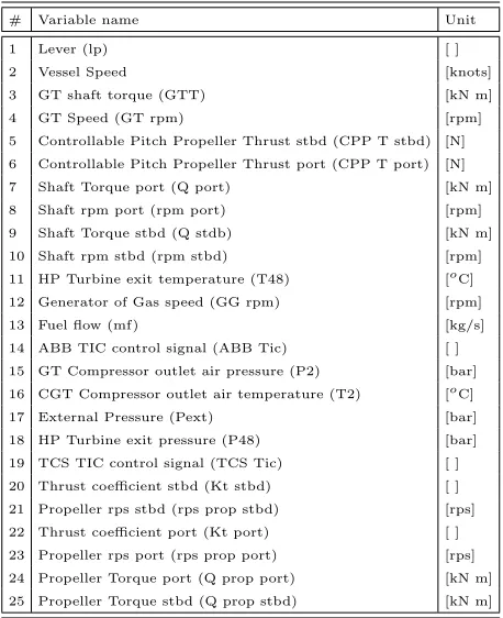
Once these quantities are fixed, the numerical model is run until the steady state is reached. Then, the model is able to provide all the quantities reported in Table 1. These subsets of models outputs are the same quantities that the automation system installed on-board can acquire and store.
The simulator was run on a server equipped with four Intel® Xeon® CPU E5-4620 2.2 GHz, 128 GB of RAM, 120 GB SSD disk, and Matlab® R2016a.
3.2. Condition-Based Maintenance
Table 1: Measured values available from the continuous monitoring system
# Variable name Unit
1 Lever (lp) [ ]
2 Vessel Speed [knots]
3 GT shaft torque (GTT) [kN m]
4 GT Speed (GT rpm) [rpm]
5 Controllable Pitch Propeller Thrust stbd (CPP T stbd) [N]
6 Controllable Pitch Propeller Thrust port (CPP T port) [N]
7 Shaft Torque port (Q port) [kN m]
8 Shaft rpm port (rpm port) [rpm]
9 Shaft Torque stbd (Q stdb) [kN m]
10 Shaft rpm stbd (rpm stbd) [rpm]
11 HP Turbine exit temperature (T48) [oC]
12 Generator of Gas speed (GG rpm) [rpm]
13 Fuel flow (mf) [kg/s]
14 ABB TIC control signal (ABB Tic) [ ]
15 GT Compressor outlet air pressure (P2) [bar]
16 CGT Compressor outlet air temperature (T2) [oC]
17 External Pressure (Pext) [bar]
18 HP Turbine exit pressure (P48) [bar]
19 TCS TIC control signal (TCS Tic) [ ]
20 Thrust coefficient stbd (Kt stbd) [ ]
21 Propeller rps stbd (rps prop stbd) [rps]
22 Thrust coefficient port (Kt port) [ ]
23 Propeller rps port (rps prop port) [rps]
24 Propeller Torque port (Q prop port) [kN m]
the data generated can be used to create effective predictive DDMs for the CBM of an NPS.
The data described in Section 3.1 contain two sets of information: one regarding the quantities that the automation system installed on-board can acquire and store and the other one regarding the associated state of decay (efficiency coefficient) of the different NPS components (GT, GTC, HLL, and PRP). This problem can be straightforwardly mapped into a classical multi-output regression problem (Vapnik, 1998; Coraddu et al., 2016) where the aim is to predict the actual decay coefficient based on the automation data coming from the sensors installed on-board.
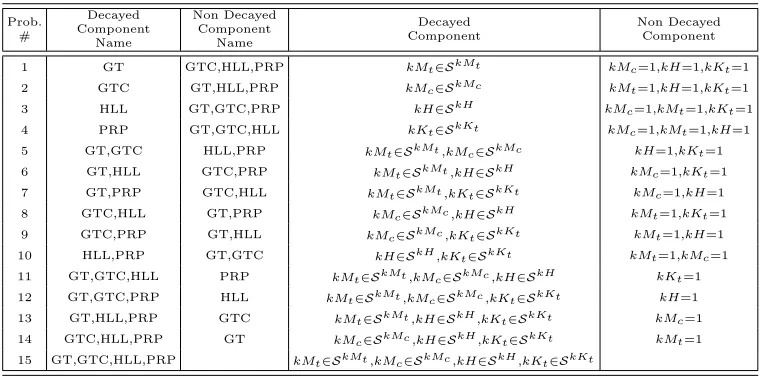
Since in authors’ analysis four different components of an NPS are taken into account (GT, GTC, HLL, and PRP), they decided to perform an incre-mental analysis by breaking down the problem into simpler ones. In partic-ular, first, only one NPS decayed component at the time is considered, then authors consider the possible combination of two NPS decayed components and so on until finally all the four NPS components are contemporarily con-sidered. Consequently, since four NPS components are considered, 4 = 41 problems have to be solved when just one NPS decayed component at the time is considered, then 6 = 42 problems have to be solved when two NPS decayed components at the time are considered and so on. Finally when all the four NPS components are contemporarily considered 1 = 44 problem has to be solved, for a total of 15 =P4
i=1 4
i
problems. Therefore, from the dataset described in Section 3.1, 15 sub-datasets corresponding to the cases mentioned above have been extracted. For the sake of clarity in Table 2 the 15 problems with the corresponding decay values are reported, not that in all the problems lp ∈ Slp.
4. Machine Learning Techniques
In this section, the authors will present the Machine Learning (ML) tech-niques adopted in order to build the CBM DDMs for NPS described in Sec-tion 2, based on the data outlined in SecSec-tion 3.
Let authors consider an input spaceX ⊆Rdand an output spaceY. Note
Table 2: The 15 sub-problems corresponding to considering different decayed component at the time
Prob. #
Decayed Component
Name
Non Decayed Component
Name
Decayed Component
Non Decayed Component
1 GT GTC,HLL,PRP kMt∈SkMt kMc=1,kH=1,kKt=1
2 GTC GT,HLL,PRP kMc∈SkMc kMt=1,kH=1,kKt=1
3 HLL GT,GTC,PRP kH∈SkH kM
c=1,kMt=1,kKt=1
4 PRP GT,GTC,HLL kKt∈SkKt kMc=1,kMt=1,kH=1
5 GT,GTC HLL,PRP kMt∈SkMt,kMc∈SkMc kH=1,kKt=1
6 GT,HLL GTC,PRP kMt∈SkMt,kH∈SkH kMc=1,kKt=1
7 GT,PRP GTC,HLL kMt∈SkMt,kKt∈SkKt kMc=1,kH=1
8 GTC,HLL GT,PRP kMc∈SkMc,kH∈SkH kMt=1,kKt=1
9 GTC,PRP GT,HLL kMc∈SkMc,kKt∈SkKt kMt=1,kH=1
10 HLL,PRP GT,GTC kH∈SkH,kK
t∈SkKt kMt=1,kMc=1
11 GT,GTC,HLL PRP kMt∈SkMt,kMc∈SkMc,kH∈SkH kKt=1
12 GT,GTC,PRP HLL kMt∈SkMt,kMc∈SkMc,kKt∈SkKt kH=1
13 GT,HLL,PRP GTC kMt∈SkMt,kH∈SkH,kKt∈SkKt kMc=1
14 GTC,HLL,PRP GT kMc∈SkMc,kH∈SkH,kK
t∈SkKt kMt=1
15 GT,GTC,HLL,PRP kMt∈SkMt,kMc∈SkMc,kH∈SkH,kKt∈SkKt
an elementy ∈ Y to an elementx∈ X. Note that, in general, µcan be non-deterministic. An ML technique estimates µ through a learning algorithm
AH:Dn×F → h, characterized by its set of hyperparametersH, which maps
a series of examples of the input/output relation contained in a datasets of
n samplesDn :{(x1, y1),· · · ,(xn, yn)} into a function f :X → Y chosen in
a set of possible ones F.
When both xi and yi with i ∈ {1,· · · , n} are available, the problems
is named supervised and consequently supervised ML technique are adopted (Vapnik, 1998). Regression is one of the most popular examples of supervised ML problems (Shawe-Taylor & Cristianini, 2004) which is characterized by
Y ∈ R.
The error thatf commits in approximating µis measured with reference to a loss function`:X ×Y ×F →[0,∞). Obviously, the error thatf commits over Dn, is optimistically biased since Dn has been used, together with F,
for building f itself. For this reason, another set of fresh data, composed of m samples and called test set Tm ={(xt1, yt1),· · · ,(xtm, ymt )}, needs to be
exploited. Note that, xt
i ∈ X and yit ∈ Y with i ∈ {1,· · · , m}, and the
association of yit to xti is again made based on µ. It has to be clarified that
Tm must contain both xti ∈ X and yit ∈ Y with i ∈ {1,· · · , m} to estimate
4.1. Measuring the Error
In this work, many state-of-the-art ML techniques will be tested and their performances will be compared to understand what is the most suited solution for building CBM DDMs for NPS.
In order to perform this analysis, authors have to define different measures of error, also called indexes of performance, able to well characterize the quality of the different CBM DDMs for NPS. Once f has been chosen based on Dn it is possible to use the fresh set of data Tm in order to compute its
error based on different losses. The choice of the loss strongly depends on the problem under examination (Rosasco et al., 2004).
In a typical regression framework, there are two losses that are mainly used for estimating the quality of a regressor: the absolute loss`1(f(x), y) = |f(x)−y|and the squared loss`2(f(x), y) = (f(x)−y)2. Based on these losses
it is possible to define different indexes of performance, which differently weight the distance between yt
i and f(xti) (Ghelardoni et al., 2013):
• the Mean Squared Error (MSE) is computed by taking the mean square loss value of f over Tm: MSE =1/mPmi=1`2(f(xti), yit);
• the Normalized Mean Square Error (NMSE) is similar to the MSE but a normalization term composed of the mean value of the differ-ence between the true values and their mean is applied: NMSE =
Pm
i=1`2(f(x
t i), y
t i)/∆;
• the Relative Error Percentage (REP) is similar to NMSE but the nor-malization term is composed of the sum of the squared true values. Then the result is square rooted and reported in percentage: REP = 100pPm
i=1`2(f(xti), yit)/Pmi=1(yt i)2;
• the Mean Absolute Error (MAE) is similar to MSE but the absolute loss is used instead: MAE = 1/mPm
i=1`1(f(xti), yit);
• the Mean Absolute Percentage Error (MAPE) can be described as the MAE expressed in percentage: MAPE =100/mPm
i=1`1(f(x
t
i), yit)/yti;
• the Pearson Product-Moment Correlation Coefficient (PPMCC) is a measure of the linear dependency between f(xti) and yti with i ∈ {1,
· · ·, m}: PPMCC = Pm
i=1(yti−y)(f(xit)−yˆ)/pPmi=1(yt i−y)2
pPn
i=1(f(xti)−yˆ)2,
where authors have exploited the following notation
y= 1
m
m
X
i=1
yit, ∆ = 1
m
m
X
i=1
(yit−y)2, yˆ= 1
m
m
X
i=1
4.2. Machine Learning Techniques
In this section, authors will present the supervised learning algorithms exploited in this paper for building CBM DDMs for NPS. Moreover, authors will show how to tune their performances by tuning their hyperparameters during the so-called Model Selection MS phase (Kohavi et al., 1995; Bartlett et al., 2002; Anguita et al., 2012). Finally, authors will also check for possi-ble spurious correlation in the data by performing the Feature Selection (FS) phase (Guyon & Elisseeff, 2003; Friedman et al., 2001; Yoon et al., 2005). In fact, once f is built based on the different learning algorithm and has been confirmed to be a sufficiently accurate representation of µ, it can be interesting to investigate how the model f is affected by the different fea-tures that have been exploited to build f itself during the feature ranking procedure (Guyon & Elisseeff, 2003). As authors will describe later, for some algorithms, the feature ranking procedure is a by-product of the learning process itself and allows to simply check the physical plausibility of f.
4.2.1. Supervised Regressive Learning Algorithms
Supervised ML techniques can be grouped into different families, accord-ing to the space of function F from which the learning algorithm chooses the particular f, the approximation of µ, based on the available data Dn.
In fact, techniques belonging to the same family, share an affine F. Among the several possible ML families, authors choose the state-of-the-art ones which are commonly adopted in real-world application, and, in each family, the best performing techniques are selected. In particular, Neural Networks (NNs), Kernel Methods (KMs), Ensemble Methods (EMs), Bayesian Meth-ods (BMs), and Lazy MethMeth-ods (LMs) are adopted.
NNs are ML techniques which combine together many simple models of a human brain neuron, called perceptrons (Rosenblatt, 1958), in order to build a complex network. The neurons are organized in stacked layers connected together by weights that are learned based on the available data via back-propagation (Rumelhart et al., 1988). The hyperparameters of an NN HNN
are the number of layersh1 and the number of neurons for each layerh2,iwith
i∈ {1,· · · , h1}. Note that it is assumed that NN with only one hidden layer
has h1 = 1. If the architecture of the NN consists of only one hidden layer,
while the ones of the output layers are computed according to the Regular-ized Least Squares (RLS) principle (Huang et al., 2015, 2006; Cambria & Huang, 2013). The hyperparameters of the ELM HELM are the number of
neurons of the hidden layer, h1, and the RLS regularization hyperparameter h2 (Huang et al., 2004).
KMs are a family of ML techniques which exploits the “Kernel trick” for distances in order to extend linear techniques to the solution of non-linear problems (Cristianini & Shawe-Taylor, 2000; Scholkopf, 2001). In the case of regression, KMs select f as the function which minimizes the tradeoff between the sum of the accuracy over the data, namely the empirical error, and the complexity of the solution, namely the regularization term (Rifkin et al., 2003; Cristianini & Shawe-Taylor, 2000). Two of the most known and effective KM techniques are Kernelized Regularized Least Squares (KRLS), and Support Vector Regression (SVR). The hyperparameters of the KRLS
HKRLS are: the kernel, which is usually fixed and in this paper author chose
the Gaussian Kernel for the reasons described in Keerthi & Lin (2003); Oneto et al. (2015), its hyperparameter h1 and the regularization hyperparameter h2. SVR, instead, is a method which roots in the Statistical Learning Theory
(Vapnik, 1998) and differs from the KRLS as it introduces an insensitivity value for the errors (Shawe-Taylor & Cristianini, 2004). The hyperparameters of the SVR HSVR are the same as the ones of KRLS plus the insensitivity
value h3.
EMs ML techniques relies on the simple fact that combining the output of several classifiers results in a much better performance than using any one of them alone (Germain et al., 2015; Breiman, 2001). Random Forest (RF) (Breiman, 2001) and Random Rotation Ensembles (RRF) (Blaser & Fryzlewicz, 2015), two popular state-of-the-art and widely adopted meth-ods, combine many decision trees in order to obtain a effective predictors which have limited hyperparameter sensitivity and high numerical robust-ness (Fern´andez-Delgado et al., 2014; Wainberg et al., 2016). Both RF and RRF have hidden hyperparameters which are considered fixed in this work because of their limited effect (Orlandi et al., 2016).
to the training data. The hyperparameter of the GP HGP is the parameter
which governs the Gaussians width h1.
LMs ML techniques are learning method in which the definition of f is delayed until f(x) needs to be computed (Duch, 2000). LMs approximate
µ locally with respect to x. K-Nearest Neighbors (KNN) is one of the most popular LM due to its implementation simplicity and effectiveness (Cover & Hart, 1967). The hyperparameter of the KNN HKNN is the number of
neighbors of x to be considered h1.
4.2.2. Model Selection
MS deals with the problem of tuning the hyperparameters of each learning algorithm (Anguita et al., 2012). Several methods exist for MS purpose: re-sampling methods, like the well-known k-Fold Cross Validation (KCV) (Ko-havi et al., 1995) or the nonparametric Bootstrap (BTS) approach (Efron & Tibshirani, 1994; Anguita et al., 2000) approaches, which represent the state-of-the-art MS approaches when targeting real-world applications. Re-sampling methods rely on a simple idea: the original datasetDnis resampled
once or many (nr) times, with or without replacement, to build two
inde-pendent datasets called training, and validation sets, respectivelyLr
l andVvr,
with r ∈ {1,· · · , nr}. Note that Lrl ∩ Vvr =, Lrl ∪ Vvr =Dn. Then, in order
to select the best combination the hyperparameters H in a set of possible
ones H={H1,H2,· · · } for the algorithm AH or, in other words, to perform
the MS phase, the following procedure has to be applied:
H∗ : min
H∈H
1
nr nr X
r=1
1
v X
(xi,yi)∈Vvr
`(AH,Lr
l(xi), yi), (14)
where AH,Lr
l is a model built with the algorithm A with its set of
hyper-parameters H and with the data Lr
l. Since the data in Lrl are independent
from the ones inVr
v, the idea is thatH
∗ should be the set of hyperparameters
which allows to achieve a small error on a data set that is independent from the training set.
If r = 1, if l and v are aprioristically set such that n =l+v, and if the resample procedure is performed without replacement, the hold out method is obtained (Anguita et al., 2012). For implementing the complete k-fold cross validation, instead, it is needed to setr≤ nk n−nk
k
,l= (k−2)nk,v = nk, and
the bootstrap, l = n and Lr
l must be sampled with replacement from Dn,
while Vr
v and Ttr are sampled without replacement from the sample of Dn
that have not been sampled in Lr
l (Efron & Tibshirani, 1994; Anguita et al.,
2012). Note that for the bootstrap procedure r ≤ 2n−n1
. In this paper the BTS is exploited because it represents the state-of-the-art approach (Efron & Tibshirani, 1994; Anguita et al., 2012).
4.3. Feature Selection
Once the CBM NPS models are built and have been confirmed to be sufficiently accurate representation of the real decays of the components, it can be interesting to investigate how these models are affected by the different features used in the model identification phase (see Table 1).
In DA this procedure is called FS or Feature Ranking (Guyon & Elisseeff, 2003; Friedman et al., 2001; Yoon et al., 2005). This process allows detecting if the importance of those features, that are known to be relevant from a physical perspective, is appropriately described by the different CBM NPS models. The failure of the statistical model to properly account for the relevant features might indicate poor quality in the measurements or spurious correlations. FS therefore represents an important step of model verification, since it should generate consistent results with the available knowledge of the physical system under exam.
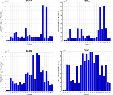
In addition, the EMs can also be used to perform a very stable FS proce-dure. The procedure is a combination of EMs, together with the permutation test (Good, 2013), in order to perform the selection and the ranking of the features. In details, for every tree, two quantities are computed: the first one is the error on the out-of-bag samples as they are used during prediction, while the second one is the error on the out-of-bag samples after a random permutation of the values of variablej. These two values are then subtracted and the average of the result over all the trees in the ensemble is the raw importance score for variable j (mean decrease in accuracy). This procedure was adopted since it can be easily carried out during the main prediction process inexpensively.
5. Experimental results
proposed regression framework, as described in Section 2, based on the data described in Section 3.
As described in Section 4, the authors tackle a regression problem where the actual value of the decay parameters needs to be estimated.
The different datasets considered in Section 3.2, corresponding to the 15 problems of Table 2 {P1,· · · , P15}, were divided into training and test set, respectively Dn and Tm, as reported in Section 4. Moreover, different
dimensions of the training set n∈ {10,24,55,130,307,722,1700,4000}were considered.
0 50 100 150 200 250 300 350 400
n 0 0.5 1 1.5 2 2.5 3 3.5 MAPE PRP KRLS ELM KNN RF GP SVR DNN RFR SNN
0 50 100 150 200 250 300 350 400
n 0 1 2 3 4 5 6 MAPE HLL KRLS ELM KNN RF GP SVR DNN RFR SNN
0 50 100 150 200 250 300 350 400
n 0 0.2 0.4 0.6 0.8 1 1.2 1.4 1.6 1.8 MAPE GTC KRLS ELM KNN RF GP SVR DNN RFR SNN
0 50 100 150 200 250 300 350 400
[image:18.612.124.486.270.572.2]n 0 0.1 0.2 0.3 0.4 0.5 0.6 0.7 0.8 MAPE GT KRLS ELM KNN RF GP SVR DNN RFR SNN
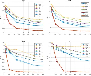
Figure 1: MAPE of the models learned with the different algorithms (DNN, SNN, ELM,
SVR, KRLS, KNN, and GP) when varyingnforP15 and for the four main NPS
compo-nents.
list of hyperparameters tested during the MS, with their respective intervals, is reported:
1. DNN: the set of hyperparameters is HDN N = {h
1, h2,1,· · · , h2,h1} and
authors chose it in HDNN={1,3,5,7,10} × {10,101.2· · · ,103} × · · · ×
{10,101.2· · · ,103};
2. SNN: the set of hyperparameters is HSN N ={h1} and authors chose it
in HSNN={1,3,5,7,10};
3. ELM: the set of hyperparameters is HELM = {h
1, h2} and authors
chose it in HELM ={10,101.2,· · · ,103} × {10−2,10−1.5· · · ,102}; 4. SVR: the set of hyperparameters is HSV R = {h
1, h2, h3} and authors
chose it in HSVR = {10−6,10−5,· · · ,103} × {10−2,10−1.4,· · · ,103} ×
{10−2,10−1.4 ,· · · ,103};
5. KRLS: the set of hyperparameters is HKRLS = {h
1, h2} and authors
chose it in HKRLS ={10−2,10−1.4,· · · ,103} × {10−2,10−1.4,· · · ,103};
6. KNN: the set of hyperparameters is HKN N = {h1} and authors chose
it in HKNN ={1,3,7,13,27,51};
7. GP: the set of hyperparameters isHGP ={h
1}and authors chose it in
HGP={100,100.3,· · · ,103};
The performances of each model are measured according to the metrics described in Section 4.1. Each experiment was performed 10 times in order to obtain statistical relevant result, and the t-student 95% confidence interval is reported when space in the table was available without compromising their readability.
For SNN and DNN the Python Keras library (Chollet, 2015) has been exploited. For ELM, SVR, KRLS, KNN, and GKNN a custom R implemen-tation has been developed. For RF the R package of Liaw & Wiener (2002) has been exploited. For RFE the implementation of Blaser & Fryzlewicz (2015) has been exploited. For GP the R package of Zeileis et al. (2004) has been exploited.
5.1. Regression Models Error Results
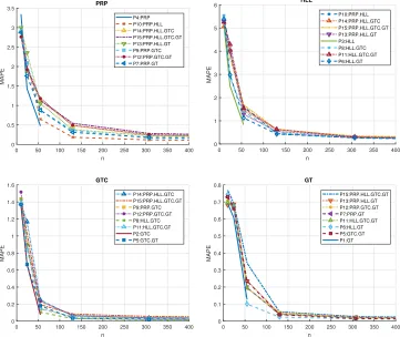
all the components decay contemporarily. In Figures 1 authors report the MAPE of the models learned with the different algorithms when varyingnfor
P15 and the four NPS components. In Figures 2 authors report the MAPE of the DNN (the best performing model) when varying n for the different problems under examination and the four NPS components.
0 50 100 150 200 250 300 350 400 n 0 0.5 1 1.5 2 2.5 3 3.5 MAPE PRP P4:PRP P10:PRP.HLL P14:PRP.HLL.GTC P15:PRP.HLL.GTC.GT P13:PRP.HLL.GT P9:PRP.GTC P12:PRP.GTC.GT P7:PRP.GT
0 50 100 150 200 250 300 350 400
n 0 1 2 3 4 5 6 MAPE HLL P10:PRP.HLL P14:PRP.HLL.GTC P15:PRP.HLL.GTC.GT P13:PRP.HLL.GT P3:HLL P8:HLL.GTC P11:HLL.GTC.GT P6:HLL.GT
0 50 100 150 200 250 300 350 400
n 0 0.2 0.4 0.6 0.8 1 1.2 1.4 1.6 MAPE GTC P14:PRP.HLL.GTC P15:PRP.HLL.GTC.GT P9:PRP.GTC P12:PRP.GTC.GT P8:HLL.GTC P11:HLL.GTC.GT P2:GTC P5:GTC.GT
[image:20.612.125.486.215.519.2]0 50 100 150 200 250 300 350 400 n 0 0.1 0.2 0.3 0.4 0.5 0.6 0.7 0.8 MAPE GT P15:PRP.HLL.GTC.GT P13:PRP.HLL.GT P12:PRP.GTC.GT P7:PRP.GT P11:HLL.GTC.GT P6:HLL.GT P5:GTC.GT P1:GT
Figure 2: MAPE of the models learned with DNN when varyingnfor the different problems
P1,· · ·, P15 and for the four main NPS components.
From the different figures it is possible to observe that:
• as expected the larger isn the better performances are achieved by the learned models (see Figures 2 and 1);
• the models learned with ELM, SNN, and especially DNN generally show the best performances (see Figure 1);
• the most complicate decay to predict is the one of the HLL, in fact the problems where the HLL decays are the ones which show lower accuracies (see Figure 2);
• unfortunately, as it can be seen from 2 and 1, this approach requires a significant amount of labelled data, which could not be retrieved in many operational scenarios. In fact, while the sensors data coming from the automation system are easy to collect, the information regarding the associated state of decay is not so easy to retrieve. Collecting the state of decay of the different NPS components requires the intervention of an experienced operator and, in some cases, to stop the vessel or even to put the ship in a dry dock.
1 2 3 4 5 6 7 8 910 11 12 13 14 15 16 17 18 19 20 21 22 23 24 25
feature 0 0.5 1 1.5 2 2.5 3 3.5 4 4.5
Mean Decrease in Accuracy
10-4 P1:PRP
1 2 3 4 5 6 7 8 910 11 12 13 14 15 16 17 18 19 20 21 22 23 24 25
feature 0 0.2 0.4 0.6 0.8 1 1.2 1.4 1.6 1.8
Mean Decrease in Accuracy
10-3 P2:HLL
1 2 3 4 5 6 7 8 910 11 12 13 14 15 16 17 18 19 20 21 22 23 24 25
feature 0 0.5 1 1.5 2 2.5 3 3.5 4 4.5 5
Mean Decrease in Accuracy
10-5 P3:GTC
1 2 3 4 5 6 7 8 910 11 12 13 14 15 16 17 18 19 20 21 22 23 24 25 feature 0 1 2 3 4 5 6 7 8 9
Mean Decrease in Accuracy
[image:21.612.124.490.299.606.2]10-6 P4:GT
Figure 3: FS performed with RF for the four main NPS components for problemP1,P2,
P3, andP4
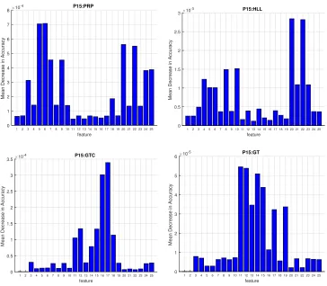
P1,P2,P3, and P4 (see Figure 3) and forP15 (see Figure 4). In particular, for each problem and each feature, the mean decrease in accuracy is reported as described in Section 4.3.
1 2 3 4 5 6 7 8 910 11 12 13 14 15 16 17 18 19 20 21 22 23 24 25 feature
0 1 2 3 4 5 6 7 8
Mean Decrease in Accuracy
10-4 P15:PRP
1 2 3 4 5 6 7 8 910 11 12 13 14 15 16 17 18 19 20 21 22 23 24 25
feature 0
0.5 1 1.5 2 2.5 3
Mean Decrease in Accuracy
10-3 P15:HLL
1 2 3 4 5 6 7 8 910 11 12 13 14 15 16 17 18 19 20 21 22 23 24 25 feature
0 0.5 1 1.5 2 2.5 3 3.5
Mean Decrease in Accuracy
10-4 P15:GTC
1 2 3 4 5 6 7 8 910 11 12 13 14 15 16 17 18 19 20 21 22 23 24 25
feature 0
1 2 3 4 5 6
Mean Decrease in Accuracy
[image:22.612.124.488.177.495.2]10-5 P15:GT
Figure 4: FS performed with RF for the four main NPS components for problemP15.
From Figure 3 and 4 it is possible to observe that:
• as expected, when just one component decays (see Figure 3), few pre-dictors have strong predictive power while when all the components decay (see Figure 4) many predictors need to be considered in order to achieve satisfying accuracies;
22 and 24 (Thrust coefficient stbd and port) have strong predictive power. Moreover, for the P3 (GTC decay) the features describing the thermodynamic process, 17,19, and 20 (GT Compressor outlet air pressure, External Pressure ,and HP Turbine exit pressure) have the highest predictive power. Finally, several features are necessary for the GT decay prediction in P4.
6. Conclusions
The behavior and interaction of the main components of Ship Propulsion Systems cannot be easily modeled with a priori physical knowledge, consid-ering the large amount of variables influencing them. In fact, in this work, authors showed that by exploiting the most recent statistical techniques and the large amount of historical data collected by the current on-board automa-tion systems it is possible to build effective Data-Driven Models which do not require any a priori knowledge. In particular, the developed models are able to continuously monitor the propulsion equipment to avoid Preventive or Corrective Maintenance and take decisions based on the actual condition of the propulsion plant. A naval ship, characterized by a COmbined Diesel ELectric And Gas propulsion plant, has been exploited to show the effective-ness of the proposed approaches. Because of confidentiality constraints with the Navy the authors used a real-data validated simulator and the dataset has been published for free use.
of the vessel. Vessels are rarely available in the harbour for maintenance, and the necessary parameters cannot be easily acquired when the ship is op-erative. Second, the experiments carried out are relative to a specific vessel, and this work cannot be straightforwardly mapped to any new ship without a further investigation on transfer learning to understand how to use available data from other vessels. To solve the first issue, the authors suggest the pos-sibility of adopting a relaxation on the decay value prediction requirement, by transforming the regression problem into a simpler one by predicting only the necessity of each component to be replaced or not, instead of the precise component decay. Moreover, in the future, authors will focus their efforts on the development of supervised and unsupervised methods which could solve this problem and allow a simplification of the data collection procedure.
References
Abu-Elanien, A. E. B., & Salama, M. M. A. (2010). Asset management techniques for transformers. Electric power systems research,80, 456–464.
Akinfiev, T. S., Armada, M. A., & Fernandez, R. (2008). Nondestructive testing of the state of a ship’s hull with an underwater robot. Russian Journal of Nondestructive Testing,44, 626–633.
Altosole, M., Benvenuto, G., & Campora, U. (2010). Numerical modelling of the engines governors of a codlag propulsion plant. In International Conference on Marine Sciences and Technologies.
Altosole, M., Benvenuto, G., Figari, M., & Campora, U. (2009). Real-time simulation of a cogag naval ship propulsion system.Journal of Engineering for the Maritime Environment,223, 47–62.
Altosole, M., Campora, U., Martelli, M., & Figari, M. (2014). Performance decay analysis of a marine gas turbine propulsion system. Journal of Ship Research, 58, 117–129.
Anguita, D., Boni, A., & Ridella, S. (2000). Evaluating the generalization ability of support vector machines through the bootstrap. Neural Process-ing Letters, 11, 51–58.
Anguita, D., Ghio, A., Greco, N., Oneto, L., & Ridella, S. (2010). Model selection for support vector machines: Advantages and disadvantages of the machine learning theory. InInternational Joint Conference on Neural Networks.
Anguita, D., Ghio, A., Oneto, L., & Ridella, S. (2012). In-sample and out-of-sample model selection and error estimation for support vector machines.
IEEE Transactions on Neural Networks and Learning Systems,23, 1390– 1406.
Arlot, S., & Celisse, A. (2010). A survey of cross-validation procedures for model selection. Statistics surveys, 4, 40–79.
Atlar, M., Glover, E. J., Candries, M., Mutton, R. J., & Anderson, C. D. (2002). The effect of a foul release coating on propeller performance. In
Marine Science and Technology for Environmental Sustainability.
Bache, K., & Lichman, M. (2013). UCI machine learning repository.
Bagavathiappan, S., Lahiri, B. B., Saravanan, T., Philip, J., & Jayakumar, T. (2013). Infrared thermography for condition monitoring-a review. Infrared Physics & Technology, 60, 35–55.
Bartlett, P. L., Boucheron, S., & Lugosi, G. (2002). Model selection and error estimation. Machine Learning, 48, 85–113.
Basurko, O. C., & Uriondo, Z. (2015). Condition-based maintenance for medium speed diesel engines used in vessels in operation. Applied Thermal Engineering, 80, 404–412.
Bengio, Y. (2009). Learning deep architectures for ai. Foundations and trends® in Machine Learning,2, 1–127.
Benvenuto, G., & Campora, U. (2007). Performance prediction of a faulty marine diesel engine under different governor settings. In International Conference on Marine Research And Transportation.
Bishop, C. M. (1995). Neural networks for pattern recognition. Oxford uni-versity press.
Blaser, R., & Fryzlewicz, P. (2015). Random rotation ensembles.The Journal of Machine Learning Research, 2, 1–15.
Boucheron, S., Bousquet, O., & Lugosi, G. (2005). Theory of classification: A survey of some recent advances. ESAIM: probability and statistics, 9, 323–375.
Breiman, L. (2001). Random forests. Machine learning, 45, 5–32.
Budai, G., Huisman, D., & Dekker, R. (2006). Scheduling preventive railway maintenance activities. The International Journal of Advanced Manufac-turing Technology, 57, 1035–1044.
Budai-Balke, G. (2009). Operations research models for scheduling railway infrastructure maintenance. Rozenberg Publishers.
Bunks, C., McCarthy, D., & Al-Ani, T. (2000). Condition-based maintenance of machines using hidden markov models. Mechanical Systems and Signal Processing, 14, 597–612.
Byington, C. S., Roemer, M. J., & Galie, T. (2002). Prognostic enhance-ments to diagnostic systems for improved condition-based maintenance. In Aerospace Conference.
Cambria, E., & Huang, G.-B. (2013). Extreme learning machines. IEEE Intelligent Systems, 28, 30–59.
Campora, U., & Figari, M. (2003). Numerical simulation of ship propul-sion transients and full-scale validation. Journal of Engineering for the Maritime Environment,217, 41–52.
Carlton, J. (2011). Marine propellers and propulsion. Butterworth-Heinemann.
Coraddu, A., Oneto, L., Baldi, F., & Anguita, D. (2015). Ship efficiency forecast based on sensors data collection: Improving numerical models through data analytics. In OCEANS 2015-Genova.
Coraddu, A., Oneto, L., Baldi, F., & Anguita, D. (2017). Vessels fuel con-sumption forecast and trim optimisation: A data analytics perspective.
Ocean Engineering, 130, 351–370.
Coraddu, A., Oneto, L., Ghio, A., Savio, S., Anguita, D., & Figari, M. (2016). Machine learning approaches for improving condition-based maintenance of naval propulsion plants. Proceedings of the Institution of Mechanical Engineers Part M: Journal of Engineering for the Maritime Environment,
230, 136–153.
Cover, T., & Hart, P. (1967). Nearest neighbor pattern classification. IEEE transactions on information theory, 13, 21–27.
Cristianini, N., & Shawe-Taylor, J. (2000). An introduction to support vector machines and other kernel-based learning methods. Cambridge university press.
Cybenko, G. (1989). Approximation by superpositions of a sigmoidal func-tion. Mathematics of Control, Signals, and Systems (MCSS),2, 303–314.
Danaos (2017). Planned maintenance system. https://danaosmc. wordpress.com/2016/03/30/planned-maintenance-system.
Das, S., & Chen, M. (2001). Yahoo! for amazon: Extracting market sen-timent from stock message boards. In Asia Pacific finance association annual conference (APFA).
DNV-GL (2017). Shipmanager technical. https://www.dnvgl.com/
services/planned-maintenance-system-for-technical-ship-management-shipmanager-technical-1509.
Duch, W. (2000). Similarity-based methods: a general framework for classi-fication, approximation and association. Control and Cybernetics,29.
Fern´andez-Delgado, M., Cernadas, E., Barro, S., & Amorim, D. (2014). Do we need hundreds of classifiers to solve real world classification problems.
The Journal of Machine Learning Research, 15, 3133–3181.
Figari, M., & Altosole, M. (2007). Dynamic behaviour and stability of marine propulsion systems.Journal of Engineering for the Maritime Environment,
221, 187–205.
Friedman, J., Hastie, T., & Tibshirani, R. (2001). The elements of statistical learning. Springer series in statistics Springer, Berlin.
Gelman, A., Carlin, J. B., Stern, H. S., & Rubin, D. B. (2014). Bayesian data analysis, vol. 2. Chapman and Hall/CRC.
Germain, P., Lacasse, A., Laviolette, F., Marchand, M., & Roy, J. F. (2015). Risk bounds for the majority vote: From a pac-bayesian analysis to a learning algorithm. The Journal of Machine Learning Research, 16, 787– 860.
Ghelardoni, L., Ghio, A., & Anguita, D. (2013). Energy load forecasting using empirical mode decomposition and support vector regression. IEEE Transactions on Smart Grid, 4, 549–556.
Good, P. (2013). Permutation tests: a practical guide to resampling methods for testing hypotheses. Springer Science & Business Media.
Guyon, I., & Elisseeff, A. (2003). An introduction to variable and feature selection. The Journal of Machine Learning Research,3, 1157–1182.
Gy¨orfi, L., Kohler, M., Krzyzak, A., & Walk, H. (2006). A distribution-free theory of nonparametric regression. Springer Science & Business Media.
Hadler, J. B., Wilson, C. J., & Beal, A. L. (1962). Ship standardisation trial performance and correlation with model predictions. In The Society of Naval Architects and Marine Engineers.
Hinton, G. E., Osindero, S., & Teh, Y. W. (2006). A fast learning algorithm for deep belief nets. Neural computation, 18, 1527–1554.
Huang, G.-B., Zhu, Q.-Y., & Siew, C.-K. (2004). Extreme learning machine: a new learning scheme of feedforward neural networks. In IEEE Interna-tional Joint Conference on Neural Networks.
Huang, G. B., Zhu, Q. Y., & Siew, C. K. (2006). Extreme learning machine: theory and applications. Neurocomputing, 70, 489–501.
ISO BS (2004). 13372: 2012, condition monitoring and diagnostics of machines-vocabulary. In British Standards.
Jackson, Y., Tabbagh, P., Gibson, P., & Seglie, E. (2005). The new depart-ment of defense (dod) guide for achieving and assessing ram. InReliability and Maintainability Symposium.
Jardine, A. K. S., Lin, D., & Banjevic, D. (2006). A review on machinery diagnostics and prognostics implementing condition-based maintenance.
Mechanical systems and signal processing,20, 1483–1510.
Keerthi, S. S., & Lin, C. J. (2003). Asymptotic behaviors of support vector machines with gaussian kernel. Neural computation, 15, 1667–1689.
Khor, Y. S., & Xiao, Q. (2011). Cfd simulations of the effects of fouling and antifouling. Ocean Engineering, 38, 1065–1079.
Kohavi, R. et al. (1995). A study of cross-validation and bootstrap for ac-curacy estimation and model selection. In International Joint Conference on Artificial Intelligence.
Kothamasu, R., & Huang, S. H. (2007). Adaptive mamdani fuzzy model for condition-based maintenance. Fuzzy Sets and Systems, 158, 2715–2733.
Lazakis, I., Dikis, K., Michala, A. L., & Theotokatos, G. (2016). Advanced ship systems condition monitoring for enhanced inspection, maintenance and decision making in ship operations. Transportation Research Procedia,
14, 1679–1688.
Liaw, A., & Wiener, M. (2002). Classification and regression by randomfor-est. R News,2, 18–22.
ocean-going ships: a review. Journal of Coatings Technology and Research,
12, 315–444.
Linoff, G. S., & Berry, M. J. A. (2011). Data mining techniques: for market-ing, sales, and customer relationship management. John Wiley & Sons.
Management, G. B. Q., Committee, S. S., & Institution, B. S. (1984). British Standard Glossary of Maintenance Management Terms in Terotechnology. British Standards Institution.
Mann, L., Saxena, A., & Knapp, G. M. (1995). Statistical-based or condition-based preventive maintenance? Journal of Quality in Maintenance Engi-neering, 1, 46–59.
Mannini, A., & Sabatini, A. M. (2010). Machine learning methods for classi-fying human physical activity from on-body accelerometers. Sensors, 10, 1154–1175.
Mathur, A., Cavanaugh, K. F., Pattipati, K. R., Willett, P. K., & Galie, T. R. (2001). Reasoning and modeling systems in diagnosis and prognosis. In SPIE Aerosense Conference.
Meher-Homji, C. B., Focke, A. B., & Wooldridge, M. B. (1989). Fouling of axial flow compressors - causes, effects, detection, and control. In Eigh-teenth Turbomachinery Symposium.
Michala, A. L., Lazakis, I., & Theotokatos, G. (2015). Predictive maintenance decision support system for enhanced energy efficiency of ship machinery. In International Conference on Shipping in Changing Climates.
Mobley, R. K. (2002). An introduction to predictive maintenance. Butterworth-Heinemann.
Nguyen, T. T. T., & Armitage, G. (2008). A survey of techniques for in-ternet traffic classification using machine learning. IEEE Communications Surveys & Tutorials,10, 56–76.
Oneto, L., Fumeo, E., Clerico, G., Canepa, R., Papa, F., Dambra, C., Mazz-ino, N., & Anguita, D. (2016b). Advanced analytics for train delay pre-diction systems by including exogenous weather data. In International Conference on Data Science and Advanced Analytics.
Oneto, L., Ghio, A., Ridella, S., & Anguita, D. (2015). Support vector machines and strictly positive definite kernel: The regularization hyper-parameter is more important than the kernel hyperhyper-parameters. In IEEE International Joint Conference on Neural Networks.
Orlandi, I., Oneto, L., & Anguita, D. (2016). Random forests model selection. InEuropean Symposium on Artificial Neural Networks, Computational In-telligence and Machine Learning.
Palm´e, T., Breuhaus, P., Assadi, M., Klein, A., & Kim, M. (2011). New alstom monitoring tools leveraging artificial neural network technologies. In Turbo Expo: Turbine Technical Conference and Exposition.
Pang, B., Lee, L., & Vaithyanathan, S. (2002). Thumbs up? sentiment classification using machine learning techniques. InACL-02 conference on Empirical methods in natural language processing-Volume 10.
Peng, Y., Dong, M., & Zuo, M. J. (2010). Current status of machine prognos-tics in condition-based maintenance: a review. The International Journal of Advanced Manufacturing Technology,50, 297–313.
Petersen, J. P., Winther, O., & Jacobsen, D. J. (2012). A machine-learning approach to predict main energy consumption under realistic operational conditions. Ship Technology Research, 59, 64–72.
Poyhonen, S., Jover, P., & Hyotyniemi, H. (2004). Signal processing of vi-brations for condition monitoring of an induction motor. In Symposium on Control, Communications and Signal Processing.
Rasmussen, C. E. (2006). Gaussian processes for machine learning. In Gaus-sian Processes for Machine Learning.
Rifkin, R., Yeo, G., & Poggio, T. (2003). Regularized least-squares classifica-tion. Nato Science Series Sub Series III Computer and Systems Sciences,
Rosasco, L., De Vito, E., Caponnetto, A., Piana, M., & Verri, A. (2004). Are loss functions all the same? Neural Computation, 16, 1063–1076.
Rosenblatt, F. (1958). The perceptron: a probabilistic model for information storage and organization in the brain. Psychological review,65, 386.
Rumelhart, D. E., Hinton, G. E., & Williams, R. J. (1988). Learning repre-sentations by back-propagating errors. Cognitive modeling, 5, 1.
Scholkopf, B. (2001). The kernel trick for distances. In Advances in neural information processing systems.
Shawe-Taylor, J., & Cristianini, N. (2004). Kernel methods for pattern anal-ysis. Cambridge university press.
Shin, K., Lee, T. S., & Kim, H. (2005). An application of support vector ma-chines in bankruptcy prediction model. Expert Systems with Applications,
28, 127–135.
Simani, S., Fantuzzi, C., & Patton, R. J. (2003). Model-based Fault Diagno-sis in Dynamic Systems Using Identification Techniques. Springer-Verlag London.
Singer, R. M., Gross, K. C., & King, R. W. (1995). A pattern-recognition-based, fault-tolerant monitoring and diagnostic technique. In Argonne National Lab., Idaho Falls, ID (United States).
Smith, T. W. P., O’Keeffe, E., Aldous, L., & Agnolucci, P. (2013). As-sessment of shipping’s efficiency using satellite ais data. In International Council on Clean Transportation.
Spectec (2017). Amos maintenance-materials-management. http://www. spectec.net/maintenance-materials-management.
Tarabrin, A. P., Schurovsky, V. A., Bodrov, A. I., & Stalder, J. P. (1998). An analysis of axial compressor fouling and a blade cleaning method. Journal of Turbomachinery, 120, 256–261.
Waeyenbergh, G., & Pintelon, L. (2002). A framework for maintenance con-cept development.International journal of production economics,77, 299– 313.
Wainberg, M., Alipanahi, B., & Frey, B. J. (2016). Are random forests truly the best classifiers? The Journal of Machine Learning Research, 17, 1–5.
Wan, B., Nishikswa, E., & Uchida, M. (2002). The experiment and numerical calculation of propeller performance with surface roughness effects.Journal of the Kansai Society of Naval Architects, Japan, 2002, 49–54.
Wang, H., Osen, O. L., Li, G., Li, W., Dai, H., & Zeng, W. (2015). Big data and industrial internet of things for the maritime industry in northwestern norway. In IEEE Region 10 Conference TENCON.
Widodo, A., & Yang, B. (2007). Support vector machine in machine condition monitoring and fault diagnosis. Mechanical systems and signal processing,
21, 2560–2574.
Witten, I. H., Frank, E., Hall, M. A., & Pal, C. J. (2016). Data Mining: Practical machine learning tools and techniques. Morgan Kaufmann.
Yoon, H., Yang, K., & Shahabi, C. (2005). Feature subset selection and fea-ture ranking for multivariate time series. IEEE transactions on knowledge and data engineering,17, 1186–1198.