Supermetric search

Supermetric Search

Richard Connora,∗, Lucia Vadicamob, Franco Alberto Cardilloc, Fausto Rabittib

a_{Department of Computer and Information Sciences, University of Strathclyde, Glasgow,} United Kingdom

b_{Institute of Information Science and Technologies (ISTI), CNR, Pisa, Italy} c_{Institute of Computational Linguistics (ILC), CNR, Pisa, Italy}

Abstract

Metric search is concerned with the efficient evaluation of queries in metric spaces. In general, a large space of objects is arranged in such a way that, when a further object is presented as a query, those objects most similar to the query can be efficiently found. Most mechanisms rely upon the triangle inequality property of the metric governing the space. The triangle inequality property is equivalent to a finite embedding property, which states that any three points of the space can be isometrically embedded in two-dimensional Euclidean space. In this paper, we examine a class of semimetric space which is finitely four-embeddable in three-dimensional Euclidean space. In mathematics this property has been extensively studied and is generally known as thefour-point property. All spaces with the four-point property are metric spaces, but they also have some stronger geometric guarantees. We coin the term supermetric1 _{space as,} in terms of metric search, they are significantly more tractable. Supermetric spaces include all those governed by Euclidean, Cosine2_{, Jensen-Shannon and} Triangular distances, and are thus commonly used within many domains. In previous work we have given a generic mathematical basis for the supermetric property and shown how it can improve indexing performance for a given exact search structure. Here we present a full investigation into its use within a variety of different hyperplane partition indexing structures, and go on to show some more of its flexibility by examining a search structure whose partition and exclusion conditions are tailored, at each node, to suit the individual reference points and data set present there. Among the results given, we show a new best performance for exact search using a well-known benchmark.

∗_{Corresponding author}

Email addresses: [email protected](Richard Connor),

[email protected](Lucia Vadicamo),[email protected]

(Franco Alberto Cardillo),[email protected](Fausto Rabitti)

1_{This term has previously been used in the domains of particle physics and evolutionary}

biology as a pseudonym for the mathematical termultra-metric, a concept of no interest in metric search; we believe our concept is of sufficient importance to the domain to justify its reuse with a different meaning.

Keywords: Similarity Search, Metric Space, Supermetric Space, Metric Indexing, Four-point Property, Hilbert Exclusion

1. Introduction

Within any metric space, any three objects can be used to construct a trian-gle in 2D Euclidean space, where the objects are represented by the vertices of the triangle and the edges preserve their distances in the original space. That is, any metric space is isometrically three-embeddable in 2D Euclidean space.

Some metric spaces are also isometrically four-embeddable in 3D Euclidean space, allowing the construction of a tetrahedron. We have previously shown how these spaces have further geometric properties which can be used to improve the performance of exact search, in particular for any search mechanism based on hyperplane partitioning. This leads to the notion of a supermetric space

[2], a space which is also a metric space but with further geometric properties which give stronger guarantees for search mechanisms. Furthermore, we have given a rigorous and constructive mathematical basis for assessing whether a proper metric space has the supermetric property, and showed how this property allows the use of the Hilbert Exclusion mechanism in place of the less powerful hyperbolic exclusion [1]. In [2], we also showed how the supermetric property could, in principle, be used to construct arbitrary partitions within a 2D plane into which many objects are projected, due to a lower-bound property which is a corollary of the four-point property.

In this paper we extend initial work which appeared in [2] by taking the investigation to its next stage. While we previously showed how the use of the Hilbert Exclusion property gave a significant improvement in performance when used in conjunction with a particular state-of-the-art hyperplane-based indexing mechanism, the Distal Spatial Approximation Tree (DiSAT, [3]), we now perform a full evaluation over its performance within a fully general context of twelve different hyperplane tree indexing structures. The outcome is that a simpler data structure is found to be the most efficient in this context, and indeed gives a new best-published performance for threshold search over the SISAP benchmark data sets [4]; to put this result in perspective, it requires only around 40% of the number of distance calculations per query of the previous state of the art given in [3].

Beyond these benchmark data sets, which in this context are relatively small and tractable, we show the performance advantages hold in some larger data sets, as dimensionality and object size increase, and also for a number of different distance metrics.

manifests differently with each choice of reference points, and this data structure allows a different strategy to be used in each node, to maximise the advantage which can be gained.

The rest of this paper is organised as follows. Section 2 sets the detailed technical context for the work, including related work by ourselves and others. Section 3 then explains a novel observation which is a consequence of the four-point property: tetrahedral projection onto a plane, which gives an important lower-bound property. In fact, it turns out that Hilbert Exclusion results as a simple corollary of this more general property. In this section we discuss a number of relatively deep results which are consequent to the property. Section 4 then fully defines a completely novel indexing structure which is only possible to use in a supermetric space, where the hyperplane partition and consequent exclusion mechanism are dynamically chosen according to the distribution of data within each individual node of the tree.

Section 5 takes as its starting point the observation that the best indexing techniques are likely to be different in the supermetric context, and gives a full investigation of various hyperplane trees in order to determine the most suit-able. Section 6 analyses the extra cost required to make use of the supermetric properties for hyperplane indexing, which in fact is very small. Section 7 exam-ines the use of the best data structures identified through their application to a number of large and real-world data sets, in order to test their performance in more general contexts.

Finally in Section 8 we give some conclusions and outline areas of further work.

2. Preliminaries and Related Work

To set the context, we are interested in searching a (large) finite set of objects Swhich is a subset of an infinite setU, where (U, d) is ametric space. A metric space is an ordered pair (U, d), where U is a domain of objects and d is a total distance functiond:U ×U →_R, satisfying postulates of non-negativity, identity, symmetry, and triangle inequality [5]. The general requirement is to efficiently find members of S which are similar to an arbitrary member of U, where the distance function d gives the only way by which any two objects may be compared - the bigger the distance d(x, y), the less similar the data objects x, y ∈ U. There are many important practical examples captured by this mathematical framework, see for example [6, 5]. Such spaces are typically searched with reference to a query objectq∈U. The simplest type of similarity query is therange search query. A range search for some thresholdt, based on a queryq ∈ U, has the solution set R = {s ∈S|d(q, s) ≤t}. Other forms of search, for example nearest neighbor search (i.e. find the k closest objects to a query), are also useful; here we are studying mostly properties of spaces in general and restrict our attention to the scenario outlined.

Notion Definition

(U, d) the data domainU and the metric distanced:U×U→R

S finite set of data objects,S⊆U

x, y, s generic data object,x, y, s∈S

q query objectq∈U

t, ti threshold distances used in the range search,t, ti∈R

R solution set for a range query: R={s∈S|d(q, s)≤t}

{p1, . . . , pn} set ofnpivots,pi∈U

`2 Euclideandistance: `2(x, y) =pPn

i=1(xi−yi)2 forx, y∈Rn `n

2 n-dimensional Euclideanspace,i.e. (Rn, `2).

For example,`n

2 = (Rn, `2),`32= (R3, `2)

Isometric 3-embedding in`2

2

A metric space (U, d) is isometrically 3-embeddable in `2

2 if for any

three pointsx1, x2, x3 ∈U there exists a functionf :U →`22 such

that`2(f(xi), f(xj)) =d(xi, xj), fori, j= 1,2,3

Isometric 4-embedding in`3

2

A metric space (U, d) is isometrically 4-embeddable in `3

2 if for any

four pointsx1, x2, x3, x4∈U there exists a functionf:U→`22 such

that`2(f(xi), f(xj)) =d(xi, xj), fori, j= 1,2,3,4

four-point property

A metric space (U, d) has the four-point property if it is isometrically

4-embeddable in`32

vw line between two pointsv, w∈Rn

Table 1: Notation used throughout this paper

2.1. Metric indexing

Typically, the distance function is too expensive orS is too large to allow an exhaustive search, that is a sequential scan of the entire dataset. The retrieval process is facilitated by using a metric index, one of a large family of data structures used to preprocess the data in such a way as to minimise the time required to retrieve the query result. This data structure can be expensive to build, but this cost is amortized by saving I/O and distance evaluations over several queries to the database. In general, the triangle inequality property is exploited to determine subsets of S which do not need to be exhaustively checked. Such avoidance is normally referred to asexclusion orspace pruning.

For exact metric search, almost all indexing methods can be divided into those which at each exclusion possibility use a single “pivot” point to give radius-based exclusion, and those which use two reference points to give hyperplane-based exclusion. Many variants of each have been proposed, including many hybrids; [5], [7], and [8] give excellent surveys. In general the best choice seems to depend on the particular context of metric and data.

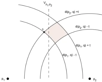
Figure 1: In any metric space, two pivot pointsp1, p2 and any solution to a queryqcan be isometrically embedded in`2

2. The point q cannot be drawn in the same diagram. Given its distance fromp1 andp2, any solution in the original metric space must lie in the region bounded by the four arcs shown. If the pointslies to the right ofVp1,p2 ={x∈S|d(x, p1) = d(x, p2)}, there is therefore no requirement to search to the left of the hyperplane in the original space. In general, when relying only on the triangle inequality, then half of the space can be excluded from the search only if|d(q, p1)−d(q, p2)|>2t.

Monotonous Bisector Trees [11] and Voronoi Trees [12]), the Metric Index [13], and the Spatial Approximation Tree [14]. This last has various derivatives, notably including the Dynamic SAT [15] and the Distal SAT (DiSAT) [3].

2.2. Metric Spaces and Finite Isometric Embeddings

An isometric embedding of one metric space (V, dv) in another (W, dw) can be

achieved when there exists a mapping functionf :V →W such thatdv(x, y) =

dw(f(x), f(y)), for all x, y∈V. A finite isometric embedding occurs whenever

this property is true for any finite selection ofn points fromV, in which case the terminology used is thatV is isometricallyn-embeddable inW.

The idea of characterising a space metrically by means of “n-point rela-tions” seems to have originated in the paper [16] published in 1892 by de Tilly, a Belgian artillery officer. Some of the questions raised by de Tilly were an-swered by some mathematicians of the late 19th century, and only in 1928 Karl Menger [17] provided a first systematic development of abstractdistance geom-etry. The interest of the distance geometry is in all those of transformations of sets for which the distance of two points is an invariant. So, as highlighted by Blumenthal [18], “distance geometry may operate in any kind of space in which a notion of “distance” is attached to any point-pair of the space”.

Isometric 3-embedding in `2

2. The first observation to be made in this context is that any metric space (U, d) is isometrically 3-embeddable in `2

2, i.e. for any three pointsx1, x2, x3∈U there exists a mapping functionf : (U, d)→(R2, `2) such that`2(f(xi), f(xj)) =d(xi, xj), for i, j = 1,2,3. This is apparent from

in `2<sub>2</sub>, triangle inequality also holds. It is interesting to consider the standard exclusion mechanisms of pivot-based exclusion and hyperplane-based exclusion in the light of an isometric 3-embedding in`22; Figure 1 for example shows a basis for hyperplane exclusion using only this property rather than triangle inequality explicitly.

Supermetric Spaces: Isometric 4-embedding in`3

2. It turns out that many useful metric spaces have a stronger property: they are isometrically 4-embeddable in

`3<sub>2</sub>, which means that for any four points in the space there exists an embedding into (R3, `2) that preserves all the 4₂

= 6 interpoint distances. In the math-ematical literature, this has been referred to as the four-point property [18]. Wilson [19] shows various properties of such spaces, and Blumenthal [18] points out that results given by Wilson, when combined with work by Menger [17], generalise to show that some spaces have then-point property: that is, anyn points can be isometrically embedded in a Euclidean (n−1)-dimensional space. We have studied such spaces in the context of metric indexing in [1], where we develop in detail the following outcomes:

1. Any metric space which is isometrically embeddable in a Hilbert space3 has then-point property, and so thefour-point property as well.

2. Important spaces with the n-point property include, for any dimension, spaces with the following metrics: Euclidean, Jensen-Shannon, Triangular, and (a variant of) Cosine distances.

3. Important spaces which do not have thefour-point property include those with the metrics: Manhattan, Chebyshev, and Levenshtein distances. 4. However, for any metric space (U, d), the space (U, dα), 0 < α≤ 1

2 does have thefour-point property.

In terms of practical impact on metric search, in [1] we show only how the four-point property can be used to improve standard hyperplane partitioning. We consider a situation where a subspace is divided according to which of two selected reference pointsp1andp2 is the closer. When relying only on triangle inequality, that is in a metric space without the four-point property, then for a queryqand a query thresholdt, the subspace associated withp1can be excluded from the search only ifd(q, p1)−d(q, p2) >2t. As the region defined by this condition when projected onto the plane is a hyperbola (see Figure 1), we name thisHyperbolic Exclusion4.

If the space in question has thefour-point property, however, we show that, for the same subspaces, there is no requirement to search that associated with

3_{A Hilbert spaceH can be thought of as a generalization of Euclidean space to any finite}

or infinite number of dimensions. It is an inner vector space which is also a complete metric space with respect to the distance function induced by the inner product. This means that it has an inner product<·,·>:H×H→_Cthat induces a distanced(·,·) =√<·,·>such that every Cauchy sequence in (H, d) converges to a point inH (intuitively, there are no “points missing” fromH).

4_{In the literature, the Hyperbolic Exclusion is also referred to asDouble-Pivot Distance}

p1 whenever

d(q, p1)2−d(q, p2)2 d(p1, p2)

>2t;

this is a weaker condition and therefore allows, in general, more exclusion. We name this conditionHilbert Exclusion.

A formula equivalent to

|d(q, p1)2−d(q, p2)2| 2d(p1, p2)

has been used in the context of metric search also in [20, 21], in order toestimate

the distance between the pointq and the hyperplane equidistant from p1 and p2. This formula was derived using the cosine law and was applied only with distances on metric space with the “semidefinite positive property” [20, 22], since this property allows defining a notion of “angle” in a generic metric space. To provide a bridge to our work, we observe that the semidefinite positive property is equivalent to then-point property for a finite semimetric space (see Chapter IV, Section 43 of [18]).

In this paper, we examine a more general consequence of four-point em-beddable spaces and show some interim results including new best-performance search of SISAP data sets.

3. Tetrahedral Projection onto a Plane

In a supermetric space, any two reference pointsp1andp2, and query point q,andany solution to that queryswhered(q, s)≤t, canallbe embedded in 3D Euclidean space. As such, they can be used to form the vertices of a tetrahedron. It seems that, while simple metric search is based around the properties of a triangle, there should be corresponding tetrahedral properties which give a new, stronger, set of guarantees.

Assume that for some search context, pointsp1, p2∈Uare somehow selected and a data structure is built for a finite setS ⊂U where, fors∈S, the three distancesd(p1, p2), d(s, p1) andd(s, p2) are calculated during the build process and used to guide the structuring of the data. At query time, for a query q, the two distancesd(q, p1) andd(q, p2) are calculated and may be used to make some deduction relating to this structure.

This situation gives knowledge of two adjacent faces of the tetrahedron which can be formed in three dimensions. Five of the six edge lengths have been measured, and the final edge is upper-bounded by the value oft. Therefore, for a pointsto be a solution to the query, it must be possible to form a tetrahedron with the five measured edge lengths, and a last edge of lengtht.

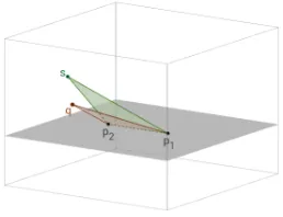
Figure 2: Two triangles with a common base in 3D space

Figure 3: Projection of the two triangles onto the same plane by rotation aroundp1p2. Note that`22(R(q), s)≤`32(q, s), where R(q) is the point obtained by rotatingqaround the line p1p2until it is coplanar withs

be achieved by rotating one of them around the linep1p2 until it is coplanar with the other, then for any case where the final edge of the tetrahedron (qs) is less than the length t, then the length of this side in the resulting planar tetrahedron is upper bounded byt, as illustrated in Figure 3.

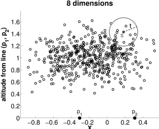
Many such coplanar triangles can be depicted, representing many points in a single space, in a single scatter plot as in Figure 4. This shows a set of 500 points, drawn from randomly generated 8-dimensional Euclidean space, and plotted with respect to their distances from two fixed reference pointsp1andp2. The distance between the reference points is measured, and the reference points are plotted on the X-axis symmetrically either side of the origin. For each point in the rest of the set, the distancesd(s, p1) andd(s, p2) are calculated, and used to plot the unique corresponding point in a triangle above the X-axis, according to these edge lengths. In this figure, in consideration with our observations over Figure 3, it can be seen that, if any two points are separated by less that some constantt in the original space, and thus also in the 3D embedding, then they are also withintof each other in this scatter plot.

Figure 4: Scatter diagram for 8-dimensional Euclidean Space. The distanceδ between two selected reference pointsp1andp2is measured, and an embedding function is chosen which maps these to (0,−δ/2) and (0, δ/2) respectively. Other pointssi in the space are then

plotted to preserve the distancesd(si, p1) andd(si, p2). For metric spaces with the four-point property, the`2distance between the corresponding points in this diagram is a lower bound ond(si, sj) in the original space. Hence, any point withintof a pointsin the original space

cannot lie outside the circle of radiustcentered aroundsin the scatter plot.

a simple metric space, but in this case no spatial relationship is implied between any two points plotted: no matter how close two points are in the plot, there is no implication for the distance between them in the original space. However if the diagram is plotted for a metric with the four-point property, then the distance between any two points on the plane is a lower bound on their distance in the original space; two points that are further than t on the plot cannot be within t of each other in the original space. This observation leads to an arbitrarily large number of ways of partitioning the space and allowing these partitions to excluded based on a query position, and has many potential uses in metric indexing.

3.1. Indexes Based on Tetrahedral/Planar Projection

During construction of an index, the constructed 2D space can be arbitrarily partitioned according to any rule based on the geometry of this plane, calculated with respect to the distances d(si, p1), d(si, p2) and d(p1, p2). At query time, if the query falls in any region of the plane that is further than the query thresholdtfrom any such partition, points within that partition cannot contain any solution to the query. Since, as will be shown, different spaces give quite different distributions of points within the plane, build-time partitions can be chosen according to this distribution, rather than as a fixed attribute of an index mechanism.

−0.8 −0.6 −0.4 −0.2 0 0.2 0.4 0 0.2 0.4 0.6 0.8 1 1.2 1.4 1.6 p

1 p2

Hilbert Exclusion, 8 dimensions

X

altitude from line (p

1

, p

2

)

non−exclusive queries exclusive queries, n = 340

−0.8 −0.6 −0.4 −0.2 0 0.2 0.4

0 0.2 0.4 0.6 0.8 1 1.2 1.4 1.6 p

1 p2

Hyperbolic Exclusion, 8 dimensions

X

altitude from line (p

1

, p

2

)

non−exclusive queries exclusive queries, n = 79

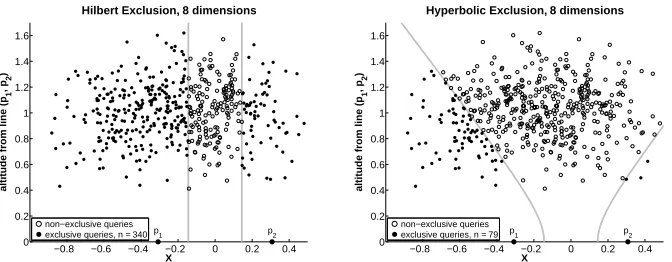
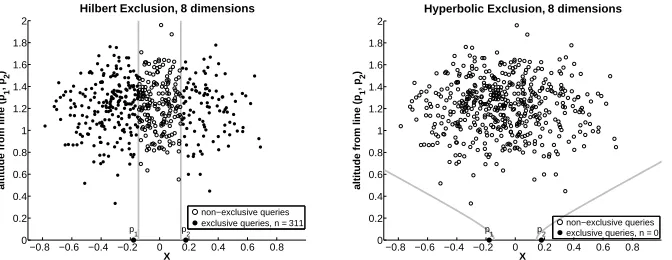
Figure 5: Scatter diagram for 8-dimensional Euclidean Space. The data is divided into two subsets according to which side of Y-axis they lie. The solidly-coloured points are points that, were they queries, would allow the semispace on the opposing side to be excluded from the search since that semispace cannot contain a solution. We refer to these points as “exclusive queries”. The other points are referred to as “non-exclusive queries” since they do not allow the opposing semispace to be excluded from the search. The left-hand side illustrates use of tetrahedral/planar projection, the right hand side illustrates use of the normal hyperbolic condition.

time, if the corresponding plot position for the query is further than t from the Y axis, no solutions can exist in the subset closer to the opposing reference point. Figure 5 shows the same points, but now highlighted according to this distinction. Those drawn in solid, either side of the Y-axis, are guaranteed to be on the same side of the corresponding hyperplane partition in the original space; therefore, if they were query points, the opposing semi-space would not require to be searched. We refer to these points as “exclusive queries”. If the same diagram is drawn for a simple metric space, a query point can be used to exclude the opposing semi-space only according to a condition algebraically derived from triangle inequality: |d(q, p1)−d(q, p2)| > 2t, which describes a hyperbola with foci at the reference points and semi-major axis of the search threshold. For the same data and search threshold, the difference in exclusion capability is shown in Figure 5; of the 500 randomly selected queries, only 160 fail to exclude the opposing semi-space, whereas with normal hyperbolic exclusion, the number is 421. The query threshold illustrated, 0.145, is chosen to retrieve around one millionth of the space and is not therefore artificially large.

As stated, this particular situation has been extensively investigated and is fully reported in [1]. Here we will concentrate further on other properties of the planar projection, of which the derivation of Hilbert exclusion turns out to be a special case.

3.2. Partitions of the 2D Plane

−0.8 −0.6 −0.4 −0.2 0 0.2 0.4 0.6 0.8 0

0.2 0.4 0.6 0.8 1 1.2

Hilbert Exclusion, 8 dimensions

X

altitude from line (p

1

, p

2

)

non−exclusive queries exclusive queries, n = 330

−0.8 −0.6 −0.4 −0.2 0 0.2 0.4 0.6 0.8

0 0.2 0.4 0.6 0.8 1 1.2

Hyperbolic Exclusion, 8 dimensions

X

altitude from line (p

1

, p

2

)

non−exclusive queries exclusive queries, n = 278

Figure 6: Scatter diagram for 8-dimensional Euclidean Space with widely separated reference points. (The distance between reference points is such that the reference points themselves do not appear on the plot).

all cases by implication there exists a simple binary partition tree structure corresponding to the partitioning. In all cases the partition is defined in terms of the 2D plane onto which all points are projected as described above.

3.3. Reference Point Separation

An important observation is that the shape of the 2D “point cloud”, upon which effective exclusion depends, is not greatly affected by the choice of ref-erence points. In comparison with normal Hyperbolic exclusion this is a huge advantage. The hyperbola which bounds the effective queries, i.e. those which can be used to exclude the opposing semispace, is defined only by the (fixed) query radius, and the distance between the reference points, where the larger the separation of the reference points, the better the exclusion. In the extreme case where the separation is no larger than twice the query radius, which can readily occur in high-dimensional space, it is impossible for any exclusions to be made. This effect can be ameliorated by choosing widely separated reference points, but in an unevenly distributed set this in itself can be dangerous: if one point chosen is an outlier, then the point cloud will lie close to the other point, and again no exclusions will be made. Finding two reference points which are well separated, and where the rest of the points is evenly distributed between them, is of course an intractable task in general.

−0.8 −0.6 −0.4 −0.2 0 0.2 0.4 0.6 0.8 0 0.2 0.4 0.6 0.8 1 1.2 1.4 1.6 1.8 2

p₁ p₂ Hilbert Exclusion, 8 dimensions

X

altitude from line (p

1

, p

2

)

non−exclusive queries exclusive queries, n = 311

−0.8 −0.6 −0.4 −0.2 0 0.2 0.4 0.6 0.8 0 0.2 0.4 0.6 0.8 1 1.2 1.4 1.6 1.8 2

p₁ p₂

Hyperbolic Exclusion, 8 dimensions

X

altitude from line (p

1

, p

2

)

non−exclusive queries exclusive queries, n = 0

Figure 7: Scatter diagram for 8-dimensional Euclidean Space with close reference points. Note from comparison of the left-hand graphs of this figure with Figure 6 that the separation of the reference points has no apparent effect on the power of the four-point exclusion, whereas normal metric exclusion becomes completely useless.

From Figure 6 it should also be noted that, no matter how far the reference points are separated, the four-point property always gives a higher probability of exclusions; in this case, although the separating lines do not appear visually to be very different, the implied probability of exclusion in for the four-point property is 0.66, against 0.56.

To allow most partition structures to perform well, a very large part of the build cost is typically spent in the selection of good reference points and this cost is largely avoidable with any such four-point strategy, as demonstrated experimentally in Sections 5 and 4.

3.4. Arbitrary Partitions

Again we stress the fact that, given the strong lower bound condition on the projected 2D plane, we can choose arbitrary geometric partitions of this plane to structure the data. For randomly generated, evenly distributed points there seems to be little to choose. However it is often the case that “real world” data sets do not show the same properties as generated sets; in particular, they tend to be much less evenly distributed, with significant numbers of clusters and outliers. These factors can significantly affect the performance of indexing mechanisms.

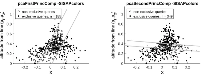
Figures 8, 9, 10 and 11 show a sample taken from the SISAP colors data set with Euclidean distance applied, showing eight different partitions. Eight different partitions of the plane have been arbitrarily selected and applied. The query threshold illustrated is 0.052 corresponding to a query returning 0.001% of the data.

-0.2 -0.1 0 0.1 0.2 X 0 0.2 0.4 0.6 0.8 1

altitude from line (p

1

,p2

)

vertical -SISAP colors

p₁ p₂

non-exclusive queries exclusive queries, n = 195

-0.2 -0.1 0 0.1 0.2 X 0 0.2 0.4 0.6 0.8 1

altitude from line (p

1

,p2

)

horizontal -SISAP colors

p₁ p₂

non-exclusive queries exclusive queries, n = 342

Figure 8: Scatter diagrams dividing the plane equally in X and Y dimension, either can be used for partitioning a hyperplane tree structure; in this case, the horizontal partition would be more effective.

-0.2 -0.1 0 0.1 0.2 X 0 0.2 0.4 0.6 0.8 1

altitude from line (p

1

,p2

)

pcaFirstPrincComp -SISAP colors

p₁ p₂

non-exclusive queries exclusive queries, n = 185

-0.2 -0.1 0 0.1 0.2 X 0 0.2 0.4 0.6 0.8 1

altitude from line (p

1

,p2

)

pcaSecondPrincComp -SISAP colors

p₁ p₂

non-exclusive queries exclusive queries, n = 349

Figure 9: Hyperplane partitioning based on a hyperplane parallel to the first (left) and the second (right) principal components.

-0.2 -0.1 0 0.1 0.2 X 0 0.2 0.4 0.6 0.8 1

altitude from line (p

1

,p2

)

LinearRegression (orthogonal) -SISAP colors

p

1 p2

non-exclusive queries exclusive queries, n = 318

-0.2 -0.1 0 0.1 0.2 X 0 0.2 0.4 0.6 0.8 1

altitude from line (p

1

,p2

)

LinearRegression (parallel) -SISAP colors

p

1 p2

non-exclusive queries exclusive queries, n = 297

-0.2 -0.1 0 0.1 0.2 X

0 0.2 0.4 0.6 0.8 1

altitude from line (p

1

,p2

)

circle -SISAP colors

p

1 p2

non-exclusive queries exclusive queries, n = 267

-0.2 -0.1 0 0.1 0.2 X

0 0.2 0.4 0.6 0.8 1

altitude from line (p

1

,p2

)

farLeftDist -SISAP colors

p

1 p2

non-exclusive queries exclusive queries, n = 315

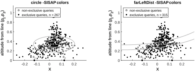
Figure 11: Two more binary partitions, based now on median distance from arbitrary points in the plane (centre and top-left respectively); we have not yet found a use for these but include the diagrams to make the point that any such partition may be used.

It can be seen that, in this case, partitioning the plane according to the height of individual points above the X-axis is the more effective strategy. The disadvantage with this is that a little more calculation is required to plot the height of the point, rather than its offset from the Y-axis; however this is a very minor effect when significantly more distance calculations can be avoided.

Figures 9 and 10 illustrate more techical analyses of the point cloud, using Principle Component Analysis (PCA) and Linear Regression (LR) respectively. Either technique can be used along one of two axes in a two-dimensional space as illustrated. In Section 4 we explain in the orthogonal linear regression technique in detail, and give experimental results showing its value as the best way to construct a balanced search tree over this data.

Finally we give the illustrations in Figure 11 to make the points that any partition of the plane can be used for this purpose. We have not yet found a compelling use for either partition, however this would depend on the nature of an individual non-uniform data set.

3.5. Balance

One further area of investigation, not yet performed, would be the effect of controlling the balance, which once again is arbitrarily possible simply by selecting different offset values. In general this will increase the probability of exclusion at cost of excluding smaller subsets of the data, and the effectiveness will depend on the individual distributions of the different strategies.

4. The Linear Regression Tree

In this Section we revisit a key observation of Section 3, and in particular Section 3.4, where we pointed out that any partition of the two-dimensional projected plane may be used to form an indexing mechanism. Up to this point we have restricted the use to simple Hilbert partitioning, where the data is divided only according to the nearest reference point. Here, we demonstrate a more flexible approach.

Figure 10 shows a scatter plot resulting from an arbitrary choice of reference points for the SISAP colors data set. Although the pattern is not atypical, observation shows that the individual distribution shape is significantly affected by the choice of reference points and, more subtly, by the subset of data points that is to be stored at a given tree node; although a high-dimensional space implies that these would not necessarily have a strong regional identity, this factor does visibly affect the relative mean distances to the reference points.

The partitions shown within the figure are based on the best-fit straight line which can be plotted through the points in two dimensions. This is parallel to the lines drawn in the right-hand figure. As this is calculated using the least-mean-squares algorithm, it is reasonable to assume that the perpendicular partition, shown in the left-hand diagram, will in general improve the spread of the data points and thus form a better partition for indexing5.

To test this strategy, we define the Linear Regression Tree (LRT), which is a binary tree built recursively over a datasetS as follows. We select two reference points p1, p2 at each node. Each child node of the tree shares one reference points with its parents, as done in the Monotonous Bisector Tree [11]. We used the tetrahedral projection based onp1andp2 to embed the data points onto a 2D plane, and we compute the best-fit linel through the projected points (or a subset of them) using a least squares minimization. Then, we rotate the 2D data points around the X-intercept of the linel, so that the new X-axis coincides with the linel, and we split the data at the median X coordinate of the rotated space.

Algorithm 1 and 3 give the simplest algorithms for constructing, and query-ing a balanced version of the LRT.

We compute the best fitting linelthrough the points{(xi, yi)}Ni=1as the line y=mx+b that best fits the sample in the sense that the sum of the squared

5_{As shown above, PCA seems to give a better spread than LR; for the moment we have}

Input :A⊂S, p1∈S

Output: Node: N=hp1, p2, δ, θ, h, Nleft, Nrightiwhere

{p1, p2} ⊂U, δ∈R, θ∈[0,2π), h∈R,{Nleft, Nright} ⊂Node

1 Selectp2 fromA;

2 if |A|>2then

3 A←Ar{p1, p2};

4 Ae←2Dproject(A, p1, p2);

5 (θ, h)←GetRotationAngle(Ae);// Calculate the rotation angle θ, and

the X-intercepts (h,0), that minimize the squared errors of the

y-coordinates following the rotation transformation

6 RotatedP oints← ∅;

7 foreach sej inAeido

8 rj←Rotate(sej, θ, h) ;// rj= (rj.x, rj.y)∈R

2

9 RotatedP oints←RotatedP oints∪ {rj}

10 end

11 δ←median{rj.x|rj∈RotatedP oints};// Find the median value of

the x-coordinate of the rotated points

12 Aleft← {sj∈A|rj.x, < δ};

13 Aright← {sj∈A|rj.x,≥δ};

14 Nleft←CreateNode(Aleft,p1);

15 Nright←CreateNode(Aright,p1);

16 N← hp1, p2, δ, θ, h, Nleft, Nrighti;

17 end

Algorithm 1: CreateNode (LRT balanced)

errors between theyi and the line valuesmxi+bis minimized. The fitting line

is easily computed asy−y¯=m(x−¯x) where ¯x=PN

i=1xi/N, ¯y=

PN

i=1yi/N, and

m=

PN

i=1(xi−x)(y¯ i−y)¯

PN

i=1(xi−x)¯ 2

. (1)

Then, we rotate the data points by angle θ = arctan(m) around the X-intercept (h,0), whereh= ¯x−y/m:¯

rx= (x−h) cos(θ)−ysin(θ) (2)

ry= (x−h) sin(θ) +ycos(θ). (3)

Input :A⊂S, p1, p2∈S

Output: SetAe⊂_R2

1 Ae← ∅;

2 foreach sj inAdo

3 Calculate the 2D embedded points_ej as the apex of the triangle defined by

baseline (0,−d(p1, p2)/2)−(0, d(p1, p2)/2), with left side lengthd(sj, p1)

and right sided(sj, p2);

4 Ae←Ae∪ {s_ej};

5 end

Algorithm 2: 2Dproject (2D projection ofA based onp1, p2)

Input :q∈U, t∈R, N=hp1, p2, δ, θ, h, Nleft, Nrighti ∈Node

Output: Result setR={s∈S|d(s, q)≤t}

1 R← ∅;

2 if d(q, p1)≤tthen

3 R←R∪ {p1};

4 end

5 if d(q, p2)≤tthen

6 R←R∪ {p2};

7 end

8 e

q←2Dproject({q}, p1, p2);

9 rq= Rotate(qe,θ,h); 10 if rq.x < δ−tthen

11 R←R∪Query(q, Nleft);

12 else

13 if rq.x > δ+tthen

14 R←R∪Query(q, Nright);

15 else

16 R←R∪Query(q, Nleft);

17 R←R∪Query(q, Nright);

18 end

19 end

0.052 0.083 0.131 Threshold 2000 4000 6000 8000 10000 12000 14000 16000 18000 20000 22000

no. of distance calculations

SISAP "colors" data set

MonPT-Balanced/ Far refs LRT-Balanced/ Far refs MonPT/ Far refs

0.052 0.083 0.131

Threshold 2000 4000 6000 8000 10000 12000 14000 16000 18000 20000 22000

no. of distance calculations

SISAP "colors" data set

MonPT-Balanced/ Rand refs LRT-Balanced/ Rand refs MonPT/ Rand refs

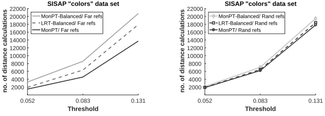
Figure 12: Colors –Monotone Tree (MonPT), Linear Regression Tree (LRT), and Balanced Monotone Tree with two different reference point selection strategies

0.12 0.285 0.53

Threshold 1000 2000 3000 4000 5000 6000 7000 8000

no. of distance calculations

SISAP "nasa" data set

MonPT-Balanced/ Far refs LRT-Balanced/ Far refs MonPT/ Far refs

0.12 0.285 0.53

Threshold 1000 2000 3000 4000 5000 6000 7000 8000

no. of distance calculations

SISAP "nasa" data set

MonPT-Balanced/ Rand refs LRT-Balanced/ Rand refs MonPT/ Rand refs

Figure 13: Nasa –Monotone Tree (MonPT), Linear Regression Tree (LRT), and Balanced Monotone Tree with two different reference point selection strategies

from within the data subset used to construct that node that is the furthest distance from the ancestor node.

The fair comparison is of the two balanced trees, and it can be seen that the Linear Regression Tree always outperforms the simple balanced tree.

The unbalanced tree however is always the best performer over this data set. Reasons for this are not altogether clear. However we believe this is worth reporting for sake of further investigation: in this domain, successful analysis of these reasons should lead to the ability to mimic them and deterministically produce a tree with still better performance.

In some of the further experiments performed in Section 7 we find that the Linear Regression Tree performs best out of all the mechanisms tested. This seems to be for large data sets which have significant non-uniformity, searching with smaller thresholds.

5. Hyperplane Partition Indexes and the Four-Point Property

over a range of hyperplane indexing structures. This is important in the light of the preceding discussion as, having established that issues such as balance and separation of reference points have quite different consequences, we need to understand the best indexing structure for taking advantage of the increased tractability. It is certainly not reasonable to assume that the best indexing structures for metric spaces will also the the best for supermetric spaces.

The best recorded general performance for an exact-search partition-based indexing structure, before the identification of using the four-point property within an exclusion mechanism, derives from the Distal Spatial Approximation Tree (DiSAT) [3]. This is therefore the obvious comparison to make between using normal metric properties and the four-point property over a space which has both properties; it allows the exactly same data structure to be measured with the different exclusion algorithms and in this sense is a very fair comparison. This comparison has been made in [1] and a significant improvement shown for using the four-point property: for the SISAP benchmark data sets, at the lower thresholds, typically around half the number of distance calculations are required when the four-point property is used over the same search index.

However, given the observations above on the different relative importance of the choice of reference point, it may be that the same data structure does not give the best performance when used for a supermetric space; the main differentiation between previous versions of the Spatial Approximation Tree (SAT) index and the DiSAT is the choice of widely separated reference points at higher levels of the tree, and it is therefore possible that different optimising factors will occur within a supermetric space.

We therefore performed a thorough investigation on a number of differ-ent exact-search hyperplane tree structures, taking each possible orthogonal attribute separately and testing all possible combinations with both Hyperbolic and Hilbert Exclusion strategies to determine the best data structure for use in a supermetric space.

5.1. Partition Trees

The basic structure of a partition tree is a recursively defined, n-ary tree. Each child of a parent node is governed by a single reference point, and every element of the data set contained below any parent node is associated with the child node whose reference point is closest to that element. The basic construction of a partition tree is given in Algorithm 4.

Query of such a tree allows a number of exclusion possibilities. Most simply, the distance from the query to each reference point is calculated; any partition may be excluded if this distance is greater than the cover radius (cri) added to

Input : Finite set of data objectsS⊆U

Output: Node of arityn: N=h{p1, . . . , pn},{N1, . . . , Nn},{cr1, . . . , crn}i

wherepj∈S,Nj∈Node,crj∈Rfor alljfrom 1 ton

1 if |S| ≤nthen

2 N← hS,∅,∅i //leaf node

3 else

4 select{p1, . . . , pn}fromS;

5 foreachpiin{p1, . . . , pn}do

6 Si←

s∈Sr{p1, . . . , pn}|i= arg minj=1,...,nd(s, pj) ;

7 cri←mins∈S_id(s, pi);

8 Nx←CreateNode(Si);

9 end

10 N← h{p1, . . . , pn},{N1, . . . , Nn},{cr1, . . . , crn}i

11 end

Algorithm 4: CreateNode

Input :N =h{p1, . . . , pn},{N1, . . . , Nn},{cr1, . . . , crn}i ∈N ode, q∈U, t∈R

Output: setR={r∈S|d(q, r)≤t})

1 R← ∅;

2 foreachpiin{p1, . . . , pn}do

3 di←d(q, pi);

4 if di≤tthen

5 R←R∪ {pi}

6 end

7 end

8 if {N1, . . . , Nn} 6=∅then

9 Excs← ∅;

10 foreachpiin{p1, . . . , pn}do

11 if d(q, pi)≥cri+tthen

12 Excs←Excs∪ {i}

13 end

14 forpj∈ {p1, . . . , pn}rpido

15 if d(q, pi)−d(q, pj)>2tthen

16 Excs←Excs∪ {i}

17 end

18 end

19 end

20 foreachiin{1, . . . , n}rExcsdo

21 R←R∪QueryNode(Ni)

22 end

23 end

d(q, pi)−d(q, pj)>2t

is replaced by

d(q, pi)2−d(q, pj)2

d(pi, pj)

>2t

The extra required term,d(pi, pj) can be calculated at build time and stored

for a small extra space cost, explained in Section 6.

The many different types of tree we tested are differentiated by how the reference set is chosen at each tree node. We tested a number of variants of trees according to the following largely orthogonal principles:

Pure SAT property Each node of a purely-formed Spatial Approximation

Tree has the property that no values from within the data set are closer to the “centre” node (the reference point in the parent node associated with each child node) than they are to any of the reference points one level down within the tree. This principle of construction allows further exclusion possibilities, as during a query the maximum distance between the query and any higher-level reference points may be passed recursively; if this distance is greater than max(d(q, pj)), i6=jthen it may be used to

attempt to excludeNi from the search.

Any serial selection of reference points requires, as each node is con-structed, that any point closer to the centre node than any previously selected reference point is added to the set of reference points. As pointed out by the authors of [3] the construction has very different properties depending on the order in which the contained set is considered.

Two variants of such “pure” SATs were tested; forsat pure, we considered the data set of inclusion in the reference set in order of distance from the centre node, and forsat distal purewe considered them in reverse order. We also tried some hybrids but did not discover any interesting results, so these are not reported.

For using the Hilbert Exclusion mechanism for trees with this pure SAT property, the distances to ancestor nodes can still be used, but (i) all distances need to be recursively passed, rather than just the maximum, and (ii) at build time, all distances from each pi to all ancestors also

require to be calculated and stored. This is because the Hilbert exclusion condition requires all three distances among any two reference points and the query to be known. We tested both construction and query for any extra cost associated with this extra information flow, and it was found to be insignificant.

SAT construction Faster versions of SAT as reported in [3] do not maintain

algorithm (traversingS according to an imposed order and adding refer-ence points whenever they are closer to the centre node than any existing reference point), however this process is terminated according to the num-ber of reference points selected. This is because the pure SAT algorithm, applied to the distal ordering of values from the centre, leads to very wide, shallow trees which do not lead to good performance when using Hyper-bolic exclusion. The extra exclusion possibilities from using the parent reference point distances are lost, but wider separation of reference points was found to lead to more exclusions.

Therefore the extra factor of maximum branching factor is considered. We considered two; sat distal fixed uses a fixed value of 4, found in [3] to give good performance, andsat distal loguses a dynamic value selected according to the data size, chosen not to exceed the natural logarithm of the data size, thus reducing as the tree is descended.

Choice of the centre point for the head node, for best performance, is described in [3] as being acheived by choice of an outlier, this giving the SATout class of algorithm (sat global fixedandsat global log); we

con-firmed this result and therefore reused this strategy for all of our experi-ments.

Finally, the SATglobclass of tree uses a single ordering for consideration of

reference point selection, based on an ordering of the whole data set from the centre node of the entire tree, rather than the centre of each node.

Non-SAT construction Finally, we considered a number of partition trees

(hpt *) where the choice of reference point was made independently of their distances from the parent reference point. Three arities were chosen;

fixed andlogarithmicas above, but also abinary version was constructed. Two strategies for reference point selection were used to fill these arities:

random selection, and one using theFFT algorithm [23, 24].

5.2. Experimental Procedure

The above classification leads to the following set of tree structures used for experiments: sat pure, sat distal pure, sat distal fixed, sat distal log, sat global fixed, sat global log , hpt fft binary, hpt fft fixed, hpt fft log, hpt random binary, hpt random fixed, hpt random log – each of these should have a clear meaning given the above description. For each tree, both Hyper-bolic and Hilbert exclusion mechanisms were tested, leading to a total of 24 different search indexes.

Each was tested against the SISAP benchmark data setscolors andnasa[4] using Euclidean distance. For each test, three different query thresholds were used as is standard for the SISAP benchmark sets. 10% of the data was ran-domly removed to act as a query set.

Data Set # elements feature dim dist

SISAP Colors [4] 112,682 Color Histograms 112 `2

SISAP Nasa [4, 25] 40,150 PCA-red. Color Histograms 20 `2

Table 2: Data Sets Statistics

Data Set t0 (0.01%) t1 (0.1%) t2(1%)

nasa 0.120 0.285 0.530

colors 0.052 0.083 0.131

Table 3: Experimental threshold values that return around 0.01%, 0.1% and 1% of the data sets

For sake of space, we give only the main results: for each index, and each data set, we give the number of distances per query at a single query threshold. We also tested query times; in all cases the number of distances was directly proportional to the query time, which is not surprising as all of the data sets used fit comfortably within the main memory and this is by far the dominant cost of the query. It is useful to confirm however that the extra administrative cost associated with the Hilbert exclusion is negligible with respect to distance costs.

All tests were executed in Java, using the same Java abstract tree construc-tion and query classes, specialised only according to the reference point selecconstruc-tion strategy and query-time exclusion strategy. As a final semantic check, all results were cross-checked against a serial (exhaustive) search to ensure consistency and therefore correctness. All code used is available in a public repository6_.

For each test, multiple tree builds were performed and mean values are presented. For each build, the data was presented in randomised order, as the order of selection during tree build can have a significant serendipitous effect on performance. Tests were repeated until the standard error of the mean was ≤ 1%, which implies that all of the differences reported are statistically significant.

Results are shown in Figure 14 and 15.

5.3. Analysis

The most obvious conclusion is that the supermetric exclusion always gives better performance; while this is actually a guarantee as shown in [1] the inter-esting point is the magnitude of the improvement, which in some cases is quite startling.

SISAP colors

sat_pure

sat_distal_puresat_distal_fixedsat_distal_log_{sat_global_fixed}sat_global_loghpt_fft_binary

hpt_fft_fixedhpt_fft_log

hpt_random_binaryhpt_random_fixed

0 5000 10000 15000 20000

Average number of distances per query

Hilbert Exclusion Hyperbolic Exclusion

Figure 14: Partition Trees: SISAPcolors at thresholdt0

SISAP nasa

sat_pure

sat_distal_puresat_distal_fixedsat_distal_log_{sat_global_fixed}sat_global_loghpt_fft_binary

hpt_fft_fixedhpt_fft_log

hpt_random_binaryhpt_random_fixed

0 1000 2000 3000 4000

Average number of distances per query

Hilbert Exclusion Hyperbolic Exclusion

Although not quite the absolute best performance, the greatest improvement is in the pure SAT indexes, both classic and distal variants which in fact seem to give around the same performance. This is worthy of further study; as mentioned, the shape of these trees is very different, the classic SAT giving a relatively small branching factor against a very large branching factor at the higher levels of the distal SAT. The inventors of the distal SAT compromised the SAT property early on, presumably because performance was badly affected by this property. Using the four-point property seems to overcome this. As these data sets are relatively small there is no real advantage to a shallow tree, but this may well be different with very large data.

The lack of variance for the four-point exclusion across all the different struc-tures is also notable; this confirms our earlier hypothesis that the actual exclu-sion power of the Hilbert mechanism is much less affected by the choice of reference point, and certainly confirms that putting huge computational re-sources into building expensive data structures may be far less worthwhile in this context.

Finally, we note the best performance data structure considered here, the log-sized hyperplane tree using the FFT algorithm to choose reference points. Paradoxically, this is one of the simplest, and fastest, structures to construct. It is likely that using a more sophisticated cluster-finding algorithm such as k-means or k-medoids may perform a little better, although at much higher tree build cost; given the rather small incremental improvement however of FFT over random, we are not convinced that this would be worthwhile in many cases.

And as a last word: we note that the values of 1,704 distance measurements per query achieved over the SISAPcolors data set, and 171 measurements per query over the nasa data set are, for the moment, new performance records against this benchmark.

6. The Cost of Hilbert Exclusion

While it has been shown that Hilbert Exclusion performs better than Hy-perbolic in run-time cost, there is an extra space cost involved as more infor-mation is required: the distance between the reference points is required for the query-time exclusion calculations, where it is not for the hyperbolic exclusion calculation. It is thus important to assess the extra overhead in time and space. In all cases, the choice of reference points is made during the building of the index structure; therefore it is possible for the distances to be calculated at build time and stored. Feasibly, they could instead be calculated at query time if the storage overhead was relatively great compared with the extra query-time cost; however here we show that it is not.

In the case of binary trees, the extra space overhead is a single distance value, or 4 bytes7, per node. Even the leanest tree implementation will have a

per-7_{as the value is only used for additive arithmetic and is not critical for correctness, single}

node space overhead much greater than this, although of course this depends on the language and implementation tactics used. A modern JVM has a minimum object overhead of 16 bytes, along with a further 32 bytes to store pointers to two subtrees even before any other node information is considered, such as object ids for the reference objects, cover radii, etc. Realistically the extra overhead is likely to be much less than 10%; given the further invariant that the number of internal tree nodes is less than one-half the number of data8_, and each data object is likely to be much bigger than a tree node, the space overhead is minimal and unlikely to be significant in any realistic scenario.

For general hyperplane trees with more than two reference points the over-head is potentially greater as all inter-reference point distances are required, giving a theoretical O(n2_{) space cost. Pragmatically however the values of n} involved are fairly small; furthermore as we are dealing with proper distances we only need store the upper triangular matrix, so the space overhead is n₂

rather thann2_{. For example, in [3] the authors observe that a DiSAT branching factor} of 4 gives optimal performance in some contexts; here we can replace theO(n2) observation with a constant value of 6, i.e. 24 bytes per tree node. In the case of a quadtree, the number of internal tree nodes will be less than approximately a third of the data size, giving a maximum overhead of less than 8 bytes per data object

Finally we consider the log-sized node strategy, where the number of refer-ence points at each tree node is approximately the log of the volume of data stored below the node. This leads to much bigger overhead at the root of the tree; for example the root node of a tree for 1010 _{data objects has 23 reference} points, requiring 1KByte of overhead. However these trees are correspondingly shallower, and the node size decreases rapidly as the tree extends downwards. There is a recurrence relation to estimate the space overhead in bytes for a balanced tree:

overhead(N) = 0, N ≤2

overhead(N) =

_|p|

2

×4 +|p| ×overhead(N_|p|−|p|) where |p| = blogNc

When applied to any large size the overhead turns out to be only around one byte per data object.

There is also clearly an extra run-time cost in construction, from the mea-surement of extra distances. This is of much less concern; in any partition strategy, for every node built, there is a requirement to measure the distances between every data item below the level of that node against all of the refer-ence points. Without further analysis it seems clear that the extra overhead of measuring the distances among the nodes is relatively trivial.

Experimental evidence supports the notion that the extra overhead, in both

time and space, is insignificant, independent of the strategy used. We have tried to detect significant differences in either construction time or space in the large experiments described in Section 7, but in all cases the differences have been hidden in the noise caused by the introduction of randomisation to the construction process.

7. Spaces with Larger Scale and Higher Dimensionality

In this section we investigate extending the use of the supermetric property to larger and higher-dimensional data sets. The purpose is to explore how the behaviour of the mechanisms, which have been shown to give good results over (relatively) small benchmark sets, alters with sets that are inherently more difficult to index.

We perform three types of test to demonstrate these behaviours:

increasing dimensionality In these tests, we generate evenly-spaced points

within generated Euclidean spaces of increasing dimension and test Hy-perbolic and Hilbert exclusion mechanisms for query performance. These tests show the effect that increasing dimensionality has on the relative performance; pragmatically we show that at the point where increasing dimensionality starts to make search intractable, the use of Hilbert exclu-sion gives an extra 2-3 dimenexclu-sions for the same level of performance.

“real-world” high-dimensional data In these tests we use GIST

represen-tations of the MIR-Flickr [26] data set of one million images to perform a near-duplicate search; these are large data comprising 480 floating-point numbers, tested with various metrics. These tests show that the efficacy of Hilbert exclusion does not seem to be affected by the choice of metric.

increasingly large data sets In these tests we use 80 dimensional MPEG-7

Edge Histogram data taken from the CoPhIR [27] images set . Tests are made over increasingly large subsets (between 1 and 16 million images) to show how the mechanisms scale as the data size increases.

7.1. Increasing Dimensions

For each dimension between 2 and 20 inclusive, evenly distributed Carte-sian points were generated within the unit hypercube. For each dimension, a Euclidean space of one million data points was generated, and one thousand threshold queries were executed over each space. At each dimension a threshold was selected with a radius calculated to give one-millionth of the volume of the unit hypercube9_.

9_{For dimensionn, radiusr}

n=

Γ(n₂+1)

π n

2

0% 5% 10% 15% 20% 25% 30% 35% 40% 45% 50%

2 3 4 5 6 7 8 9 10 11 12 13 14 15 16 17 18 19 20

Pr

oportion of Da

ta Acc

ess

ed

Dimension

Euclidean spaces of increasing dimension

hpt_random_log hpt_fft_log

hpt_random_log - Hilbert hpt_fft_log - Hilbert

0.0% 0.5% 1.0% 1.5% 2.0% 2.5% 3.0% 3.5% 4.0% 4.5% 5.0%

2 3 4 5 6 7 8 9 10 11 12 13 14 15 16 17 18 19 20

Pr

oportion of Da

ta Acc

ess

ed

Dimension

Euclidean spaces of increasing dimension

hpt_random_log hpt_fft_log

hpt_random_log - Hilbert hpt_fft_log - Hilbert

Figure 16: The effect of increasing dimensions on the four HPT mechanisms. The right-hand side is a magnified version of the left, allowing the very significant performance differences at lower dimensions to be seen better.

After first confirming that the log-sized hyperplane partition tree is still the most efficient index at all dimensions, measurements were made for four variants to establish the added value of the Hilbert exclusion mechanism. Trees were built using both random and FFT selection strategies for each node, and for both of these variants, querying was performed with, and without, the Hilbert exclusion mechanism. As previously noted, the same instance of the built data structure can be used in either way, as long as the metric has the four-point property. The figure recorded is the number of distance calculations required per query over the data set; at each dimension, each experiment was repeated until the standard error of the mean was less than 1%.

Figure 16 shows the outcomes. It can be seen that, across all dimensions, the FFT variant is better than a random choice of reference points for either exclusion mechanism, and more significantly for our purposes that the Hilbert exclusion variant is substantially better than the Hyperbolic.

Metric IDIM Unit cost t1 t2 t3 t4 t5

Euclidean 14.3 0.0016 0.016 0.044 0.070 0.096 0.125

Cosine 15.5 0.0013 0.006 0.016 0.027 0.037 0.048

Jensen-Shannon 10.8 0.017 0.005 0.011 0.018 0.024 0.032

Triangular 12.1 0.0029 0.006 0.013 0.021 0.029 0.037

Table 4: GIST: IDIM, cost per distance measurement, and thresholds used

four-fold increase in performance.

The tree hpt fft log (FFT pivot selection) using the Hilbert exclusion mechanism shows quite similar performance to the tree hpt random log (ran-dom pivot selection) using the Hyperbolic exclusion mechanism; although sub-ject to heuristics and uncertaintly, in our experiments the FFT-based choice of reference points gives a build cost of around five times that of the hyper-plane tree with randomly selected reference points, and indeed the latter is one of the cheapest indexing mechanisms to build; if build time is an important consideration, this could give the best compromise.

An alternative view of the results is to consider where the different lines cross a given horizontal boundary in the chart. For example, if a particular situation indicates that accessing no more than 2.5% of the data is required to give sufficient performance, than this can be achieved with a data set whose dimensionality is around 13 using FFT and Hilbert exclusion, whereas only around 10 can be achieved, from the same indexing mechanism, without these.

7.2. MirFlickr/GIST and Near-Duplicate Detection

In these experiments we test a large data set for a real-world purpose, namely the detection of near-duplicate images. In previous work we have shown the use of the GIST characterisation gives the best tractable test for near-duplicate image detection within large sets of images [28]; these tests are inherently ex-pensive because of the data size, and efficient similarity search is important to give tractability. Each GIST object10 _{comprises 480 dimensions of floating} point numbers, which using IEEE single-precision format gives an object size of almost 2KBytes per object, i.e. just under 2GBytes per million images.

While the intrinsic dimensionality of these spaces is relatively high – around 10-15 depending on the metric – the required search thresholds are quite low, therefore giving a nice example of spaces where metric search is particularly appropriate for the task in hand.

We used the Mir-Flickr [26] set of one million images and generated GIST representations. We have previously demonstrated the use of this collection as a benchmark for near-duplicate image detection; the collection by chance contains

10_{using GIST parameters: 4 windows, 6 scales and 5 orientations per scale, taken from a}

0% 1% 2% 3% 4% 5% 6% 7%

t1 t2 t3 t4 t5

Pr

oportion of Da

ta Acc

ess

ed

threshold MirFlickr- GIST

euc - Hyperbolic tri - Hyperbolic jsd - Hyperbolic cos - Hyperbolic euc - Hilbert tri - Hilbert jsd - Hilbert cos - Hilbert

0 0.5 1 1.5 2 2.5 3 3.5 4 4.5

t1 t2 t3 t4 t5

Impr

o

vem

en

t

threshold

Improvement: Hilbert over Hyperbolic

euc cos jsd tri

Figure 17: Four different metrics over GIST data at different thresholds, with and without using Hilbert exclusion.

around 2,000 clusters of near-duplicate images which we have identified, allowing both sensitivity and specificity to be accurately tested for different metrics and thresholds [29]. The GIST representations can be used for this purpose with any of Euclidean, Cosine, or Jensen-Shannon distances. A key aspect of such classification functions with very large collections is their specificity, which must be high to avoid very large numbers of false positives. All of these tests maintain high specificity up to a sensitivity of around 50%; to test the efficiency gains of the Hilbert Exclusion we therefore tested searches over the collection at five different thresholds, representing for each metric sensitivity of 10% to 50%, after which point a fast drop-off in specificity occurs. Table 4 gives, for each metric, the intrinsic dimensionality, the mean cost per distance measurement in milliseconds, and the thresholds used to search.

to be almost exactly directly proportional and so only the number of distance calculations are presented, given as the mean proportion of the total data size tested per query.

Figure 17 shows results from these experiments. It appears that the advan-tage given by using the Hilbert exclusion mechanism is relatively independent of the metric being considered. In all cases it is highly significant, giving a performance improvement of 2.5 to 3 times for all metrics, even at the top end of the thresholds tested.

7.3. Increasing Scale

In these experiments, we investigate how the advantages shown by the Hilbert property are affected by the scale of the data. To measure this, we used MPEG-7 Edge Histogram descriptors extracted from the CoPhIR [27] image data set, using the first 80 dimensions of the raw data. We queried increasingly large subsets of the data, ranging from one million to sixteen million images, to test the scalability of the different search mechanisms. Results are reported for Euclidean distance; we repeated the tests using other metrics and found no interesting differences.

We sampled 109_{randomly selected distances to measure IDIM and to choose} search thresholds; the IDIM of the data was measured as 7.5, and three thresh-olds were selected to return 10−8_{, 10}−7_{and 10}−6_{of the data per query}11_{; these} thresholds are small but this is appropriate as data becomes larger.

With relatively smaller threshold and larger data we did not make assump-tions about which mechanisms of those tested earlier would perform best; we tried them all, and report here the most interesting representative results. As there is some anecdotal evidence that single-pivot strategies can be more ef-fective that hyperplane partitions as thresholds decrease, we also included a vantage point tree [30] in the tests. For each search structure, we performed 1,000 queries selected randomly from a different part of the set and measured the number of distance calculations performed; we present these as a proportion of the data access per query.

Figure 18 shows the outcomes. We present results for: log-sized hyperplane trees, with Hilbert and Hyperbolic exclusion; monotone (binary, unbalanced) hyperplane trees, again with Hilbert and Hyperbolic exclusion; a balanced van-tage point tree, and a linear regression tree. Reference points for the log-sized hyperplane trees are selected using FFT, and for the monotone binary trees by simply selecting the furthest object from the inherited reference point.

For all mechanisms and thresholds, it can be seen that as the size of the dataset increases, the proportion of data accessed decreases. The rate of this decrease demonstrates scalability of the mechanism. The value of the Hilbert exclusion is very marked, especially with the larger threshold values. It is inter-esting to note that the vantage point tree performs very well with a very small threshold, but is relatively much worse as the thresholds get larger. Although a