A Dynamic Prescriptive Maintenance Model
Considering System Aging and Degradation
BIN LIU 1, (Member, IEEE), JING LIN 2, (Member, IEEE),
LIANGWEI ZHANG 3, AND UDAY KUMAR2
1Department of Management Science, University of Strathclyde, Glasgow G1 1XQ, U.K.
2Division of Operation and Maintenance Engineering, Luleå University of Technology, 971 87 Luleå, Sweden 3Department of Industrial Engineering, Dongguan University of Technology, Dongguan 523808, China Corresponding author: Liangwei Zhang ([email protected])
This work was supported in part by the Luleå Railway Research Centre (Järnvägstekniskt Centrum), Sweden, in part by the Swedish Transport Administration (Trafikverket), in part by a project by the NSFC under Grant 71801045, and in part by the Youth Innovative Talent Project from the Department of Education of Guangdong Province, China, under Grant 2017KQNCX191.
ABSTRACT This paper develops a dynamic maintenance strategy for a system subject to aging and degradation. The influence of degradation level and aging on system failure rate is modeled in an additive way. Based on the observed degradation level at the inspection, repair or replacement is carried out upon the system. Previous researches assume that repair will always lead to an improvement in the health condition of the system. However, in our study, repair reduces the system age but on the other hand, increases the degradation level. Considering the two-fold influence of maintenance actions, we perform reliability analysis on system reliability as a first step. The evolution of system reliability serves as a foundation for establishing the maintenance model. The optimal maintenance strategy is achieved by minimizing the long-run cost rate in terms of the repair cycle. At each inspection, the parameters of the degradation processes are updated with maximum a posteriori estimation when a new observation arrives. The effectiveness of the proposed model is illustrated through a case study of locomotive wheel-sets. The maintenance model considers the influence of degradation and aging on system failure and dynamically determines the optimal inspection time, which is more flexible than traditional stationary maintenance strategies and can provide better performance in the field.
INDEX TERMS Aging and degradation process, dynamic maintenance strategy, locomotive wheel-sets, prescriptive maintenance, sequential schedule.
I. INTRODUCTION
With the increasing integration of systems, maintenance strategies are placing more emphasis on techno-economic than technological considerations. Existing maintenance strategies include time-based maintenance, where nance actions are performed at failure (corrective mainte-nance) or based on system age (age-based maintemainte-nance), and condition-based maintenance, where maintenance decisions are provided based on the health condition of the system.
Prescriptive maintenance has gained popularity in recent years. It extends the concept of failure prediction [1], [2] by predicting maintenance measures and prescribing a course of actions based on the historical and incoming real-time data. Prescriptive maintenance strategies are updated based on the
The associate editor coordinating the review of this manuscript and approving it for publication was Yu Wang.
observed/predicted degradation parameters and system state, whereas in conventional time-based maintenance, decisions only rely on historical data without considering updates. In this paper, we develop a dynamic maintenance model able to sequentially determine the optimal inspection time based on the system health condition and provide flexible maintenance advices.
which is usually characterized by a Markov or semi-Markov chain [3]–[7]. The disadvantage of Markov or semi-Markov models lies in the arbitrary classification of the system states and fails to fully characterize its degradation evolution.
Increasingly improved sensing technologies enable accu-rate monitoring of the system state, prompting the use of a continuous degradation model. Usually, the continuous degradation processes are described by stochastic process models or general path models [8]–[10]. The Lévy pro-cess is frequently used because of its mathematical prop-erties and explicit physical interpretations, among which the Gamma process, Wiener process, and inverse Gaussian process have widely appeared in the reliability and mainte-nance literature. Although the Wiener process is extensively used for reliability modeling and maintenance optimization (e.g., [11]–[14]), it is a non-monotone process and fails to describe several deterioration processes in practice, such as the crack growth or wear process. On the other hand, with the property of monotonic independent increments, the Gamma process and inverse Gaussian process can overcome this disadvantage [15]–[17]. Reference [18] provided a compre-hensive survey of the use of the Gamma process in reliability and maintenance strategies. In [17], the inverse Gaussian pro-cess was investigated as a degradation model and the physical mechanism was interpreted as a limiting compound Poisson process. Novel BN/DBN-based methodologies are developed for degradation modeling of components and systems [19].
In spite of the popularity of degradation models in relia-bility and maintenance modeling, an implicit assumption of the existing studies is that a failure occurs when the degrada-tion level exceeds a specific threshold (soft failure). Yes this assumption is increasingly challenged since many systems fail before hitting the failure threshold in reality [20]–[24]. For locomotive wheels, usually the diameter of a wheel indi-cates the degradation level, where a soft failure is defined when the diameter reduces to a pre-specified threshold. How-ever, during operation, wheels are reprofiled occasionally because of the increased roughness, even if the wheel diam-eter remains above a tolerance level. Various factors exert impacts upon the roughness of the wheels, including the weather conditions, surface smoothness of the track and run-ning speed; any of these may cause sudden failure before the failure threshold is reached [25], [26]. Reduction of the wheel diameter through reprofiling also exacerbates the roughness. Another example is automobile tires. An automobile tire may fail suddenly because of a puncture before the wear reaches the failure threshold [27]. Reference [28] reported the limitation of the degradation-threshold failure model in the presence of continuous monitoring. When the system is subject to continuous monitoring, maintenance actions can always be implemented before the degradation level reaches the failure threshold, and this erroneously indicates that the system will never fail.
Motivated by the limitation of the degradation-threshold failure mechanism and the maintenance practices used for locomotive wheel-sets, we propose a maintenance strategy
that considers the impact of degradation and catastrophic failure. It is well recognized that system failure is depen-dent on both degradation and age [28]–[30]. Reference [29] proposed a class of degradation-threshold-shock models that take advantage of degradation information and failure data. Reference [28] developed a condition-based maintenance strategy under continuous monitoring; they proposed respec-tively an additive and a multiplicative model to describe the relationship between system failure rate and degradation level.
In this paper, we develop a maintenance model that jointly incorporates the effect of both aging and degradation. In this model, the degradation level and system age have an additive impact on system failure rate. At inspection, replacement is carried out if the degradation level of the system hits a toler-ance threshold and repair is implemented otherwise. Repair influences the system health condition in such a way that it reduces the system age to 0, but increases the degradation level. The degradation level and parameters are updated at inspections when new observation arrives. The maintenance strategy determines the optimal inspection time based on the updated degradation parameters and the degradation level after repair/replacement.
Our work differs from previous research in three aspects. First, we use a continuous stochastic process to describe system degradation, and we incorporate the joint influence of degradation and aging on system failure rate in an additive way. Second, we formulate a dynamic maintenance model as opposed to the static maintenance models in the literature; the parameters of the degradation process and the subsequent maintenance decisions are updated upon the arrival of new inspection data. Third, the effect of preventive maintenance action is twofold in our model: a reduction in system age and an increase in degradation level.
The rest of the article is organized as follows. Section II characterizes the degradation process and investigates system reliability. Section III describes the maintenance schedule and formulates a cost model as the maintenance criterion. Section IV discusses the procedure for estimating and updat-ing parameters. A case study of locomotive wheel-sets is presented in Section V to illustrate the proposed maintenance strategy. Finally, Section VI provides the concluding remarks and future research directions.
II. DEGRADATION PROCESS AND RELIABILITY EVALUATION
A. SYSTEM DEGRADATION
1X(t−l)=X(t)−X(l), follows a Gamma distribution with the probability density function (pdf)
f (x;α(t−l)β)= β
α(t−l) 0 (α(t−l))x
α(t−l)−1e−βxI
{x>0} (1) where0 (·)is the complete gamma function, andI{x>0}is the indicator function.
B. RELIABILITY EVALUATION
The system may experience sudden failure in addition to the continuous degradation process, where both system age and degradation level contribute to the increase of failure rate. Traditional age-based maintenance strategies fail to capture the heterogeneity of the operating systems since the failure rate is only dependent on system age. For example, for loco-motive wheels operating in different environments, such as the track condition, weather, and running speed, they may suffer heterogeneous failure rates even with identical age. Hence, modeling the failure rate as a function of system age and degradation level can better describe the failure mech-anism of real systems. Note that the impact of degradation lies in increasing the failure rate, while itself will not lead to system failure. Let λ (t,X(t))denote the failure rate at timetand system degradation levelX(t). Conditioned on the degradation path till timet,X0t = {X(s), 0≤s≤t}, system reliability is given as
R t|X0t=exp
−
Z t
0 λ (
s,X(s))ds
(2)
DenoteTf as the time to failure. The expectation of system
reliability is expressed as
¯
R(t)=PTf >t =E
exp
−
Z t
0 λ (
s,X(s))ds
(3)
In general, numerous forms ofλ (t,X(t))can be employed as long as it can capture the influence of system age and degradation level on the failure rate. In presence of historical data and physical mechanism, the specific form ofλ (t,X(t)) can be determined in detail. For simplicity, an additive model is used [28],
λ (t,X(t))=λ1(t)+λ2(X(t)) (4) Equation (4) implies the influence of system age and degra-dation level on the failure rate in an additive way. In particular, λ1(t) describes the age-dependent failure rate, andλ2(X(t)) depends on the degradation level.
For the failure rateλ2(X(t)), we assume a linear function in terms of the degradation levelX(t),λ2(X(t)) = γX(t), whereγ is a positive constant, scaling the impact of degra-dation level. Given the initial degradegra-dation level x0 and the linear formula ofλ2(X(t)), the system reliability is expressed as follows.
Proposition 1: For a system subject to an age- and degradation-dependent degradation process with an additive effect, system reliability is given as
¯
R(t;x0)=exp
−
Z t
0
λ1(s)+γx0+αlog(1+γs/β)ds
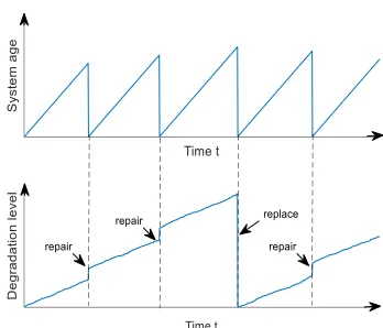
[image:3.576.329.503.60.209.2]
FIGURE 1. Evolution of system age and degradation level at maintenance actions.
Proof of the proposition is provided in the appendix. Note that the time to failureTf can be regarded as the first instance of a doubly stochastic process, with a stochastic intensity λ (t,X(t))that depends on both the degradation level and system age [29], [31].
Corollary 1:If the age-dependent failure rate is constant, λ1(t)=λ0, system reliability is then given as
¯
R(t;x0)=exp(−(λ0+γx0)t−α ((β/γ+t)log(1+γt/β)−t))
Corollary 1 can be readily obtained from the reliability function of Proposition 1.
III. MAINTENANCE SCHEDULING
In the proposed maintenance model, the system is subject to three maintenance actions, namely, inspection, repair, and replacement. Repair is implemented preventively to prevent the system from failure or correctively to restore the system from failure. Unlike the existing imperfect repair models, in the proposed model, the influence of repair is twofold. On one hand, repair reduces the system age but on the other hand, increases the degradation level. In the present main-tenance of locomotive wheels, the wheels are transported to the maintenance station for repair. During repair, they are reprofiled to restore them from anomaly. The reprofiling process diminishes the diameter of the wheels. In other words, the re-profiling process during repair increases the degrada-tion level. In this paper the sudden failure is referred to as an anomaly during operation.
A dynamic maintenance strategy is developed in this paper, wherein maintenance decisions have to be made at each inspection, including the time for the next inspectionti, and repair or replacement upon the system. Denote Xi− as the degradation level before theith repair andXi+the degradation level after repair. Let Yi be the increment of degradation
level at theith repair.Yiis assumed to be independent of the
degradation levelXi−and follows a Gaussian distribution with mean µand varianceσ2,Yi ∼ N µ, σ2
. With the above definition, we have
Xi+=Xi−+Yi
Xi−+1=Xi++1X(ti)
Let πi ∈ {0,1} denote the maintenance action at the ith inspection, where πi = 1 stands for replacement, and
πi=0 indicates repair. Replacement is carried out upon
the system when the degradation after repair reaches a pre-specified tolerance level, i.e.,
P xi−+Yi< ζ> η
whereζ is the threshold for replacement andηthe tolerance level. SinceYifollows a Gaussian distribution, it follows that
8 ζ −µ−x
− i
σ
!
> η
The maintenance action at the ith inspection can be obtained with simple algebra, given as
πi = (
0, ifxi−≥ζ −8−1(η)·σ −µ
1, otherwise (5)
Besides the maintenance actions at inspections, the deci-sion maker will also have to determine the time for the next inspection, ti, given the degradation level after repair
or replacement, Xi+. In addition, at each inspection where new degradation data arrive, the degradation parameters and system state are updated based on the arrival of new observa-tions. It is difficult to obtain a stationary optimal maintenance decision, since all possible observation values have to be con-sidered ahead of time [35]. As an approximation, we achieve the optimal maintenance decision by minimizing the expected average cost within a repair cycle.
The approximation model has two advantages. First, com-pared to a stationary maintenance model, the computational burden is significantly reduced. Second, the proposed one-repair-cycle optimization provides more flexibility for the optimal maintenance strategy. Although we can theoretically obtain the optimal inspection time based on the degradation process and observations, yet in practice, the actual mainte-nance time is influenced by the workload of the system and may deviate from the optimal maintenance time. In terms of actual maintenance time, the proposed model can be applied with a tiny modification of the repair cycle. The system should be maintained as close as possible to the optimal time to reduce the maintenance cost.
At the ith inspection, given the degradation level after repair,Xi+, the expected cost per unit time is provided as
CR ti;xi+
=E
c
i+cp·1{Tf≥ti} +cc·1{Tf<ti} +cdTd
ti
= ci+cp ¯
R(ti;xi+)+cc 1− ¯R(ti;xi+)
+cdE[Td]
ti (6)
whereci,cp, andccdenote respectively the cost of inspection,
preventive repair and corrective repair,cd is the downtime
per unit time, 1{·} is the indicator function, ti is the time
interval between theith and (i+1)th inspection, andTd is
the downtime. The expected downtime within the intervalti
can be obtained by conditioning on the degradation pathXti 0 and is given as
E[Td]=E Z ti
0
1−exp
−
Z t
0 λ (
s,X(s))ds
dt|Xti 0
(7)
A detailed derivation of the equation is provided in the appendix. Numerical approaches like Monte Carlo integra-tion can be employed to evaluated Equaintegra-tion (7). The optimal inspection timeti∗can be obtained as
ti∗=arg min
ti
CR ti;xi+ (8)
For the system degrades over time with small variance, we can approximate the expected downtimeE[Td] as
E[Td]≈ Z ti
0
1− ¯R(t;xi+)dt (9)
and the expected average costCR ti;xi+as
CR ti;xi+
≈ci+cc−(cc−cp) ¯
R(ti;xi+)+cdRti
0 1− ¯R(t;x
+ i )
dt
ti
(10)
For a degradation process with small variance, given the degradation level after reprofiling,xi+, the expected remain-ing useful life is denoted asν= −R∞
0 tdR¯(t;x
+
i ). In Fig. 2,
we plot the evolution of inspection time (repair or replace-ment time) to illustrate the maintenance scheduling process. The system is inspected (together with repair or replace-ment) at epochsi. After repair or replacement, the decision
[image:4.576.300.534.649.692.2]maker needs to decide the operating interval before the next inspection time (ti).
FIGURE 2. Sketch of maintenance schedule.
CR(ti)decreases withti, forti → 0+, and increases withti forti→ ∞.
A detailed proof of the corollary is given in the appendix. Corollary 2 indicates the existence of the optimal inspection time, ti∗. For ν > (ci +cc)/cd, when ti varies from zero
to infinity, the expected cost per unit time CR(ti)shows a
decreasing trend at the beginning and then an increasing time, thus implying thatti∗exists.
Based on the previous discussion, the maintenance sched-ule is summarized as follows:
1) Determine initial input: initial degradation level,
x0=0, and leti=0.
2) Calculate the optimal inspection time, ti∗ = arg min
ti
CR ti;xi+.
3) At theith inspection time, judge whether the degrada-tion level hits the tolerance level,xi− ≥ζ −8−1(η)· σ −µ. If so, replace the system and return to Step 1. Otherwise, repair takes place; leti=i+1 and jump to Step 4.
4) Given the degradation level after repair,xi++1, calculate the next inspection time,
ti∗+1=arg min
ti+1
CR ti+1;xi++1
and go to Step 3.
5) Output the optimal inspection time, ti∗, for i = 0,1,2, . . ..
IV. PARAMETER UPDATE AT INSPECTION
In this paper, it is assumed that the degradation level of the system is accurately observed, with no measurement error. The scale and shape parameters are updated at each inspection, when newly arrived data are observed. Let θ = (α, β)T be the set of distribution parameters. Suppose that
the prior distribution ofθis a bivariate Gaussian distribution,
θ∼N µθ,6, where
µθ = µα, µβT and 6=
σ2
α ρσασβ
ρσασβ σβ2
Denotep(θ) as the pdf of prior distribution. It follows that
p(θ)=
exp−1 2 θ−µθ
T
6−1 θ−µ
θ
√ 2π|6|
The prior distribution parameter, µθ, is obtained with historical data, by using the maximum likelihood estima-tion (MLE). Asymptotic methods are used to evaluate the uncertainty of the prior distribution. Under reasonably large sample sizes, the estimators of MLE can be well approxi-mated by a multivariate Gaussian distribution. Denoteθˆ as the MLE estimator of θ. The asymptotic prior distribution of θˆ is denoted as θˆ ∼ Nθ,[I(θ)]−1, whereI(θ) is the Fisher information assessed atθ. Therefore, it is reasonable to approximate 6 by [I(θ)]−1, 6 = [I(θ)]−1. A detailed description of the estimation procedure using the prior dis-tribution parametersµθ and6 is provided in the appendix.
Based on Bayes’ theorem, the posteriori distribution ofθis expressed as
f(θ|x)∝f(x|θ)p(θ) (11)
wheref(x|θ) is the sampling distribution of the dataset x. Maximum a posteriori probability (MAP) estimation is used to estimate the distribution parametersθ, giving the mode of the posteriori distribution. The MAP estimateθ˜is formulated as follows,
˜
θ=arg max θ f(θ
|x)=arg max
θ L(θ)p(θ) (12)
whereL(θ) is the likelihood function of the dataset. Sinceθ= (α, β)T, the bivariate normal distribution is formulated as
p(α, β)= 1
2πσασβp1−ρ2exp
− 1
2(1−ρ2)q(α, β)
where
q(α, β)
=
"
(α−µα)2 σ2
α
+ β−µβ
2
σ2
β
−2ρ (α−µα) β−µβ
σασβ
#
Taking logarithm algebra leads to
lnp(α, β)= −ln
2πσασβ
q
1−ρ2
− 1
2(1−ρ2)q(α, β)
Suppose the dataset containsIunits andJtime records for each unit. Denoteτjas thejth time record,j = 1,2. . . .,J,
andxij as the degradation increment of theith unit in time intervalτj,i=1,2, . . . ,I. Maximizing the posteriori
distri-butionf(θ|x) is equivalent to maximizing
h(α, β)=l(α, β)+lnp(α, β)
=
I X
i=1
J X
j=1
(ατj−1) ln(xij)+I J X
j=1
ατjln(β)
−β
I X
i=1
J X
j=1
xij−I J X
j=1
ln 0(ατj)
− 1
2(1−ρ2)q(α, β)−ln
2πσασβ
q
1−ρ2
(13)
wherel(α, β) is the log-likelihood of the MAP estimation for the dataset. By taking the derivatives ofαandβ, it follows that
∂h
∂α =Iln(β)
J X
j=1 τj+
I X
i=1
J X
j=1
τjln(xij)−I J X
j=1
ϕ(ατj)τj
− 1
2(1−ρ2)
"
2(α−µα) σ2
α
−2ρ β −µβ
σασβ
and
∂h
∂β =
Iα J P
j=1 τj
β −
I X
i=1
J X
j=1
xij
− 1
2(1−ρ2)
"
2 β−µβ σ2
β
−2ρ (α−µα) σασβ
#
The MAP estimates,θ˜ =α,˜ β˜T, can be obtained as the roots of∂h/∂α=0 and∂h/∂β=0, expressed as
˜ α,β˜∈
α, β : ∂h ∂α =0,
∂h
∂β =0
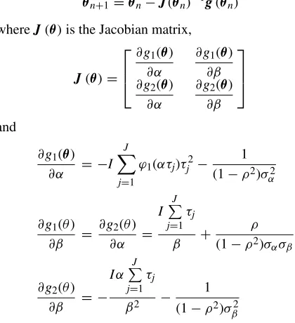
However, since a Gaussian distribution is not a conjugate prior of a Gamma distribution, we cannot achieve a closed form of the mode of the posteriori distribution. As an alter-native, numerical methods, e.g., Newton’s method, can be employed to compute the MAP estimate of θ˜. Letg(θ) = (g1(θ),g2(θ))T, whereg1(θ) =∂h/∂αandg2(θ)=∂h/∂β. Under the framework of Newton’s method, the iteration equa-tion is formulated as
θn+1=θn−J(θn)−1g(θn) (14)
whereJ(θ)is the Jacobian matrix,
J(θ)=
∂g1(θ) ∂α
∂g1(θ) ∂β ∂g2(θ)
∂α
∂g2(θ) ∂β
and
∂g1(θ) ∂α = −I
J X
j=1
ϕ1(ατj)τj2−
1 (1−ρ2)σ2
α
∂g1(θ) ∂β =
∂g2(θ) ∂α =
I J P
j=1 τj
β +
ρ (1−ρ2)σασβ
∂g2(θ) ∂β = −
Iα J P
j=1 τj
β2 − 1
(1−ρ2)σ2
β
V. APPLICATION IN LOCOMOTIVE WHEEL-SETS
[image:6.576.35.280.61.230.2]A case study on the wheel-sets of a heavy haul locomotive is employed to illustrate the proposed maintenance strategy. During operation, the locomotive wheel-sets may suffer an anomaly and are sent to the maintenance station for reprofil-ing. The anomaly includes increased roughness, asymmetry of wheel-sets and so on. Reprofiling can restore the wheels to the normal state but will reduce the wheel diameter, which is used as the degradation index. There are multiple indexes to measure the degradation level of wheel-sets, but the diameter is most commonly used. Therefore, we use wheel diameter as the degradation indicator and develop maintenance strategies accordingly. Fig. 3 shows the process of reprofiling.
[image:6.576.326.508.63.200.2]FIGURE 3. Reprofiling process.
TABLE 1.Measurements of wheel diameters of bogie 195904.
Two bogies, coded as 195904 and 195905, are employed to illustrate the maintenance strategy. Each bogie consists of six wheel-sets; their diameters are presented in Table 1 and Table 2. The tables show the variation of the wheel diameters before and after reprofiling in terms of the running distance. The data used for illustration were provided by a Swedish company, which were collected in a maintenance station where the wheel-sets were being inspected.
Over the life cycle of the wheels, natural wear and reprofiling contribute to the decrease of the wheel diameter [36], [37]. Natural wear occurs when the wheels are in operation and is modeled as a Gamma degradation process in this paper. Various factors contribute to natural wear, including weather, smoothness of the tracks, running speed and cracks. From Table 1 and Table II, we can find that the natural wear is actually the difference between the diameter after reprofiling and the diameter at the next inspection. For illustration, Fig. 4 presents the variation of natural wear with respect to the running distance of bogie 195904. Note that in the current example, the degradation level refers to the diameter of a wheel, and the operation time denotes the running distance. In the subsequent analysis, the data in Table 1 will be used to estimate the prior distribution and the data in Table 2 will serve for estimation of the MAP and update of the degradation parameters.
A. MAINTENANCE UNDER FIXED DEGRADATION PARAMETERS
[image:6.576.39.249.341.571.2]TABLE 2. Measurements of wheel diameters of bogie 195905.
FIGURE 4. Plot of natural wear.
estimation (MLE). From the data in Table 1, the scale parame-ter and the shape parameparame-ter are estimated asαˆ =0.0592,βˆ= 0.4419, and the associated covariance matrix is obtained as
ˆ
6=[I(θ)]−1=
2.6 20 20 172
×10−4
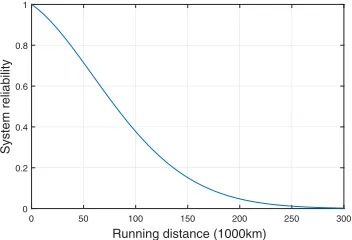
[image:7.576.69.245.547.667.2]For simplicity, the age-dependent failure rate is assumed as constant, λ1(t) = λ0, whereλ0 = 0.0005. The scaling parameter on the degradation level is set asγ =0.001. With the abovementioned parameters, we present the variations in system reliability in Fig. 5.
FIGURE 5. Variations of system reliability.
For a perfect wheel, the initial diameter is 1250mm, and replacement is implemented on the wheel when the diameter tails off to below 1150mm. In this case, the threshold for
replacement is set as ζ = 100mm. The tolerance level is given asη=0.95 for the purposes of illustration. However, in Table 1, we can find that the initial diameter does not exactly match 1250mm; it averages at 1247mm. The differ-ence between the ideal and the measured diameter is due to an error of production and measurement. Thus, the initial degradation level is set asx0=3. It is assumed that the degra-dation increment caused by reprofiling follows a Gaussian distribution, with the parameters estimated as µˆ = 11.87 andσˆ =4.667. From Equation (5), we get the threshold for replacement, and the decision at inspection is given as
πi= (
0, ifxi−≥80.45
1, otherwise
While the wheel is sent to the maintenance station for reprofiling, one has to determine the next inspection time in addition to the maintenance actions. According to Equation (6), Fig. 6 presents the variation of the cost rate in terms of the inspection timeti; in the figure, the
maintenance-related cost is set asci = 10, cp = 70, cc = 100, and cd = 10. The optimal inspection time is obtained atti∗ =
49.8, and the minimal cost rate is given asCR∗ =3.05. The result implies that the optimal running distance is 49,800km given the wheel diameter at 1247mm. In current practice, the optimal inspection time is advised by the manufacturers, but this strategy fails to capture the heterogeneity of the operating environment and the initial diameter of wheel-sets. In current maintenance practice, it is suggested by the manu-facturer that the average running distance between reprofiling should be 40,000km regardless of the heterogeneity in wheel conditions. However, our model suggests that maintenance engineers should dynamically inspect the wheel-sets based upon the present health condition, rather than a fixed value.
FIGURE 6. Cost ratevsinspection time.
FIGURE 7. t∗ i andCR
∗vsdegradation level after reprofiling.
[image:8.576.69.243.230.361.2]due to the fact that an increasedxi+makes the system more prone to failure.
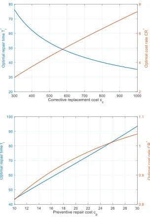
FIGURE 8. Sensitivity analysis oncd,ci,cp,cc.
Sensitivity analysis is conducted to investigate the effect of cost parameters on the optimal inspection time,ti∗, and the associated cost rate,CR∗. Fig. 8 presents the results. As can be observed,CR∗always increases with cost. This is intuitive, since a high cost item lead to a higher cost rate. In addition,
ti∗ shows a decreasing trend with the downtime cost, cd,
and the corrective repair cost, cc, and an increasing trend
FIGURE 9. Histogram oft∗ i andCR
∗, and associated fitted normal pdf
curves.
with the preventive repair cost,cp and the inspection cost,
ci. The system is less likely to fail under higher downtime and corrective repair costs, as this leads to a conservative strategy, i.e., a shorter inspection interval. In contrast, for a highciandcp, maintenance actions are postponed to reduce
the frequency of inspection and the likelihood of preventive repair.
Next, we investigate the influence of parameter estima-tion uncertainty on the optimal maintenance decision. The maximum likelihood estimator asymptotically follows a mul-tivariate normal distribution, θˆ ∼ Nθ,[I(θ)]−1, as θˆ will converge to θ with increased sample size. Therefore,
we employN
ˆ
θ,hI(θˆ)i −1
to approximate the parameter
distribution under large sample sizes. Samples that character-ize the uncertainty of MLE can be obtained by drawing from
the distribution N
ˆ
θ,hI(θˆ)i −1
. Using this distribution
generates 1000 samples, with an optimal inspection timeti∗
and an associated expected cost rateCR∗ for each sample. Fig. 9 plots the histogram ofti∗andCR∗and the associated fitted normal pdf curves. The mean ofti∗is achieved as 49.76, and the standard deviation is 1.3907. ForCR∗, the mean and standard deviation are obtained as 3.06 and 0.0679. The small standard deviation ofti∗andCR∗indicates the effectiveness of MLE.
B. MAINTENANCE WITH UPDATED PARAMETERS
[image:8.576.43.271.445.617.2]TABLE 3. Update of parameters at inspections.
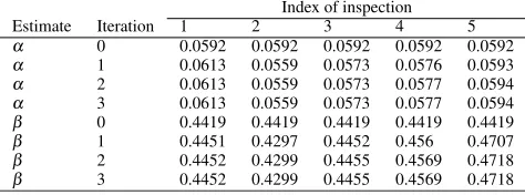
TABLE 4. Iteration of Newton’s method for the sixth wheel-set.
we update the six wheel-sets of Table 2 separately; i.e., the distribution parameters of each wheel-set are estimated only by the prior information and the associated observations. With the MAP procedure presented in Section IV, we can compute the updated parameters, as shown in Table 3. Unlike the estimates using MLE, the estimates using MAP vary for different wheel-sets, thus describing the heterogeneity of the wheel-sets. In addition, variations of θ at each inspection indicate the flexibility and power of incorporating the new information.
Since the Gaussian distribution is not a conjugate prior, a closed-form solution of Equation (12) cannot be achieved. Therefore, we use Newton’s method to compute the estimates from MAP. The initial guess of Newton’s method is identical to the prior distribution, θ0 = (0.0592,0.4419). Following the iteration procedure in Equation (14), we can obtain the updated parameters given the observed data at each inspec-tion. Taking the sixth wheel-set for example,Table 4 presents the variation of the parameters at each iteration. It can be observed that the estimates converge quickly, mostly in two iterations, indicating that the updated estimates are closed to the initial guess. At each inspection, given the current degradation level and the updated parameters, the optimal subsequent inspection time can be achieved by minimizing the average cost rate in Equation (6).
C. COMPARISON WITH CONTINUOUS MONITORING This section presents a case where the degradation level of the system can be continuously monitored. Compared with the discrete inspection in Section III, under continuous
monitoring, repair or replacement is carried out immediately if the system is found to have failed. Therefore, no downtime is considered in this scenario. In addition, the inspection cost is suppressed since the system is under continuous monitor-ing. The maintenance strategy under continuous monitoring works as follows: given the degradation level after repairxi+, the system is repaired preventively at timeTior correctively
at failureTf. The corresponding cost rate is given as
CR Ti;xi+= cp
+ cc−cp 1− ¯R(Ti;xi+)
Emin{Ti,Tf}
(15)
where the expected cycle lengthE
min{Ti,Tf}is given as
Emin{Ti,Tf}=E Z Ti
0
1−F(t|XTi 0)
dt|XTi
0
Upon repair, the system age is reduced to 0, while the degradation level increases. In other words, after repair or replacement, the system age is reduced to 0. Therefore, in the subsequent repair cycle, the system age will always start from 0. In Equation (15), the reliability function performs differ-ently in terms of the repair or replacement (the degradation levelxi+differs).
For a degradation process with small variance,
Emin{Ti,Tf}
can be approximated as Emin{Ti,Tf}
≈
RTi 0 R¯(t;x
+
i )dt. [38] states that the optimal maintenance
strat-egy for the above problem is a control limit stratstrat-egy, with the optimal repair time expressed as
Ti∗=inf
t≥0, λ t,X(t);xi+≥CR∗/ cc/cp−1
Since the optimal expected one-cycle cost rate is depen-dent on the associated repair time,Ti∗, an iterative algorithm is proposed for computation purposes [38], [39]. Although the iterative algorithm works well for a deterministic or discrete degradation process, it cannot be applied for a continuous degradation process, as the hazard rate func-tion λ t,X(t);xi+ is randomized by X(t). Therefore, we resort to a one-directional search algorithm to obtain the optimal repair time, Ti∗. In fact, Equation (15) can be rewritten as
CR Ti;x+
i
=
cp1
+(K−1) 1− ¯R(Ti;xi+)
Emin{Ti,Tf}
[image:9.576.38.275.249.337.2]FIGURE 10. Influence ofccandcpunder continuous monitoring.
continuous monitoring. The variation trend of Ti∗ andCR∗
is similar to that found in discrete inspection.
VI. CONCLUSION
This paper presents a dynamic maintenance strategy for sys-tems subject to aging and degradation. During operation, the system goes through an aging and degradation process, which affects the failure rate of the system in an additive way. System reliability is analyzed as a first step, followed by a maintenance model evaluated based on the expected cost rate within a repair cycle. A dynamic maintenance strategy is proposed, where the degradation parameters are updated and the optimal subsequent inspection time is provided at each maintenance action. The proposed maintenance model has two advantages compared with the existant time-based pre-ventive maintenance models. First, it incorporates the effects of both the aging and degradation. Second, it permits decision makers to dynamically determine the optimal inspection time and the associated maintenance actions based on the observed degradation level and the operating history, thereby adapting to heterogeneous operating conditions. Application of the model to a case study of locomotive wheel-sets shows its effectiveness.
Future research can take two directions. First, it is assumed in this study that the degradation level of the system can be perfectly inspected, but in reality, observations are usu-ally contaminated by noise. In future research, filtering approaches, such as the Kalman filter and its variants, and particle filters, can be employed to estimate the degradation level and the parameters of interest. Second, the optimal maintenance strategy is achieved based on the criterion of the average cost rate. However, if the cost parameters are sub-ject to high uncertainty, i.e., cost items cannot be accurately evaluated, criteria that are independent of the cost parameters,
such as availability, reliability, and remaining useful lifetime, could be applied.
APPENDIX
A. PROOF OF PROPOSITION 1
Consider the degradation-dependent failure rate λ2(X(t)). Based on the scaling property of the Gamma process, it fol-lows thatλ2(X(t)) =γX(t) ∼Ga(t;α, β/γ )The Gamma process belongs to the class of L´evy processes, where the Levy measure of´ λ2(X(t))is given as
v(dy)=y−1αexp(−βy/γ)dy
The theorem (Corollary 3.3) of [31] indicates that a reliability function with an increasing L´evy failure rate process can be transformed to one with a deterministic failure rate,
h(t)=
Z ∞
0
1−exp(−tx)v(dx)
Then it follows that,
E
exp
−
Z t
0
λ2(X(s))ds
=exp
−γx0t−
Z t
0
ds
Z ∞
0
αexp(−βy/γ)y−1
·(1−exp(−(t−s)y)dy)
=exp
−γx0t−
Z t
0 αlog
β/γ+t−s
β/γ
ds
=exp
−γx0t−
Z t
0 αlog
β/γ+s
β/γ
ds
Combined with the additive model of Equation (4), system reliability is provided as
¯
R(t)=E
exp
−
Z t
0
λ1(s)+λ2(X(s))ds
=exp
−
Z t
0
λ1(s)ds
·E
exp
−
Z t
0
λ2(X(s))ds
=exp
−
Z t
0
λ1(s)+γx0t+αlog
β+γs
β
ds
which completes the proof.
B. DERIVATION OF EQUATION (7)
LetTs be the smaller of the inspection time and the time to
failure,Ts =min
ti,Tf . It follows that
E[Ts]=ti 1−EF(ti|X0ti)|X0ti
+E Z ti
0
tdF(t|Xti 0)|X
ti 0
=E Z ti
0
1−F(t|Xti 0)
dt|Xti
0
Since downtime only occurs when the system fails before inspection/repair, we have
Td=max
By definition, Td can be rewritten as Td = ti −Ts. Its expectation is readily obtained as
E[Td]=tiF(ti)−
Z ti
0
tdF(t)
=E Z ti
0
F(t|Xti 0)dt|X
ti 0
=E Z ti
0
1−exp
−
Z t
0 λ (
s,X(s))ds
dt|Xti 0
C. PROOF OF COROLLARY 2
Denote the expected cost in a repair cycle as
CT(ti;xi+)=ci+cp+ cc−cp
1− ¯R(ti;xi+)
+cd Z ti
0
1− ¯R(ti;xi+)
Obviously,CT(ti;xi+)>0 forti ∈ (0,∞). By taking the
derivative of the expected average cost in Equation (10) with respect toti, we have
CR0 ti;xi+= tiCT
0(ti;x+
i )−CT(ti;x + i ) ti2
Whentiapproaches zero from the right,ti→0+, we clearly
have lim
ti→0
CR0 ti;xi+
< 0. When ti approaches infinity,
it follows
lim
ti→∞
tiCT0(ti)−CT(ti)
= lim
ti→∞
cd
ti 1− ¯R(ti;xi+)
−
Z ti
0
1− ¯R(ti;xi+)
−ci−cc
=cdν−ci−cc
Ifν >(ci+cc)/cd, we have lim ti→∞
CR0 ti;xi+>0, which
completes the proof.
D. ESTIMATION OF THE PRIOR DISTRIBUTION
DenoteN as the number of units andM the number of time records of the historical data. Denoteτ¯jas thejth time record,
j =1,2. . . .,M, andxij¯ as the degradation increment of the
ith unit in time intervalτ¯j,i = 1,2, . . . ,N. The likelihood function is expressed as
L(α, β)=
N Y
i=1
M Y
j=1
f(x¯ij|α, β)
=
N Y
i=1
M Y
j=1 βατ¯j 0 ατ¯j
¯
xijατ¯j−1e−βx¯ij
and the log-likelihood function is given as
l(α, β)=N M X
j=1
ατ¯jln(β)+
N X
i=1
M X
j=1
(ατ¯j−1) ln(x¯ij)
−β
N X
i=1
M X
j=1 ¯
xij−N M X
j=1
ln 0(αtj) (A1)
Let the derivative ofβbe 0,
∂l
∂β =
Nα M P
j=1 ¯ τj
β −
N X
i=1
M X
j=1 ¯
xij=0
It follows that
ˆ β =
Nα M P
j=1 ¯ τj
N P
i=1
M P
j=1 ¯
xij
(A2)
Taking the derivative ofαleads to
∂l
∂α =Nln(β)
M X
j=1 ¯ τj+
N X
i=1
M X
j=1 ¯
τjln(xij¯ )−N M X
j=1
ϕ(ατ¯j)τ¯j
(A3)
whereϕ(·) is the digamma function,
ϕ(z)= 0
0(z)
0(z)
Substituting Equation (A2) into Equation (A3), and letting the derivative be zero leads to
N M X
j=1
ϕ(ατ¯j)τ¯j−Nln(α)
M X
j=1 ¯ τj =N ln N M X
j=1 ¯ τj M X
j=1 ¯ τj−Nln
N X
i=1
M X
j=1 ¯ xij M X
j=1 ¯ τj
+
N X
i=1
M X
j=1 ¯
τjln(x¯ij) (A4)
Equation (A4) can be solved via numerical methods, e.g., Newton’s method. Based on the estimatedαˆ, the estimate ofβcan be readily obtained from Equation (A2).
The Fisher information matrix is obtained by taking the second derivation ofαandβ. It follows that
I(θ)=
N M X
j=1
ϕ1(ατ¯j)τ¯j2 −
N M P
j=1 ¯ τj β − N M P
j=1 ¯ τj β Nα M P
j=1 ¯ τj β2
whereϕ1(·) is the trigamma function,
ϕ1(z)= dϕ(z)
dz
NOTATION
X(t) Degradation level at timet
Ga(t;α, β) Gamma process with shape parameterαand scale parameterβ
1X(t−l) Degradation increment between timetandl
λ(t,X(t)) System failure rate ¯
R(t) Expected system reliability at timet
λ1(t) Age-related failure rate
λ2(X(t)) Degradation-dependent failure rate
Tf Time to failure
Xi− Degradation level before theith repair
Xi+ Degradation level after theith repair
Yi Degradation increment at theith repair
π ∈ {0,1} Maintenance decision: replacement (πi=0)
or repair (πi=1)
ζ Threshold for replacement
η Tolerance level of degradation after repair
ti Time interval between theith and (i+1)th inspection
CR Long-run cost rate
ci,cp,cc Cost of inspection, preventive repair
and corrective replacement
cd Downtime cost per unit time
Td Downtime
θ=(α, β)T Set of degradation parameters
p(θ) pdf of prior distribution
f(θ|x) Posteriori distribution ofθgiven the datasetx I(θ) Fisher information evaluated atθ
ˆ
θ MLE estimate ofθ ˜
θ MAP estimate ofθ
L(θ) Likelihood function
REFERENCES
[1] R. Karim, J. Westerberg, D. Galar, and U. Kumar, ‘‘Maintenance analytics—The new know in maintenance,’’IFAC-PapersOnLine, vol. 49, no. 28, pp. 214–219, 2016.
[2] K. Matyas, T. Nemeth, K. Kovacs, and R. Glawar, ‘‘A procedural approach for realizing prescriptive maintenance planning in manufacturing indus-tries,’’CIRP Ann., vol. 66, no. 1, pp. 461–464, 2017.
[3] S. Alaswad and Y. Xiang, ‘‘A review on condition-based maintenance optimization models for stochastically deteriorating system,’’Rel. Eng. Syst. Saf., vol. 157, pp. 54–63, Jan. 2017.
[4] M. Compare, F. Martini, S. Mattafirri, F. Carlevaro, and E. Zio, ‘‘Semi-Markov model for the oxidation degradation mechanism in gas turbine nozzles,’’IEEE Trans. Rel., vol. 65, no. 2, pp. 574–581, Feb. 2016. [5] Z. Liang and A. K. Parlikad, ‘‘A condition-based maintenance model for
assets with accelerated deterioration due to fault propagation,’’IEEE Trans. Rel., vol. 64, no. 3, pp. 972–982, Jun. 2015.
[6] H. Dui, S. Si, M. J. Zuo, and S. Sun, ‘‘Semi-Markov process-based integrated importance measure for multi-state systems,’’IEEE Trans. Rel., vol. 64, no. 2, pp. 754–765, Apr. 2015.
[7] M. Zhang and M. Revie, ‘‘Continuous-observation partially observable semi-Markov decision processes for machine maintenance,’’IEEE Trans. Rel., vol. 66, no. 1, pp. 202–218, Mar. 2017.
[8] Z.-S. Ye and M. Xie, ‘‘Stochastic modelling and analysis of degradation for highly reliable products,’’Appl. Stochastic Models Bus. Ind., vol. 31, no. 1, pp. 16–32, 2015.
[9] B. de Jonge, R. Teunter, and T. Tinga, ‘‘The influence of practical factors on the benefits of condition-based maintenance over time-based mainte-nance,’’Rel. Eng. Syst. Saf., vol. 158, pp. 21–30, Feb. 2017.
[10] X. Zhao, O. Gaudoin, L. Doyen, and M. Xie, ‘‘Optimal inspection and replacement policy based on experimental degradation data with covari-ates,’’IISE Trans., vol. 51, no. 3, pp. 322–336, 2019.
[11] B. Liu, S. Wu, M. Xie, and W. Kuo, ‘‘A condition-based maintenance policy for degrading systems with age- and state-dependent operating cost,’’Eur. J. Oper. Res., vol. 263, no. 3, pp. 879–887, 2017.
[12] B. Liu, R.-H. Yeh, M. Xie, and W. Kuo, ‘‘Maintenance scheduling for multicomponent systems with hidden failures,’’IEEE Trans. Rel., vol. 66, no. 4, pp. 1280–1292, Dec. 2017.
[13] Q. Zhai and Z.-S. Ye, ‘‘Degradation in common dynamic environments,’’
Technometrics, vol. 60, no. 4, pp. 461–471, 2018.
[14] X. Zhao, J. Xu, and B. Liu, ‘‘Accelerated degradation tests planning with competing failure modes,’’IEEE Trans. Rel., vol. 67, no. 1, pp. 142–155, Oct. 2018.
[15] P. Do, A. Voisin, E. Levrat, and B. Iung, ‘‘A proactive condition-based maintenance strategy with both perfect and imperfect maintenance actions,’’Rel. Eng. Syst. Saf., vol. 133, pp. 22–32, Jan. 2015.
[16] P. Chen and Z.-S. Ye, ‘‘Random effects models for aggregate lifetime data,’’
IEEE Trans. Rel., vol. 66, no. 1, pp. 76–83, Mar. 2017.
[17] Z.-S. Ye and N. Chen, ‘‘The inverse Gaussian process as a degradation model,’’Technometrics, vol. 56, no. 3, pp. 302–311, Jul. 2014.
[18] J. M. Van Noortwijk, ‘‘A survey of the application of gamma processes in maintenance,’’Rel. Eng. Syst. Saf., vol. 94, no. 1, pp. 2–21, Jan. 2009. [19] B. Cai, X. Kong, Y. Liu, J. Lin, X. Yuan, H. Xu, and R. Ji, ‘‘Application of
Bayesian networks in reliability evaluation,’’IEEE Trans. Ind. Informat., vol. 15, no. 4, pp. 2146–2157, Jul. 2019.
[20] K. Rafiee, Q. Feng, and D. W. Coit, ‘‘Reliability modeling for dependent competing failure processes with changing degradation rate,’’IIE Trans., vol. 46, no. 5, pp. 483–496, 2014.
[21] S. Song, D. W. Coit, and Q. Feng, ‘‘Reliability analysis of multiple-component series systems subject to hard and soft failures with dependent shock effects,’’IIE Trans., vol. 48, no. 8, pp. 720–735, 2016.
[22] J. H. Cha, M. Finkelstein, and G. Levitin, ‘‘Bivariate preventive mainte-nance of systems with lifetimes dependent on a random shock process,’’
Eur. J. Oper. Res., vol. 266, no. 1, pp. 122–134, 2018.
[23] L. Yang, Y. Zhao, R. Peng, and X. Ma, ‘‘Hybrid preventive maintenance of competing failures under random environment,’’Rel. Eng. Syst. Saf., vol. 174, pp. 130–140, Jun. 2018.
[24] C. Zhang, H. Wu, R. Bie, R. Mehmood, and A. Kos, ‘‘Dynamic modeling of failure events in preventative pipe maintenance,’’IEEE Access, vol. 6, pp. 12539–12550, 2018.
[25] J. Lin, M. Asplund, and A. Parida, ‘‘Reliability analysis for degradation of locomotive wheels using parametric Bayesian approach,’’Qual. Rel. Eng. Int., vol. 30, no. 5, pp. 657–667, 2014.
[26] J. Lin, J. Pulido, and M. Asplund, ‘‘Reliability analysis for preventive maintenance based on classical and Bayesian semi-parametric degradation approaches using locomotive wheel-sets as a case study,’’Rel. Eng. Syst. Saf., vol. 134, pp. 143–156, Feb. 2015.
[27] K. Rafiee, Q. Feng, and D. W. Coit, ‘‘Reliability analysis and condition-based maintenance for failure processes with degradation-dependent hard failure threshold,’’Qual. Rel. Eng. Int., vol. 33, no. 7, pp. 1351–1366, 2017. [28] X. Liu, J. Li, K. N. Al-Khalifa, A. S. Hamouda, D. W. Coit, and E. A. Elsayed, ‘‘Condition-based maintenance for continuously monitored degrading systems with multiple failure modes,’’IIE Trans., vol. 45, no. 4, pp. 422–435, 2013.
[29] A. Lehmann, ‘‘Joint modeling of degradation and failure time data,’’J. Stat. Planning Inference, vol. 139, no. 5, pp. 1693–1706, 2009.
[30] B. Liu, Z. Liang, A. K. Parlikad, M. Xie, and W. Kuo, ‘‘Condition-based maintenance for systems with aging and cumulative damage based on proportional hazards model,’’Rel. Eng. Syst. Saf., vol. 168, pp. 200–209, Dec. 2017.
[31] Y. Kebir, ‘‘On hazard rate processes,’’Nav. Res. Logistics, vol. 38, no. 6, pp. 865–876, 1991.
[32] T. Nakagawa, ‘‘Sequential imperfect preventive maintenance policies,’’
IEEE Trans. Rel., vol. R-37, no. 3, pp. 295–298, Aug. 1988.
[33] S. H. Sheu and C. C. Chang, ‘‘An extended periodic imperfect preventive maintenance model with age-dependent failure type,’’IEEE Trans. Rel., vol. 58, no. 2, pp. 397–405, Jun. 2009.
[35] X. Zhu, X. Bei, N. Chatwattanasiri, and D. W. Coit, ‘‘Optimal system design and sequential preventive maintenance under uncertain aperiodic-changing stresses,’’ IEEE Trans. Rel., vol. 67, no. 3, pp. 907–919, Feb. 2018.
[36] J. Lin and M. AspLund, ‘‘Comparison study of heavy haul locomotive wheels’ running surfaces wearing,’’Eksploatacja Niezawodnosc, vol. 16, no. 2, pp. 276–287, 2014.
[37] B. Liu, J. Lin, L. Zhang, and M. Xie, ‘‘A dynamic maintenance strategy for prognostics and health management of degrading systems: Application in locomotive wheel-sets,’’ inProc. IEEE Int. Conf. Prognostics Health Manage. (ICPHM), Jun. 2018, pp. 1–5.
[38] B. Bergman, ‘‘Optimal replacement under a general failure model,’’Adv. Appl. Probab., vol. 10, no. 2, pp. 431–451, 1978.
[39] X. Wu and S. M. Ryan, ‘‘Optimal replacement in the proportional hazards model with semi-Markovian covariate process and continuous monitor-ing,’’IEEE Trans. Rel., vol. 60, no. 3, pp. 580–589, Jul. 2011.
BIN LIUreceived the B.S. degree in automation from Zhejiang University, China, and the Ph.D. degree in industrial engineering from the City University of Hong Kong, Hong Kong. He was a Postdoctoral Fellow with the University of Waterloo, Canada. He is currently a Lecturer with the Department of Management Science, Univer-sity of Strathclyde, Glasgow, U.K. His research interests include risk analysis, reliability and maintenance modeling, decision making under uncertainty, and data analysis.
JING (JANET) LINreceived the Ph.D. degree in management from the Nanjing University of Sci-ence and Technology, in 2008. She is currently an Associate Professor with the Division of Operation and Maintenance Engineering, Luleå University of Technology (LTU), Luleå, Sweden. She is also a joint Professor with Beijing Jiaotong Univer-sity, Beijing, China. Her research interests include Bayesian reliability modeling, maintenance engi-neering, and prognostics and health management.
LIANGWEI ZHANGreceived the Ph.D. degree in operation and maintenance engineering from the Luleå University of Technology, Luleå, Sweden, in 2017. From 2009 to 2013, he was a Consul-tant of reliability engineering with SKF, Beijing, China. He is currently a Lecturer with the Depart-ment of Industrial Engineering, Dongguan Univer-sity of Technology, Dongguan, China. He is also an Adjunct Lecturer with the Division of Operation and Maintenance Engineering, Luleå University of Technology. His research interests include machine learning, fault detection, and prognostics and health management.