Co Synthesis of Energy Efficient Multi Mode Embedded Systems with Consideration of Mode Execution Probabilities

Co-Synthesis of Energy-Efficient Multi-Mode Embedded Systems

with Consideration of Mode Execution Probabilities

Marcus T. Schmitz1,2, Bashir M. Al-Hashimi1, Petru Eles2 1_{Electronic Systems Design Group}

Department of Electronics and Computer Science University of Southampton, Southampton, UK

[email protected]

2_{Department of Computer and Information Science} Linköping University

S-581 83 Linköping, Sweden {g-marsc, petel}@ida.liu.se

Final version: 19 March 2004

Abstract

In this paper, we present a novel co-design methodology for the synthesis of energy-efficient embedded systems. In particular we concentrate on distributed

em-bedded systems that accommodate several different applications within a single de-vice, i.e., multi-mode embedded systems. Based on the key observation that

opera-tional modes are executed with different probabilities, i.e., the system spends uneven amounts of time in the different modes, we develop a new co-design technique that

exploits this property to significantly reduce energy dissipation. The energy savings

are achieved through a suitable synthesis process that yields better hardware resource sharing opportunities for both cost and energy reduction. We conduct several

exper-iments, including a realistic smart phone example that demonstrate the effectiveness of our approach. Reductions in power consumption of up to 64% are reported.

1

Introduction

Over the last several years, the popularity of portable applications has explosively increased.

Mil-lions of people use battery-powered mobile phones, digital cameras, MP3 players, and personal

digital assistants (PDAs). To perform major parts of the system’s functionality, these mass

prod-ucts rely, to a great extent, on sophisticated embedded computing systems with high performance

and low power dissipation. One key characteristic of many current and emerging embedded

For instance, modern mobile phones often integrate not solely the functionality required for

com-munication purpose (e.g., voice coding and protocol handling), but additionally integrate

appli-cations like digital cameras, games, and complex multimedia functions (MP3 players and video

decoders) into the same single device. Throughout this article, such embedded systems are referred

to as multi-mode embedded systems. This paper introduces a novel co-synthesis methodology

par-ticular suitable for the design of energy-efficient multi-mode embedded systems. Starting from

a specification model that captures both mode interaction and functionality, the developed

co-synthesis technique maps the application under consideration of mode execution probabilities to

a heterogeneous, distributed architecture with the aim to reduce the energy consumption through

an appropriate resource sharing between tasks. Mode execution probabilities refer to the

activa-tion time of operaactiva-tional modes that are user typical. Consider for instance the typical activaactiva-tion

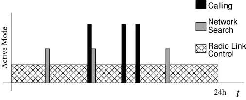
Calling Network Search Control Radio Link

t

Figure 1: Typical Activation Profile of a Mobile Phone

profile of a mobile phone, which is shown in Figure 1. According to this profile, the phone stays

most of the time in aRadio Link Controlmode, in order to maintain network connectivity. While

theNetwork Search mode and theCalling mode are only active for small periods of the overall

time. The main principle by which the proposed co-synthesis process achieves energy-efficiency

is an implementation trade-off between the different operational modes. In general, modes with

high execution probability should be implemented more energy efficient (e.g., by moving more

tasks to hardware) than modes with a low execution probability. Nonetheless, the implementation

of modes is heavily interrelated, due to the fact that different modes share the same resources

(architecture). For example, mapping an critical task of a highly active mode into

energy-efficient hardware might prohibit to implement a timing-critical task into hardware due to the

restricted hardware area (see motivational example in Section 4). Clearly, a well balanced

imple-mentation of the operational modes is vital for a good system design. In addition, the co-synthesis

approach further reduces the energy dissipation by adapting the system performance to the

par-ticular needs of the active mode, using dynamic voltage scaling (DVS) as well as component

shutdown. That is, instead of wasting energy through over-performance, the computational power

is adapted according to the individual performance requirements of each mode and each task.

order to allow the scaling of hardware processing elements that are capable of executing tasks in

parallel, however, which rely on a single scalable supply voltage source.

The remainder of this paper is organized as follows. Section 2 introduces relevant previous

work. Preliminaries, outlining a new multi-mode specification and an architectural model, are

given in Section 3. Motivational examples exemplify the need for a suitable multi-mode synthesis

approach in Section 4. The problem at hand is formulated in Section 5. Section 6 describes

our multi-mode co-synthesis approach, and Section 7 presents experimental results. Finally, in

Section 8 we draw some conclusions.

2

Previous Work

In the last decade, numerous methodologies for the design of low power consuming embedded

systems have been proposed, including approaches that leverage power management techniques,

such as dynamic power management (DPM) and dynamic voltage scaling (DVS). Nevertheless, a

crucial feature of many modern embedded systems is their capability to execute several different

applications (multi-modes), which are integrated into a single device.

Approaches for the schedulability analysis of systems with several modes of operations can be

found in the real-time research community [31, 26]. However, these approaches solely concentrate

on scheduling aspects (i.e., they investigate if the mode change events fulfil the imposed timing

constraints) and do not address implementation aspects. Three recent approaches have addressed

various problems involved in the design of multi-mode embedded systems [21, 25, 32]. Shin et al.

[32] proposed a schedulability-driven performance analysis technique for real-time multi-mode

systems. They show that it is possible, through a sophisticated performance estimation, to identify

timing-critical tasks, which are active in different operational modes. This identification allows to

improve the execution times of the most crucial tasks, in order to achieve system schedulabilitly.

In their work, the optimization of the identified tasks is up to the designer. For example, reductions

in the execution times can be made by handcrafted code tuning and outsourcing of core routines

into hardware. Kalavade and Subrahmanyam [21] have introduced a hardware/software

partition-ing approach for systems that perform multiple functions. Their technique classifies tasks, found

within similar applications, into groups of task types. The implementation of frequently

appear-ing task types is biased towards hardware. This can be intuitively justified by the fact that costly

hardware implementations are shared across a set of applications, hence, exploiting the allocated

hardware more cost effective. Oh and Ha [25] address the problem in a slightly different way.

Their co-synthesis framework for multi-mode systems is based on a combined scheduling and

mapping technique for heterogeneous multiprocessor systems (HMP [24]). Taking a processor

(PEs) such that the schedulability constraint is satisfied and the system cost is minimized. The

main principle behind all three approaches is to consider the possibility of resource sharing, i.e.,

computational tasks of the same type, which can be found in different modes, utilize the same

implementations. Thereby, multiple hardware implementations of the same task type are avoided,

which, in turn, reduces the hardware cost. Other noticeable approaches are the works by Chung

et al. [11] and Yang et al. [34]. In [11], energy efficiency is achieved by leveraging information

regarding the execution time variations, which is supplied to the mobile terminal by the contents

provider. That is, the performance of the mobile terminal can be influenced directly by the

con-tents provider, in accordance to the processing requirements of the sent content. The approach

presented in [34] uses a two-phase scheduling method. In the first stage, which is performed

off-line (during design time), a Pareto-optimal set of schedules is generated. These schedule provide

different execution time/energy trade-offs. During run-time, a run-time scheduler selects points

along the Pareto set, in order to account for the dynamic behavior of the application. As opposed

to these approaches, the work presented in this paper addresses the design of low energy

consum-ing multi-mode systems that exhibit variations in the mode activation profile; hence, it differs in

several aspects from the previous works. To the authors’ knowledge, there has been no prior work

investigating the co-design problem of energy minimization taking into account mode execution

probabilities. This paper makes the following contributions:

(a) The consideration of mode execution probabilities and their effect on the energy-efficiency

of multi-mode embedded systems is analysed and demonstrated.

(b) A co-design methodology for the design of energy-efficient multi-mode systems is

pre-sented. The proposed co-synthesis maps and schedules a system specification that captures

both mode interaction and mode functionality onto a distributed heterogeneous architecture.

Four mutation strategies are introduced that aid the genetic algorithm-based optimization

process in finding solutions of high quality by pushing the search into promising design

space regions.

(c) Dynamic voltage scaling is investigated in the context of multi-mode embedded systems. A

transformation-based approach is used to tackle the problem of DVS on processing elements

that execute different tasks in parallel, but offer only a single scalable supply voltage source.

3

Preliminaries

This section introduces the functional specification model (Section 3.1) and the architectural model

GSM codec + RLC Ψ1=0.74

Ψ2=0.01

Ψ3=0.02

Ψ4=0.02

Ψ5=0.1

Ψ6=0.01

Ψ7=0.01

Ψ0=0.09

Radio Link Control decode Photo =0.025s HD deQ IDCT Tr. color coeff. 256 256 256 256 RLC =0.015s θ

θ =0.025s

φ

(b) Task Graph of a single Mode

Search

Network Radio_Link Control Take

Photo Photo decode

Search + NeworkPhoto

+ RLC + RLC MP3 play MP3 play + Nework Search Network found Network found Network found Network lost Show

Photo ShowPhoto

Incoming Call User request /

Terminate Call audio Play audio Play Terminate Terminate audio audio

Terminate Terminate_Photo

Photo Photo Photo taken taken Take Photo Take Photo decode INIT

(a) Operational Modes

Network lost

Network lost tmax= 30ms tmax= 30ms

tmax= 30ms

4,7

1,2

5,6

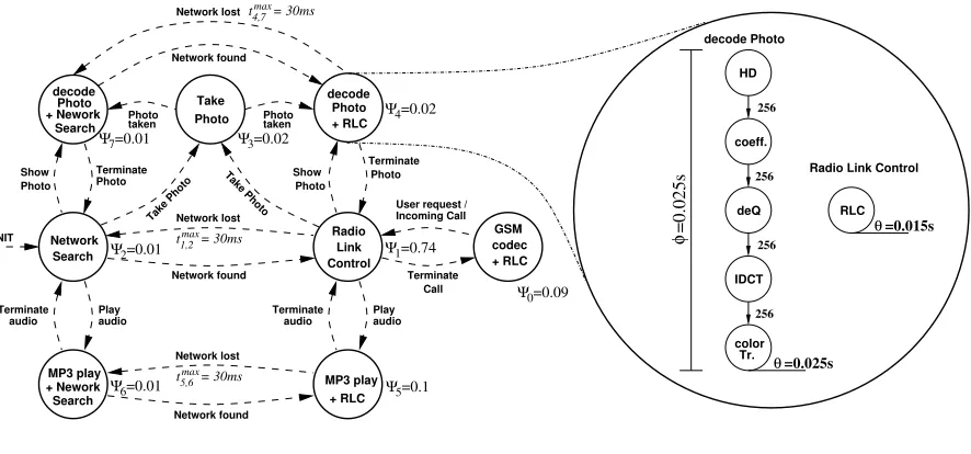
Figure 2: Relation between OMSM and individual task graph specifications

3.1 Functional Specification of Multi-Mode Systems

The abstract specification model used for multi-mode embedded systems consists of two parts.

In précis, it is based on a combination of finite state machines and task graphs, capturing both

the interaction between different operational modes as well as the functionality of each individual

mode. Structurally, each node in the finite state machine represents an operational mode and

further contains the task graphs which are active during this mode. The following two sections

introduce this model, which is henceforth referred to as operational mode state machine (OMSM).

A similar abstract model was mentioned in [17]. However, here this model is extended towards

system-level design and includes transition time limits as well as mode execution probabilities.

The following introduces this model, using the smart phone example shown in Figure 2.

Top-level Finite State Machine

In this work, it is considered that an application is given as a directed cyclic graphϒ(Ω,Θ), which

represents a finite state machine. Within this top-level model, each node O∈Ωrefers to an

op-erational mode and each edge T ∈Θspecifies a possible transition between two different modes.

If the system undergoes a change from mode Ox to mode Oy, where x6=y, the transition time

t_Tmax associated with the transition edge T = (Ox,Oy)has to be met. For instance, as indicated in

Figure 2(a), upon losing the network connection the system needs to activate theNetwork Search

mode within 30ms. Such transition overheads can originate from the reconfiguration of FPGAs

as well as from loading the application software of the particular mode into the local PE memory.

exemplify the proposed model consider Figure 2(a). This figure shows the operational mode state

machine for a smart phone example with eight different modes. A possible activation scenario

could look like this: When switched on, the phone initialises intoNetwork Searchmode. The

sys-tem stays in this mode until a suitable network has been found. Upon finding a network the phone

undergoes a mode change toRadio Link Control (RLC). In this mode it maintains the connection to

the network by handling cell hand-overs, radio link failure responses, and adaptive RF power

con-trol. An incoming phone call necessitates to switch the system intoGSM codec + RLCmode. This

mode is responsible for speech encoding and decoding, while simultaneously maintaining network

connectivity. Similarly, the remaining modes have different functionalities and are activated upon

mode change events. Such events originate upon user requests (e.g. MP3-player activation) or are

initiated by the system itself (e.g. loss of network connection necessitates to switch the system

into network search mode). Furthermore, based on the key observation that many multi-mode

systems spend their operational time unevenly in each of the modes, an execution probabilityΨO

is associated with each operational mode O, i.e., it is known what percentage of the operational

time the device spends in each mode. For instance, in accordance to Figure 2, the smart-phone

stays 74% of this operational time inRadio Link Control (RLC)mode, 9% inGSM codec + RLC

mode, and 1% inNetwork Searchmode. The remaining 16% of the operation time are associated

with the remaining modes. In practice the mode probabilities vary from user to user, depending

on the personal usage behavior. Nevertheless, it is possible to derive an average activation profile

based on statistical information collected from several different users. Taking this information

into account will prove to be important when designing systems with a prolonged battery lifetime.

It is interesting to note that different operational modes do not necessarily correspond to

differ-ent functionalities of the system. For example, alternative modes can be used to model the same

functionality under different working conditions (such as different workloads). For instance, in

order to account for variations in the wireless channel quality, we could exchange the GSM voice

transcoder mode O0in Figure 2(a) with three transcoder schemes, each responsible for the coding

at a different signal-to-interference ratio (SIR) on the channel. During run-time the appropriate

transcoder scheme would be selectively activated, depending on the actual channel quality.

Functional Specification of Individual Modes

The functional specification of each operational mode O∈Ωin the top-level finite state machine

is expressed by a task graph GO_S(

T

C

_T

a task graph represents a task, i.e., a fragment of functionality that needs to be executed without

preemption. The level of granularity is coarse, i.e., tasks refer to functions such as Huffman

de-coder, de-quantizer, FFT, IDCT, etc. Therefore, each task is further associated with a task type

MEM

MEM ASIC

Interface

DVS−Contr.

CPU

Interface

DSP

BUS

SW C1: FFT

C2: HD C3: IDCT C4: Color Trans.

C5: DeQ C6: STP C7: LTP HW

Interface C5

C6 C7

C2

C4

DVS−Contr.

C1

C3 Interface

FPGA Cores

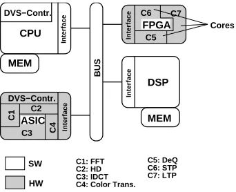
Figure 3: Distributed Architectural Model

setsΓO⊆Γof different modes O∈Ωcan intersect, i.e., tasks of same type are executed in

dif-ferent modes. Such modes can share the same hardware resource (inter-mode sharing). Resource

sharing is also possible for multiple tasks of identical type that are found in a single mode

(intra-mode sharing); however, due to task communalities among different (intra-modes, the chances to share

resources are increased. Further, tasks might be annotated with deadlines θτ (withτ∈

_T

which the execution has to be finished, in order to guarantee correct functioning. Similarly, the

whole task graph has to be successively repeated according to a periodφO. Edgesγ∈

C

graph refer to precedence constraints and data dependencies between the computational tasks, i.e.,

if two tasks,τiandτj, are connected via an edge, then taskτimust be finished and transfer data to

taskτj, beforeτjcan be executed. A feasible implementation of a certain mode O needs to respect

all task deadlinesθ, task graph periodφ, and precedence relations.

3.2 Architectural Model and System Implementation

The proposed system-level synthesis approach targets distributed architectures that possibly

con-sist of several heterogeneous processing elements (PEs), such as general-purpose processors (GPPs),

application-specific instruction set processors (ASIPs), ASICs, and FPGAs. These components are

connected through an infrastructure of communication links (CLs). A directed graph GA(

P

L

captures such an architecture, where nodesπ∈

_P

_L

respec-tively. Figure 3 shows an architecture example. Since each task might have multiple

implemen-tation alternatives, it can be potentially mapped onto several different PEs that are capable of

performing this type of task. Tasks mapped to software-programmable components (i.e., GPP or

ASIP) are placed into local memory. However, if a task is mapped to a hardware component (i.e.,

ASIC or FPGA), a core for this task type needs to be allocated. A feasible solution needs to obey

the imposed area constraints, i.e., only a restricted number of cores can be implemented on

hard-ware components. The subdivision of hardhard-ware components (ASICs and FPGAs) into hardhard-ware

time. Tasks assigned to GPPs or ASIPs (software tasks) need to be sequenced, whilst the tasks

mapped onto FPGAs and ASICs (hardware tasks) can be performed in parallel if the necessary

resources (cores) are not already engaged. However, contention between two or more tasks

as-signed to the same hardware core requires a sequential execution order, similar to software tasks.

Cores implemented on FPGAs can be dynamically reconfigured during a mode change, involving

a time overhead, which needs to respect the imposed maximal mode transition times t_Tmax. Further,

PEs might feature dynamic voltage scaling to enable a trade-off between power consumption and

performance that can be exploited during run-time. The relation between the dynamic power

dis-sipation Pdynand the circuit delay d (inverse proportional to performance) can be expressed using

the following two equations [7, 10].

Pdyn=Ce f f·Vdd2 ·f and d∝1/f =k·

Vdd

(Vdd−Vt)α

where Ce f f is the effectively switched capacitance, Vdddenotes the circuit supply voltage, f

repre-sents the clock frequency, k andαare a circuit dependent constants, and Vt denotes the threshold

voltage. As we can see from these equations, by varying the circuit supply voltage Vdd, it is

pos-sible to trade off between power consumption and performance. In reality, DVS processors are

often restricted to run at discrete voltage levels [5, 6]. Therefore, a set

Vπ

discrete voltages of DVS-PEπ. For such PEs a voltage schedule needs to be derived, in addition

to a timing schedule. To implement a multi-mode application captured as OMSM, the tasks and

communications of all operational modes need to be mapped onto the architecture, and a valid

schedule for these activitiesε∈

_A

A

_T

_C

above, for tasks mapped to DVS-enabled components an energy reducing voltage schedule has to

be determined. According to these aspects, an implementation candidate can be expressed through

four functions, which need to be derived for each operational mode O∈Ω:

Task mapping: M_τO:

_T

_P

Communication mapping: M_γO:

C

_L

Timing schedule: SO_ε :

A

Voltage schedule: V_τO:

T

Vπ

where M_τOand MO_γ denote task and communication mapping, respectively, assigning tasks to PEs

and communications to CLs. Activity start times are specified by the scheduling function SO

ε, while

V_τOdefines the voltage schedule for all tasksτ∈

_T

Vπ

the possible discrete supply voltages of PEπ. Clearly, the mappings as well as the corresponding

Ψ =0.1₁ Ψ =0.9₂

η₁=A

η₂=B

η₃=C

η₄=D

O1 O2

τ3 τ2 τ1 η 6=F η 5=E τ4 6

τ5 τ

(a) Application specified by two interacting modes

τ1 τ2 τ3 τ4 τ5 τ6 O2

O1

τ1 τ2 τ3 τ4 τ5 τ6 O2 O1 τ1 τ2 τ3 A B C D E F τ4 τ6 τ5

(b) Optimised without mode consideration τ1 τ4 τ2 τ3 τ6 τ5 A C B D E F

(c) Optimised with mode consideration

area=60

PE1

Mapping

String (PE): MappingString (PE):

area=60

PE1

PE2 PE2

1 1 1 1 2 2 1 1 2 1 2 1

CL1

CL1

Mode: Mode:

Figure 4: Mode execution probabilities

Oy, the execution of activities found in mode Ox are finished, and the activities of mode Oy are

activated.

4

Motivational Examples

The aim of this section is to motivate the key ideas behind the new multi-mode co-synthesis, that is,

the consideration of mode execution probabilities and multiple task type implementations. First,

the influence of mapping in the context of multi-mode embedded systems with different mode

execution probabilities is demonstrated. Second, it is illustrated that multiple task implementations

can help to reduce the energy dissipation of multi-mode embedded systems.

Example: Mode Execution Probabilities

For simplicity, timing and communication issues are neglected in the following example.

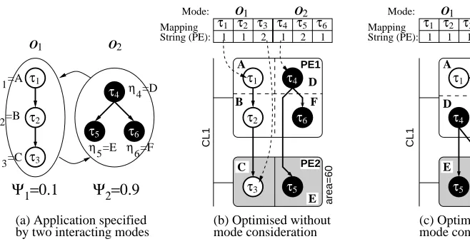
Con-sider the application shown in Figure 4(a), which consists of two operational modes, O1 and

O2, each specified by a task graph with three tasks. The system spends 10% of its operational

time in mode O1 and the remaining 90% in mode O2, i.e., the execution probabilities are given

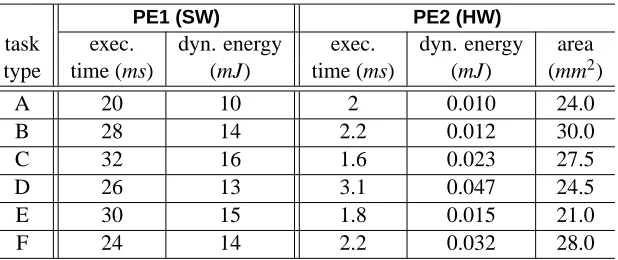
by Ψ1 =0.1 and Ψ2 =0.9. The specification needs to be mapped onto a target architecture

built of one general-purpose processor (PE1) and one ASIC (PE2), linked by a bus (CL1).

De-pending on the task mapping to either of the components, the execution properties of each task

are shown in Table 1. In general, hardware implementations of tasks achieve a higher

perfor-mance and are more energy efficient [8]. It can be observed that all tasks are of different type,

therefore, if a task is mapped to HW, a suitable core needs to be allocated explicitly for that

task. Hence, in this particular example, no hardware sharing is considered. Each allocated

core uses area on the hardware component that offers 60mm2, i.e., at most 2 cores can be

PE1 (SW) PE2 (HW)

task exec. dyn. energy exec. dyn. energy area

type time (ms) (mJ) time (ms) (mJ) (mm2)

A 20 10 2 0.010 24.0

B 28 14 2.2 0.012 30.0

C 32 16 1.6 0.023 27.5

D 26 13 3.1 0.047 24.5

E 30 15 1.8 0.015 21.0

F 24 14 2.2 0.032 28.0

Table 1: Task execution and implementation properties

that although the two modes execute mutually exclusive, the task types implemented in

hard-ware (HW cores) cannot be changed during run-time, since their implementation is static

(non-reconfigurable ASIC); as opposed to software-programmable components. Consider the mapping

shown in Figure 4(b) in which the highest energy consuming tasks (τ3andτ5, when implemented

in software) are executed using a more energy-efficient hardware implementation. According to

the task energy dissipations given in Table 1, the energy dissipation during modes O1 and O2

are E1=10mJ+14mJ+0.023mJ=24.023mJ and E2=13mJ+0.015mJ+14mJ=27.015mJ.

Neglecting the mode execution probabilities by assuming that both modes are active for even

amounts of time (50% mode 01 and 50% mode O2) energy consumption can be calculated as

Ee =0.5·24.023mJ+0.5·27.015mJ=25.519mJ. Nevertheless, taking the real behavior into

account, mode O1 is active for 10% of the operational time, i.e., its energy dissipation can then

be calculated as Er1=0.1·24.023mJ=2.4023mJ. Similarly, mode O2 is active 90% of the

op-erational time, hence, its energy is given by Er2=0.9·27.015mJ=24.3135mJ. Thus, the real

energy dissipation results in Er=Er1+Er2=26.7158mJ. Now consider an alternative mapping,

shown in Figure 4(c), for the same task graphs. In this configuration tasksτ5andτ6, i.e., the most

energy dissipating tasks of the highly active mode O2, use energy-efficient hardware

implementa-tions on PE2, while taskτ3of the less active model O1is shifted into the software-programmable

processor (PE1). According to this solution, the energy consumptions of modes O1 and O2 are

given by E1=10mJ+14mJ+16mJ=40mJ and E2=13mJ+0.015mJ+0.032mJ=13.047mJ.

Considering the even execution of each mode (neglecting the execution probabilities), the energy

consumption can be calculated as 0.5·40mJ+0.5·13.047mJ=26.524mJ. Note that this value is

higher than the corresponding energy of the first mapping (Ee=25.519mJ). Thus, a co-synthesis

approach that neglects the mode execution probabilities would optimize the system towards the

first mapping. However, in real-life the modes are active for different amount of time and hence

the real energy dissipation is given by Er=0.1·40mJ+0.9·13.047mJ=15.7423mJ. This is

41% lower compared to the first mapping (Er=26.7158mJ) shown in Figure 4(b), which is not

τ1

τ2

τ3

τ1 τ2 τ3 τ4 τ5 τ6

O2

O1

η=D 5 η6=E

η=A 1 η=B 2 η=C 3

O₁ O₂

τ3

τ2

τ1

η=A 4

τ1 τ2 τ3 τ4 τ5 τ6

O2 O1 τ2 τ3 A D E B

τ5 τ6

τ4

C

τ4

τ5 τ6

(a) Application with resource sharing possibility

(b) Resource sharing, but no shut−down possible

A D E

B

τ1

A

τ5 τ6

τ4

C (c) No resource sharing, but component shut−down

Mapping Mapping

String (PE): String (PE):

PE1

PE2 PE2

PE1

2 1 2 2 1 1 2 1 2 1 1 1

CL1 CL1

Mode: Mode:

Figure 5: Multiple task type implementations

to switch off PE2 and CL1 during mode O1, since all tasks of this mode are assigned to PE1. This

results in a significant reduction of the static power, additionally increasing the energy savings.

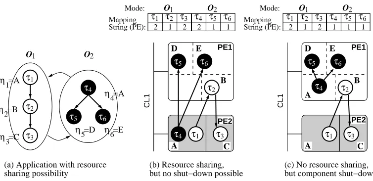
Example: Multiple Task Type Implementations

An important characteristic of multi-mode systems is that tasks of the same type might be found

in different modes, i.e., resources can be shared among the different modes in a time-multiplexed

fashion. To increase the possibility of component shutdown, it might be necessary to implement

the same task type multiple times, however, on different components. The following example,

shown in Figure 5, clarifies this aspect. Here tasks τ1 and τ4 are of type A (see Figure 5(a)),

allowing resource sharing between these tasks. The sharing is possible without contention due to

the mutual exclusive execution of these tasks (only one mode is active at a given time). In the first

mapping, given in Figure 5(b), both tasks utilize the same HW core. However, implementing task

τ4in software (additional task type A on PE1), as shown in Figure 5(c), allows to shut down PE2

and CL1 during the execution of mode O2. Hence, multiple implementations of task types can

help to reduce power dissipation.

These two examples have demonstrated that it is essential to guide the synthesis process by:

(a) an energy model that takes into account the mode execution probability as well as (b) allowing

multiple task implementations.

5

Problem Formulation

The goal of our co-synthesis approach is an energy-efficient implementation of application ϒ,

which modeled as OMSM, such that timing and area constraints are satisfied. This involves the

under the consideration of static and dynamic power as well as mode execution probabilities.

Al-though static power consumption is often neglected in system-level design approaches, since until

recently dynamic power has been the dominating power dissipation, emerging sub-micron

tech-nologies with reduced threshold voltage levels show increased leakage currents that are becoming

comparable to the dynamic currents [9]. In multi-mode systems this static power consumption can

have a significant impact on the overall energy efficiency. The reasons for this are the different

per-formance requirements of the various operational modes. For instance, the minimal perper-formance

requirements of the hardware architecture are imposed by the most computational intensive mode,

i.e., the minimal allocated architecture has to provide enough computational power to execute this

performance critical mode. However, the allocated architecture might be far more powerful than

actually needed for the execution of modes with low performance requirements. Furthermore,

low performance modes, such as the standby-mode of mobile phones (i.e., Radio Link Control),

often account for the greatest portion of the system time. During such circumstances, the static

energy dissipation of unnecessarily switched-on PEs and CLs can outweigh the dynamic energy

consumption caused by tasks of a "lightweight" mode. Thus, switching-off the unneeded

compo-nents becomes an important aspect particularly in multi-mode embedded systems. In accordance,

an accurate estimation of the average power consumption of an implementation alternative should

consider both static and dynamic power, and further the mode execution probabilities. The average

power consumption ¯p can be expressed using the following equation:

¯

p=

∑

O∈Ω

(P_Ostat+P_Odyn)·Ψ_O (1)

where P_Ostat, P_Odyn, andΨOrefer to the static power dissipation, the dynamic power dissipation, and

the execution probability of mode O, respectively. The static and dynamic power consumptions

are given as:

P_Ostat=

∑

ξ∈_KO

Pstat(ξ) (2)

and

P_Odyn=

∑

ε∈AO

Edyn(ε)

!

· 1

hpO

(3)

where Pstat(ξ)refers to the static power consumption of a componentξ, which is found in the set

of all active components

_K

P

L

also includes the additional power required for the DC/DC converter of voltage-scalable

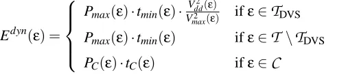
respect to the type of activities, the dynamic energy consumption Edyn(ε)can be calculated as:

Edyn(ε) =



  

  

Pmax(ε)·tmin(ε)·

V2

dd(ε)

V2

max(ε) ifε∈

T

Pmax(ε)·tmin(ε) ifε∈

T

T

PC(ε)·tC(ε) ifε∈

C

(4)

where Pmaxis the dynamic power consumption and tminthe execution time of tasks when executed

at nominal supply voltage Vmax. Tasksτ∈

T

voltage Vdd, resulting in a reduced energy consumption. Further, communications consume power

PCover a time tC. If the DVS-enabled processors are restricted to a limited set of discrete voltages,

the continuous selected supply voltage Vdd is split into its two neighboring discrete voltages Vlow

and Vhigh. The corresponding execution times in each voltage are calculated as given in [28]. The

mode execution probabilities used in Equation (1) are either based on approximations or statistical

information collected from several real users. In the case that statistical information is available

from a set of different users U , the average execution probabilities ΨO of a single operational

mode O∈Ωcan be calculated.

The co-synthesis goal is to find a task mapping M_τO, a communication mapping M_γO, a starting

time schedule S_εO, as well as a voltage schedule V_τOfor each operational mode O, such that the total

average power ¯p, given in Equation (1), is minimized and the deadlines are satisfied. Furthermore,

a feasible implementation candidate needs to fulfill the following requirements:

(a) The mapping of tasks MO_τ does not violate area constraints in terms of memory and hardware

area, i.e.,(∑_η∈Γ_πaη)≤amaxπ , ∀π∈

P

PEπ, and a_η and amax_π refer to the area used by task type ηand the available area on PE

π, respectively. Please note that for DVS-enabled HW, amax_π represents the available area including the area overhead required for the DC/DC converter.

(b) The timing schedule SO_ε and the voltage schedule V_τO, based on task and communication

mapping, do not exceed any task deadlinesθτor task graph repetition periodsφO, therefore,

tS(τ) +texe(τ)≤min(θτ,φ), ∀τ∈

T

execution time (potentially based on voltage scaling).

(c) The system reconfiguration time tT between mode changes does not exceed the imposed

maximal mode transition times t_Tmax. Hence, tT ≤tTmax, ∀T ∈Θneeds to be respected for

all mode transitions.

6

Co-Synthesis of Energy-Efficient Multi-Mode Systems

Power, Performance, Cost Evaluation

01010100101 01010001001 00100101000 01001000101 01010001001 ProbabilitiesExecution

Task & Comm. execution estimation/ profiling Allocation

Architecture

SYSTEM−LEVEL CO−SYNTHESIS

Communication Mapping

Schedulingand

Inner Loop

Outer Loop

User Driven

Dynamic Voltage Scaling and Core Allocationand Task Mapping

(OMSM) Specification

Component Shutdown

New Product Integration Hardware

Components Application_Software

Library Technology

Step 1

Step 2

Step 3

Step 4

Step 5

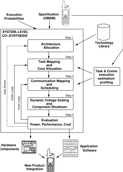
Figure 6: Multi-Mode Embedded Systems Design Flow

design flow is primarily based on two nested optimization loops. The outer loop optimizes task

mapping and core allocation, while the inner loop is responsible for the combined optimization of

communication mapping and scheduling. Although we concentrate in this paper on task mapping

and core allocation, we will outline briefly this overall design flow. As we can observe from

Figure 6, an initial system specification has to be translated into the final hardware and software

implementations. In our approach the specification includes information regarding the execution

probabilities. Along the design flow we can identify five major synthesis steps:

(1) An adequate target architecture needs to be allocated, i.e., it is necessary to determine the

quantity and the types of the different interconnected components (processing elements and

communication links). Available components are specified in the technology library.

(2) The tasks of the system specification and the require communications have to be uniquely

mapped among the allocated components. Based on the component to which a tasks has

been mapped its execution properties are determined, based on previously established

ex-ecution estimations and profiling. Furthermore, hardware cores are allocated based on the

available hardware area and the application parallelism.

(3) According to the task mapping, the communications are mapped onto the allocated

deadline, while, at the same time, achieve a good slack distribution in order to reduce

en-ergy via DVS.

(4) Dynamic voltage scaling and components shutdown possibilities are exploited to reduced

the system energy consumption.

(5) The system implementation candidates, specified by the synthesis steps 1–4, are evaluated

in terms of power consumption, performance (deadline satisfaction), cost (architecture and

hardware area). This step is used to provide feedback to the previous synthesis steps in order

to refine the design.

For more information we refer the interested reader to [30, 28, 29]. A major goal of this

de-sign flow, is to support the system dede-signer with a methodology that aids to find suitable target

architectures for a given system specification.

In this paper we concentrate on the task mapping and core allocation step, since the scheduling

and communication mapping can be carried with standard single mode techniques (e.g., [18, 29]).

This is due to the fact that the modes are executing mutually exclusive. Thus, here we present

new techniques and algorithms for task mapping, hardware core allocation, and dynamic voltage

scaling that suit the particular problems of multi-mode embedded systems. However, since these

approaches are targeted towards the exploitation of mode execution probabilities, we first discuss

how such probabilities can be obtained in practice.

6.1 Estimation of Mode Execution Probabilities

As we have demonstrated in the motivational example of Section 4, the consideration of mode

execution probabilities during design time can help to significantly reduce the energy consumption

of the embedded system. Certainly, to achieve a good design it is necessary that the execution

probabilities (estimations) used during design time reflect the real usage probabilities (in-field)

accurately. In the following, we outline how to obtain adequate execution probabilities using two

different design scenarios:

(a) The new design is an upgrade of an existing product which is connected to a service provider

(e.g. a new version of a mobile phone). For such product types it is possible to use

informa-tion regarding the activainforma-tion profile that has been collected on the provider side during the

operation of the previous product generation. For instance, the cellular network base

sta-tions can record the activation profile of the mobile terminals (e.g. phones) regarding radio

link control and calling mode, directly in-field. This information could then be evaluated

(b) The product is a completely new design. In this situation, it is common practice to evaluate

the market acceptance before the final product is introduced using a limited number of

pro-totypes that are distributed among a set of evaluation users. During this evaluation phase, the

prototypes can gather information regarding the activation profile. This information could

then be used during the final design of the product to optimize the energy consumption. Of

course, it is also possible to use application-specific insight of the designer to estimate the

execution probabilities. As we will show in the experiments given in Section 7.1, even if the

estimated execution probabilities do not reflect the user activation with absolute accuracy,

but are sufficiently close to the real values, energy savings can be still achieved.

6.2 Multi-Mode Co-Synthesis Algorithm

The task mapping approach, which simultaneously determines Mτ for all modes of application

ϒ, is driven by a genetic algorithm (GA). GAs optimize a population of individuals over several generations by imitating and applying the principles of natural selection. That is, the GA

iter-atively evolves new populations by mating (crossover) the fittest individuals (highest quality) of

the current population pool until a certain convergence criterion is met. In addition to mating,

mutation, i.e., the random change of genes in the genome (string), provides the opportunity to

push the optimization into unexplored search space regions. GA-driven task mapping approaches

have already been shown to provide a powerful tool in derive mappings for single modes systems

[16, 28]. Here we enhance such approaches towards multi-mode aspects. These enhancements

include the consideration of resource sharing, component shutdown, and mode transition issues.

As opposed to the single mode task mapping strings, such strings for multi-mode specifications

combine the mapping strings of each operational mode into one larger task mapping string, as

shown in Figure 7. Within this string each number represents the PE to which the corresponding

task is assigned. This encoding enables the usage of a genetic algorithm to optimize the placement

of tasks across the processing elements that form the distributed architecture. Please note that this

representation supports the implementation of multiple task types. For instance, if two tasks of

the same type are mapped onto different PEs, these tasks are implemented on both PEs. Thereby,

the possibility of multiple task implementations is mainly inherited into the genetic mapping

algo-rithm which is guided by a cost function that accounts for the multiple task implementations, i.e.,

the GA trades off between the savings in static power consumption against the increase dynamic

power.

The goal of the co-synthesis is to find a mapping of tasks that minimizes the total power

consumption and obeys the performance constraints. Figure 8 outlines the pseudo-code of our

co-synthesis algorithm. Starting from an initial random population of multi-mode task mapping

PE0 A B C D E F τ4 τ6 τ5 PE1 CL0 τ1 τ2 τ3 PE0 A B C D E F PE1 CL0

η₄=D

τ1 τ2 τ3 τ4 τ5 τ6 η₁=A

η₂=B

η₃=C τ3

Multi−Mode Task Mapping String η₅=E

τ4

6

τ5 τ

PE Mode2 Mode1 0 1 0 0 1 0

η₆=F τ2

τ1

Figure 7: Task mapping string for multi-mode systems

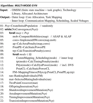
Algorithm: MULTI-MODE-SYN

Input: - OMSM (finite state machine + task graphs), Technology

Library, Allocated Architecture

Output:- Outer loop: Core Allocation, Task Mapping

- Inner loop: Communication Mapping, Scheduling, Scaled Voltages

01: Pop=CreateInitialPopulation // randomly

02:while(NoConvergence(Pop))

03: forallmap∈Pop

04: mob=ComputeMobilities(map) // ASAP & ALAP

05: cores=ImplementHWcores(map,mob)

06: ap=CalcAreaPenalty(map,cores)

07: PstatPE=CalcStaticPowerPE

08: trp=CalcTransitionPenalty(cores)

09: forallmode∈Ω

10: CommMapping_Scheduling(mode) // inner loop

11: tp(mode)=CalcTimingPenalty(mode)

12: Pdyn(mode)=CalcDynPower(mode) // incl. DVS

13: PstatCL=CalcStaticPowerCL 14: FM=MappingFitness(Pdyn,tp,PstatCL,PstatPE,ap,trp) 15: ran=RankingIndividuals(FM) 16: mat=SelectedMatingIndividuals(ran) 17: TwoPointCrossover(mat) 18: OffspringInseration(Pop) 19: ShutdownImprovementMutation(Pop) 20: AreaImprovementMutation(Pop) 21: TimingImprovementMutation(Pop) 22: TransistionImprovementMutation(Pop)

criterion is based on the diversity in the current population and the number of elapsed iterations

without producing any improved individual. To judge the quality of mapping candidates, i.e., the

fitness which guides the genetic algorithm, it is necessary to estimate important design objectives,

including static and dynamic power dissipation, area usage, and timing behavior (lines 03–13).

The following explains each of the required estimations. The hardware area depends on the

allo-cated cores on each hardware component (ASIC or FPGA). Of course, for each task type mapped

to hardware at least one core of this type needs to be allocated. However, if too many cores are

placed onto a single ASIC or FPGA, the available area is exceeded and an area penalty is

intro-duced (line 6). On the other hand, if multiple tasks of the same type are mapped to the same

hardware component and the hardware area is not violated, it is possible to implement cores

mul-tiple times (if helpful for the energy reduction). In the proposed approach, additional cores (line 5)

are allocated for parallel tasks with low mobility (line 4), therefore, the chance to exploit

applica-tion parallelism is increased. The mobility of a tasks is the difference between its earliest possible

start time and its latest possible start time [33]. Clearly, from an energy point of view this is also

preferable, especially in the presence of DVS, where a decreased execution time results in more

slack that can be exploited. Section 6.3 describes the core allocation in more detail. At this point

it is possible to compute the static power consumption of the implementation (line 7), taking into

account component shutdown between different modes. Components can be shut down during

the execution of a certain mode whenever no tasks belonging to that mode are mapped onto these

components, i.e., the component is vacant (for instance, PE0 during execution of mode O2in

Fig-ure 5). Another important aspect is the reconfigurability of FPGAs which allows to exchange the

implemented cores to suit the active mode. However, this reconfiguration during a mode change

takes time, hence, a transition penalty is introduced if the maximal transition times are exceeded

(line 8). Having determined the cores to be implemented (line 5), it is now also possible to

sched-ule each mode of the application and to derive a feasible communication mapping (line 10). Since

the modes are mutually exclusive, it is possible to employ a communication mapping and

schedul-ing optimization for a sschedul-ingle mode system. In our approach we utilize the technique described

in [28] for this step. If timing constraints are violated by the found schedule, a timing penalty is

introduced (line 11). Furthermore, based on the communication mapping and scheduling, the

dy-namic power consumption of the application can be computed, taking into account DVS (line 12)

if voltage-scalable components are present. Similarly to the shutdown of PEs, it is also possible to

switch off a CL when no communications are mapped to that link (line 13), therefore, further

re-ducing the static power consumption of the system. Based upon all estimated power consumptions

and penalties, a fitness is calculated (line 14) as,

FM=p¯·t p·(1+wA·

∑

π∈_Pv

(aU_π−amax_π )/(amax_π ·0.01))·(wR·

∏

T∈Θv

where the average power dissipation ¯p is given by Equation (1) and t p introduces a timing penalty

if the schedule exceeds task deadlines or the repetition period. Further, an area penalty is applied

for all PEs with area violation

P

transition time penalty is applied for all transitionsΘv that exceed their maximal transition time

limit, i.e., transition time tT exceeds the maximal allowed transition time tTmax. Both area and

transition penalty are weighted (wA and wR), which allows to adjust the aggressiveness of the

penalty. Having assigned a fitness to all individuals of the population, they are ranked using linear

scaling (line 15). A tournament selection scheme is used to pick individuals (line 16) for mating

(line 17). The produced offsprings are inserted into the population (line 18).

In order to improve the performance of the genetic algorithm, we apply four genetic mutation

strategies that add problem specific knowledge into the optimization process (lines 19–22). This

is achieved by introducing a small number of mutated individuals into the current population

whenever the optimization process occurs to be trapped. These newly injected solution candidates

provide the potential to turn into high quality solution by mating with other solution. The mutation

strategies are introduced next.

Shutdown Improvement: To increase the chances of component shutdown, which leads to a

reduction of static power consumption, the genetic task mapping algorithm employs a

sim-ple yet effective strategy during the optimization. Out of the current population randomly

picked individuals (probability 2% was found to lead to good results) are modified as

fol-lows. A single mode Ox and a non-essential PE πa are selected. Non-essential PEs are

considered to be PEs that implement task types that have alternative implementations on

other PEs, hence, they are not fundamental for a feasible solution. Our goal is to switch

off PE πa during the execution of mode Ox. Therefore, all tasks of mode Ox which are

mapped toπaare randomly re-mapped to the remaining PEs (

P

shut down during mode Ox. Of course, only feasible mappings are allowed, i.e., tasks are

always mapped randomly to the PEs that are capable of executing this kind of task type.

Area Improvement: To avoid convergence towards area infeasible solutions, a second strategy

is employed. If only infeasible area mappings have been produced for a certain number of

generations, the search is pushed away from this region by randomly re-mapping hardware

tasks onto software-programmable PEs.

Timing Improvement: In contrast to the area improvement strategy, if a certain amount of

tim-ing infeasible solutions have been produced, software tasks are randomly mapped to faster

hardware implementations. Thereby, the chance to find timing feasible implementations is

Transition Improvement: Cores implemented in FPGAs can be dynamically reconfigured.

How-ever, this involves a time overhead. If this overhead exceeds the imposed transition time

limits, the mapping is infeasible. Hence, after generating for a certain number of

genera-tions solely solugenera-tions that violate the transition times, tasks are randomly re-mapped away

from the FPGAs that cause the violations.

Although some of the produced genomes (strings) might be infeasible in terms of area and

timing behavior, all these strategies have been found to improve the search process significantly by

introducing individuals that evolve into high quality solutions. For instance, running the synthesis

process (on examples of moderate size) without the shutdown improvement strategy often results

in implementations which do not exploit this energy reduction possibility.

6.3 Hardware Core Allocation

For tasks mapped to ASICs and FPGAs it is necessary to allocate hardware cores that are capable

of executing the task types. This is a trivial job as long as only tasks of different types are mapped

to the same hardware component, i.e., when a single core for each task needs to be allocated.

Nev-ertheless, if tasks of the same typeηare assigned to the same PE more than once, it is necessary to

make a decision upon how many core of typeηneed to be implemented. This is important because

hardware cores are able to execute tasks in parallel, i.e., the right quantitative choice of cores can

efficiently help to exploit application parallelism, hence, improve the timing behavior as well as

energy dissipation. In the proposed co-synthesis, the following approach is employed during the

schedule optimization. Initially, each task type assigned to hardware is implemented only once,

even if multiple tasks of this type are mapped onto the same PE. This ensures that all hardware

tasks have at least one executable core implementation. If the hardware area constraints are not

violated through the initial allocation, additional cores are implemented as follows. The tasks are

analysed to identify possibly parallel executing task, taking into account task dependencies. These

tasks are then ordered according to their mobility. Clearly, tasks with low mobility are more likely

to improve the timing behavior and therefore should be the preferred choice when implementing

additional hardware cores. Accordingly, cores for task with low mobility are implemented as long

as the area constraints of the hardware components are not violated. Note that this strategy

poten-tially improves the dynamic energy dissipation, since it is probable to result in more slack time,

which, in turn, can be exploited through DVS.

6.4 Dynamic Voltage Scaling for Multiple Parallel Executing Tasks

Dynamic voltage scaling is a powerful technique to reduce energy consumption by exploiting

voltage of PEs. The applicability of DVS to embedded distributed systems was demonstrated

in [18, 22, 27]. However, these works concentrate on dynamically changing the performance of

software PEs only, while parallel execution of tasks on hardware resources has been neglected.

Nevertheless, in the context of energy-efficient multi-mode systems, where performance

require-ments of each operational mode can vary significantly, DVS needs to be considered carefully.

Consider, for instance, an inverse discrete cosine transformation (IDCT) algorithm implemented

in fast hardware which is used during two modes: MP3 decoding and JPEG image decoding.

Clearly, the JPEG decoder should restore images as quickly as possible, i.e., the IDCT hardware

is required to execute at maximal supply voltage (equivalent to peak performance). On the other

hand, the MP3 decoder works at a fixed repetition rate of 25ms for which the hardware

imple-mentation operates faster than necessary, i.e, the IDCT performance can be reduced such that this

repetition rate is adequately met. By using DVS it is possible to adapt the execution speed to suit

both needs and to reduce the energy consumption to a minimum. Here we consider that

hard-ware components might employ DVS. However, due to the area and power overhead involved in

additional DVS circuitry (DC/DC-converter [23, 15]) it is assumed that all cores allocated to the

same hardware component are fed by a single voltage supply, i.e., dynamically scaling the supply

voltage simultaneously affects the performance of all cores on that hardware component.

The new technique presented here enables an efficient usage of existing DVS approaches

[18, 22, 27] to handle the case of dynamic voltage scaling on hardware components that

exe-cute tasks in parallel. To cope with this problem, the potentially parallel executing tasks on a

single voltage-scalable hardware resource are transformed into an equivalent set of sequentially

executing tasks, taking into account the dynamic power dissipation on each core. Note that this is

done to calculate the scaled supply voltages only, i.e., this virtual transformation does not affect

the real implementation. In this section we highlight solely our transformational-based approach,

while we refer the interested reader to [18, 22, 27], where different voltage scaling techniques are

described in detail.

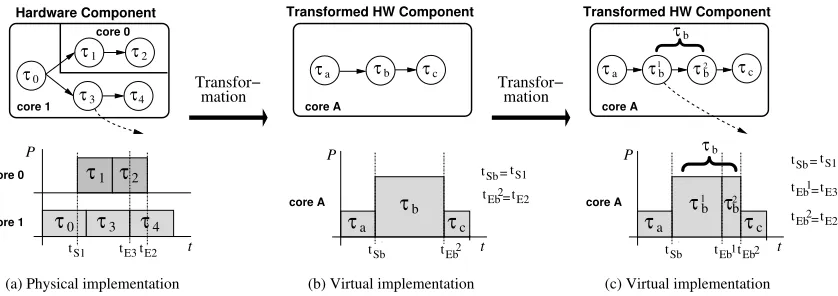
The following example illustratively outlines the proposed transformation approach. Figure 9

shows the transformation of five hardware tasks, executing on two cores (both cores are

imple-mented within the same hardware component), to four sequential tasks on a single core. The given

schedules do not only reveal the activation times of the individual tasks, but further indicate their

power dissipation over time (given by the height of the tasks). Such a power annotated schedule

is referred to as power-profile. The main advantage of the shown transformation lies within the

fact that it results in sequentially executing tasks on a single components, which is equivalent to

the behavior of software tasks. Hence, a voltage scaling technique for software processors can be

applied after the transformation, in order to exploit system idle times. Such a technique has been

τ1 τ2

τ0

τ3 τ4

τ1 τ2

τ0 τ3 τ4 tE2

tS1 tE3

mation Transfor−

mation

Transfor− τa τb τc

τa τc

τb

τb

t_Sb t_Ebt_Eb τb τb τb t_Sb t_Eb tS1 t_E3 t_E2 = = = t_Eb 1 2 core A

Transformed HW Component

P t core A 2 2 1 1 2 1

}

}

(c) Virtual implementation

τa τc t_Sb t_Eb

τb τc

τa

τb

t_Sb=t_S1 core 0 Hardware Component core 1 P t core 0 core 1

(a) Physical implementation

core A

Transformed HW Component

P

t

core A

(b) Virtual implementation

=

tEb2 tE2

2

Figure 9: DVS Transformation for HW cores considering inter-PE communication

(a) A single power profile is derived by adding the power profiles of both hardware cores and

by splitting this power profile into individual tasks whenever the power values change. In

Figure 9(b) these points are tSb(the start time of taskτ1) and tEb2 (the end time of taskτ₂).

The power dissipation of tasksτaandτcare equivalent to the power of core 1, while taskτb

dissipates a power which is the sum of the power consumptions on core 0 and core 1.

(b) Further, for each outside data dependency (indicated as dashed arrow in Figure 9), the virtual

power profile is split and additional tasks are introduced. For the given example, task τ3

communicates to an outside task. Since the execution of this task lies within the virtual task

τb, taskτb is split intoτ1_b andτ2_b. In this way the outside communication can be correctly included. Tasks with deadlines are handled in a similar fashion, in order to avoid that tasks

are extended beyond their timing constraints.

7

Experimental Results

Based on the techniques and algorithms presented in this work, a multi-mode synthesis approach

has been implemented on a Pentium III/1.2GHz Linux PC. In order to evaluate its capability to

produce high quality solutions in terms of energy consumption, timing behavior, and hardware area

requirements, a set of experiments has been carried out on 15 automatically generated multi-mode

examples (mul1–mul151) and one real-life benchmark example (smart-phone)2. All reported results were obtained by running the optimization processes 40 times and averaging the outcomes.

The average power dissipations as well as the energy consumptions have been calculated according

to Equation (1) to (4).

1_{These examples were generate with the publicly available tool TGFF [12].}

2_{The used benchmarks, including the realistic smart phone example, can be found at:}

7.1 Automatically Generated Examples

Each of the 15 generated examples (mul1–mul15) is specified by 3 to 5 operational modes, each consisting of 8 to 32 tasks (required execution cycles vary between 500–350000). The used target

architectures contain 2 to 4 heterogeneous PEs (clock frequencies are given in the range from

25 to 50MHz), some of which are DVS enabled. These PEs are interconnected through 1 to 3

communication links. The active power consumption of programmable processors was randomly

chosen between 5mW and 500mW, depending on the executed task. The power dissipation of

hardware components are selected to be 1 to 2 orders of magnitude lower. Further, the static

power dissipation was set to be 5 to 15% of the maximal active power. The execution probabilities

of individual modes were randomly chosen and vary between 1% and 85%. Timing constraints

have been assigned in the form of individual task deadlines as well as repetition periods to the

modes (hyper-periods). The timing constraints were varied between 15ms and 500ms, such that

schedulable implementations with up to 50% deadline slack could be found.

To illustrate the importance of taking mode execution probabilities into account during the

synthesis process, an execution probability neglecting approach is compared with the proposed

synthesis technique, which considers the mode probabilities. The first two sets of experiments

demonstrate the energy savings achievable through the consideration of mode execution

probabil-ities, either with or without the exploration of DVS. The third set examines the influence of the

actual activation profile on the energy savings.

Comparisons excluding Dynamic Voltage Scaling

To highlight the influence of mode execution probabilities on the achievable energy saving,

con-sider Table 2 which shows the multi-mode co-synthesis results for the 15 automatically generated

benchmarks. The first three columns give the benchmark names, the hyper-period (repetition

pe-riod) of each mode, and the mode execution probabilities. The fourth and the fifth column present

the dissipated average power and optimization time for the execution probability neglecting

syn-thesis approach. Note that the execution probabilities are neglected during the synsyn-thesis only,

while the computed power dissipations at the end of the synthesis incorporate the execution

prob-abilities, in order to ensure a meaningful comparison. The sixth and the seventh column show

the same for the proposed approach, which considers the execution probabilities throughout the

synthesis process. Take, for instance, examplemul6. When ignoring the execution probabilities

during the optimization, an average power dissipation of 1.677mW is achieved. However,

op-timizing the same benchmark example under the consideration that modes execute with uneven

probabilities (e.g., 15:10:10:65 — i.e., mode 1 is active for 15%, mode 2 is active of 10%, and

w/o probabilities with probabilities

Example Hyper- Mode Average CPU Average CPU Reduction

(No. of period Execution power time power time

modes) (ms) Probabilities (mW ) (s) (mW ) (s) (%)

mul1 (4) 70,60,90,20 5:10:75:10 8.131 20.7 7.529 24.7 7.29

mul2 (4) 50,70,40,80 10:5:80:5 3.404 15.5 2.771 18.2 18.61

mul3 (5) 20,24,60,40,30 7:3:80:5:5 10.923 23.4 10.430 23.0 4.17

mul4 (5) 60,30,70,40,50 1:4:5:40:50 7.975 21.0 6.726 25.2 15.50

mul5 (4) 20,60,60,40 7:13:35:45 5.186 18.4 4.668 22.1 10.01

mul6 (4) 65,40,40,100 15:10:10:65 1.677 20.6 1.301 19.9 22.46

mul7 (4) 200,160,190,100 5:5:5:85 3.306 11.6 1.250 21.4 62.18

mul8 (4) 400,70,40,80 75:5:15:5 1.565 32.1 1.329 28.0 15.06

mul9 (4) 40,40,100,40 7:3:80:10 3.081 6.0 1.901 5.8 38.28

mul10 (5) 500,70,500,80,70 45:5:40:5:5 1.105 28.3 0.941 32.1 14.83

mul11 (3) 100,120,200 80:10:10 2.199 9.3 1.304 16.6 40.70

mul12 (4) 80,80,90,150 15:10:50:25 7.006 25.4 5.975 34.2 14.69

mul13 (3) 80,60,100 5:15:80 4.090 15.8 2.816 15.8 31.04

mul14 (5) 60,30,60,100,190 5:5:10:10:70 8.195 28.6 6.466 33.0 21.13

mul15 (5) 220,150,60,250,200 5:10:75:7:3 2.188 41.5 1.222 55.4 44.16

Table 2: Considering mode execution probabilities (excluding DVS)

1.301mW . This is a significant reduction of 22.46%. Furthermore, it can be observed that the

proposed technique was able to reduce the energy consumption of all examples with up to 62.18%

(mul7). Note that these reductions are achieved without any modification of the underlying hard-ware architectures, i.e., the system costs are not increased. It is also important to note that the

achieved energy reductions are solely introduced by taking the mode execution probabilities into

account during the co-synthesis process, i.e., both compared approaches allow the same resource

sharing and rely on the same scheduling technique. When comparing the optimization times for

both approaches, it can be observed that the proposed technique shows a slightly increased CPU

time for most examples, which is mainly due to the more complex design space structure.

Comparisons including Dynamic Voltage Scaling

The next experiments were conducted to see how the proposed technique compares to DVS and

if further savings can be achieved by taking the mode probabilities and DVS simultaneously into

account. Table 3 reports on the findings. The DVS technique that was used here is based on

PV-DVS[27], which has been extended to enable the consideration of DVS not only for software

processors, but also for parallel executing cores on hardware PEs (see Section 6.4). As in the first

experiments, two approaches are compared here. The first approach disregards the mode execution

probabilities during optimization, while the second takes them into account throughout the

co-synthesis. Similar to Table 2, the second and the third column of Table 3 show the results without

consideration of execution probabilities, whilst the fourth and the fifth column present the results