A third order class D amplifier with and without ripple compensation

A third-order class-D amplifier with and without ripple compensation

Stephen M. Coxa, H. du Toit Moutonb

a

School of Mathematical Sciences, University of Nottingham, University Park, Nottingham NG7 2RD, United Kingdom

b

Department of Electrical and Electronic Engineering, Stellenbosch University, Private Bag X1, Matieland 7602, South Africa

Abstract

We analyse the nonlinear behaviour of a third-order class-D amplifier, and demonstrate the remarkable effectiveness of the recently introduced ripple compensation (RC) technique in reducing the audio distortion of the device. The amplifier converts an input audio signal to a high-frequency train of rectangular pulses, whose widths are modulated according to the input signal (pulse-width modulation) and employs negative feedback. After determining the steady-state operating point for constant input and calculating its stability, we derive a small-signal model (SSM), which yields in closed form the transfer function relating (infinitesimal) input and output disturbances. This SSM shows how the RC technique is able to linearise the small-signal response of the device. We extend this SSM through a fully nonlinear perturbation calculation of the dynamics of the amplifier, based on the disparity in time scales between the pulse train and the audio signal. We obtain the nonlinear response of the amplifier to a general audio signal, avoiding the linearisation inherent in the SSM; we thereby more precisely quantify the reduction in distortion achieved through RC. Finally, simulations corroborate our theoretical predictions and illustrate the dramatic deterioration in performance that occurs when the amplifier is operated in an unstable regime. The perturbation calculation is rather general, and may be adapted to quantify the way in which other nonlinear negative-feedback pulse-modulated devices track a time-varying input signal that slowly modulates the system parameters.

Keywords: Class-D amplifier, pulse-modulated systems, PWM, piecewise-smooth systems

1. Introduction

Class-D amplifiers are an important technological device and are widely used in mobile elec-tronic devices, principally because of their exceptional efficiency [1], which helps improve battery life. They operate by converting an audio signal to a high-frequency train of rectangular pulses whose widths are modulated in a manner that depends on the audio signal (pulse-width modula-5

tion, PWM) [2]. They thus inherently involve dynamics on two different time scales and so are particularly amenable to analysis by perturbation methods.

To mitigate the influence of noise, designs for class-D amplifiers generally include some form of negative feedback, and hence may be modelled mathematically as piecewise-smooth dynamical systems [3, 4]. However, while theoretical interest in such systems has primarily focused on the 10

existence, stability and bifurcations of various steady-state operating points (see, for example, [3, 4, 5, 6, 7]), here we are principally concerned with the regime of most practical interest, which is the nonlinear response to a relatively slowly varying audio input. Our goal is to understand the way in which the pulse-modulated system tracks a slowly varying input signal, with particular focus on the low-frequency components of the amplifier output.

15

In recent publications, we have explored the operation of relatively simple first- and second-order designs of class-D amplifier (with, respectively, one or two integrators in the feedback path) [8, 9, 10, 11, 12] and we have illustrated the ripple compensation (RC) technique in the first-order case [10], However, in all these cases, the operation of the feedback loop is simple enough that the entire mathematical model may be reduced to one or two nonlinear scalar difference equations 20

for the switching times of the output pulse-train. Here we treat a higher-order design, for which reduction to such a simple system is no longer possible, and the problem is formulated instead as a nonlinear system of difference equations with slowly varying forcing. Specifically, here we treat a more realistic mathematical model, with a third-order compensator in the feedback loop, and a second-order output filter, so that the state-space model for the amplifier is five-dimensional. 25

significant elements of the distortion [13, 14]. Calculation of the audio distortion is achieved by first considering the dynamics of the amplifier, specifically determining the relationship between the audio input and the switching times of the output pulse-train, then from these switching times determining the audio content of the output. Despite the algebraically involved nature of the problem, we are able to give explicit formulas for the principal components of the audio output of 35

the amplifier; these expressions make clear the contribution of the RC technique towards linearising the output.

In Section 2, we describe the amplifier treated in this paper and the RC technique; we also formulate the state-space model for the device. In Section 3, we calculate the steady-state (time-periodic) operating point of the device in response to a constant input, and briefly consider its 40

stability in Section 4. This stability calculation informs the choice of parameter values for later simulations (our goal is not to explore instability and bifurcation, rather to ensure that the device is operated in a stable regime of practical relevance). In Section 5, we develop a small-signal model which yields a transfer function relating small disturbances at the input to the consequential small disturbances at the output. This small-signal model allows us to deduce certain aspects 45

of the behaviour of the device in response to a full audio signal, and in particular shows the linearising effect of RC. The principal results of this paper are contained in Section 6, where we carry out a large-signal perturbation calculation of the amplifier output, where the perturbation parameter is proportional to the ratio between typical time scales for the output switching and the audio signal. We corroborate our theoretical results with corresponding simulations, which 50

are presented in Section 7. Besides simulations in the stable regime of practical interest, we illustrate the calamitous sudden increase in the audio distortion that arises when the parameters of the device are poorly chosen, so that the steady-state operating point is unstable. Finally, we close, in Section 8, by summarising our results and emphasising that our analysis — in particular the asymptotic calculation of Section 6 — may be applied to a wide range of negative-feedback 55

u

(

t

)

+

H

m

(

t

)

−

+

g

(

t

)

v

(

t

)

k

+

G

f

(

t

)

−

+

+

+

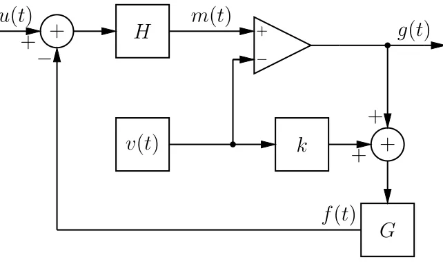
Figure 1: Third-order amplifier. The input audio signal isu(t). G represents the transfer function of the output

filter. There is ripple compensation (RC) ifk= 1; otherwise, ifk= 0, there is no RC. The amplifier output isg(t).

The compensator is denoted byH. The output of the compensator, denoted bym(t), is fed into the positive input

of the comparator, whose negative input receives the sawtooth wavev(t). The output takes the values±1 according

to the sign ofm(t)−v(t).

2. Mathematical formulation

Figure 1 shows the amplifier. The output g(t) is a rectangular wave taking the values ±1 according to

g(t) = sgn(m(t)−v(t)),

wherem(t) andv(t) are, respectively, the noninverting and inverting inputs of a comparator. The 60

rising edges of g(t) occur at regular intervals, where t= nT and the constant T is the period of the carrier wave v(t). The falling edges ofg(t) occur at times that vary according to the output

m(t) of the compensator, as illustrated in Figure 2. We denote these modulated down-switching times byAn, so that

g(t) =

  

 

+1 for nT < t < An,

−1 forAn< t <(n+ 1)T.

(1)

The sawtooth carrier wave is given by 65

(

n

₋

1)

T

A

nT

A

g

(

t

)

t

t

v

(

t

)

m

(

t

)

(

n

−

1)

T

A

nT

A

t

g

(

t

) +

v

(

t

)

(

n

+ 1)

T

Figure 2: Signalsg(t),v(t),m(t) andg(t) +v(t). The rising switching edges ofg(t) occur regularly, at timest=nT;

the falling switching edges occur at times t = An, where m(An) = v(An). (The signal m(t) is for illustrative

purposes.) The signalg(t) +v(t) is a linear ramp, with falling switching edges at timest=An.

fornT ≤t <(n+ 1)T (with v(t+T) =v(t) for all t), and hence the condition for switching is

m(An) =−1 + 2an, where an= (An−nT)/T. (2)

The low-pass filter G receives as input g(t) +kv(t), where k is either 0 or 1. The choice k = 0 indicates that RC is not applied; we note that in this case the filter input isg(t), which is piecewise constant, switches up at times t = nT and down at times t =An. Otherwise, the choice k = 1

corresponds to the application of RC; the filter input is nowg(t) +v(t), which is a piecewise linear 70

upwards ramp, which switches down at times t = An, as in Figure 2. (Note that G represents

the output filter; its repositioning into the feedback loop, as in Figure 1, may be achieved through standard block-diagram manipulations — for example, see Figure 5 of [13].)

The motivation for the RC technique is the observation that feedback of the output ripple signal leads to a nonlinearity in the PWM process: high-frequency carrier components are aliased to the 75

−

g

(

t

) +

kv

(

t

)

+

L

C

R

+

f

(

t

)

−

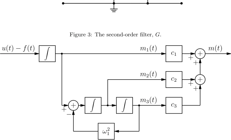
Figure 3: The second-order filter,G.

u(t)−f(t) ! m1(t)

c1 +

+

! !

m2(t)

c2

m(t)

ω₁2

m3(t)

c3

+

−

+

+ +

+ +

Figure 4: The third-order compensator,H.

Section 3 of [13], but the key to the success of RC in reducing output distortion may be illustrated with the following observations regarding the steady-stateT-periodic response of the amplifier to a 80

constant inputu(t) =u0. Whenk= 0, the steady-state duty cyclean≡avaries according to the

amplifier inputu0; for different values ofa, the shape ofg(t) is thus different, and hence the shape

of the compensator output varies accordingly. Put differently, the ripple depends on the inputu0.

By contrast, with RC the shape of g(t) +v(t) is same regardless of the value of u0, except for a

u0-dependent time shift and the addition of a u0-dependent constant to the values ofg(t) +v(t).

85

Put differently, as we shall make precise below, in Section 3.1, with RC the ripple is in essential respects independent of u0.

2.1. State-space model

We next present the ordinary differential equations that govern the operation of the device. We begin by examining the action of the low-pass filter G, shown in Figure 3. We let f(t) = 90

(f(t), f′

a vector or matrix, and the prime denotes the time derivative. Then

f′(t) =M2f(t) +

g(t) +kv(t)

LC (0,1)

T_{, (3)}

where

M2=



 

0 1

−(LC)−1 −(RC)−1





.

The filter may equivalently be specified in terms of its (Laplace) transfer function

G(s) = 1/(LCs2+Ls/R+ 1).

Next we turn to the compensator H, which comprises a chain of integrators with feed-forward 95

summation and a local resonator feedback loop, shown in Figure 4. We introduce the state vector m(t) = (m1(t), m2(t), m3(t))T. Then

m′(t) =M3m(t) + (u(t)−f(t))(1,0,0)T, (4)

where

M3 =



    

0 0 0

1 0 −ω₁2

0 1 0



     .

The output of the compensator is

m(t) =c1m1(t) +c2m2(t) +c3m3(t),

for some constantsc1,c2,c3. The (Laplace) transfer function of the compensator is

100

H(s) = c1

sT +

c2

(ω2

1+s2)T2

+ c3

(ω2

1+s2)sT3

.

We solve the systems (3) and (4) together, by introducing the state-space vector

x(t) = (m1(t), m2(t), m3(t), f(t), f′(t))T,

which is governed by

x′(t) =Nx(t) +u(t)e1+

g(t) +kv(t)

wheree1 = (1,0,0,0,0)T, . . . , e5= (0,0,0,0,1)T. The matrix N is partitioned as follows: N =              M3

−1 0 0 0 0 0 0 0 0

0 0 0

M2              .

To simplify the analysis here and in later sections, we next diagonalise N. We thus introduce the diagonal matrix Λ of the eigenvalues ofN, which are 0, iω1,−iω1,−µ+ iΩ and−µ−iΩ, where

105

µ= 1

2RC, Ω = r

1

LC −

1 4R2_C2.

We also introduce a matrix R whose columns are given, respectively, by the corresponding right eigenvectors ofN: w1, . . . , w5. Then

N =RΛR−1. (6)

The rows of R−1 _{are the left eigenvectors of N: v}

1, . . . , v5. Of particular utility in our analysis

will be the left zero eigenvector

v1 = (−(LC)−1,0,0,(RC)−1,1). (7)

Correspondingly,w1 = (−LC,0,−LC/ω21,0,0)T.

110

To simplify later notation when we integrate (5), we introduce Pn(t) andQn(t), where

P0(t) = eN te1, and Pn+1(t) =

Z t

0

Pn(τ) dτ (8)

forn= 0,1, . . .;

Q₀(t) = eN te5, and Qn+1(t) =

Z t

0

Q_n(τ) dτ

forn= 0,1, . . .. We find

Pn(t) =

tn

n!e1+φn(t)e2+φn+1(t)e3,

whereφ−₁(t) = cosω₁t and

φn+1(t) =

Z t

We may readily integrate (5) over any time interval [t0, t1], to give

115

x(t1) = eN(t1−t0)x(t0) +

Z t1

t0

eN(t1−τ)_e

1u(τ) dτ +

1

LC Z t1

t0

eN(t1−τ)_e

5(g(τ) +kv(τ)) dτ. (9)

For later purposes, our specific interest is in integrating (5) over the interval [An, An+1] between

successive falling edges of the amplifier outputg(t). To evaluate the first integral in (9), we begin by writing

Iu,n≡ Z An+1

An

eN(An+1−τ)_e

1u(τ) dτ.

Then Taylor expansion of u(τ) about τ = An and repeated use of integration by parts on the

result, together with (8), gives 120

Iu,n= ∞ X

k=0

Pk+1(An+1−An)u(k)(An), (10)

where the superscript denotes the k-th derivative. The second integral in (9) is similarly found (after just one integration by parts, to deal with v(τ)) to be

Ig,v,n ≡

Z An+1

An

eN(An+1−τ)_e

5(g(τ) +kv(τ)) dτ

= 2(1−k)Q₁(an+1T) + (−1−k+ 2kan)Q₁(An+1−An) +

2k

T Q2(An+1−An).

Assembling these results, we thus arrive at the discrete-time model

x(An+1) = eN(An+1−An)x(An) +Iu,n+

1

LCIg,v,n, (11)

together with the switching condition (2), which becomes

γTx(An+1) =−1 + 2an+1, (12)

where 125

γT = (c1, c2, c3,0,0).

The system (11), (12) forms the basis for our mathematical analysis of the amplifier. We note that this system may be reduced to a single (fifth-order, nonlinear) scalar difference equation for

an (cf. [16]). However, while we shall make use of a related reduction later, in Section 6, the bulk

3. Steady-state operation 130

We begin our analysis of the mathematical model set out above by examining its steady-state behaviour in response to a constant input. This is necessary in order for us to choose suitable parameter values for our simulations, where the steady-state response should be stable; it also sheds some light on the operation of RC.

We thus suppose that u(t) = u0 and that all signals are T-periodic. In particular all duty

135

cycles are equal, withan≡a. In such steady-state operation, (11) becomes

(I5−eN T)x(aT) =Φ(a, T), (13)

whereI5 is the 5×5 identity matrix,

Φ(a, T) =u0P1(T) +

1

LC

2(1−k)Q₁(aT) + (−1−k+ 2ka)Q₁(T) +2k

T Q2(T)

,

and the switching condition isγTx(aT) =−1 + 2a. Note that the matrix on the left-hand side of (13) is singular, and after left-multiplying byv1, given in (7), we obtain the solvability constraint

v1Φ(a, T) = 0; (14)

this then yields the duty-cycle condition 140

a= 1₂(1 +u0), (15)

which expresses the fact that the time-averaged outputhg(t)i=u0.

Once the duty-cycle condition (14) has been imposed, it remains to determine x(aT), from which the entire periodic solution may subsequently be obtained using (9). This is accomplished by replacing one row (for example, the first) of the vector equation (13) with the switching condition (12); thus we solve

145

˜

Mx(aT) = ˜Φ,

where

˜

Mij =

     

    

cj fori= 1 and j= 1,2,3,

0 fori= 1 and j= 4,5, (I5−eN T)ij fori= 2,3,4,5

and

˜ Φi =

  

 

Explicit formulas for the steady-state solution are too algebraically involved to record here. A quantity of particular significance in our later stability calculation and in our development of a model for small disturbances to the steady state is the slope of the compensator output at the 150

modulated switching instant; thus we note from (5) that this slope is

m′(aT) =γTx′(aT) =γTNx(aT) +c1u0. (16)

3.1. Relation between steady-state operating points for different inputs (with ripple compensation)

With RC, there is a particularly simple relationship between the steady-state operating points for different values of the input u0, which we elucidate in this section. The simplicity of this

relationship underpins the effectiveness of RC in reducing the amplifier’s inherent distortion. 155

We consider two different T-periodic steady-state solutions, with different values of u0, and

hence different switching times forg(t) +v(t). For each solution, the duty-cycle condition (15) is satisfied, together with the state-space equation (5) and the switching condition (12). Thus the two solutions, xa(t) and xb(t), satisfy

x′_a(t) =Nxa(t) + (2a−1)e1+

2

LC(−1 +t/T)e5 foraT ≤t < aT +T ,

γTxa(aT) =−1 + 2a

(17)

and 160

x′_b(t) =Nxb(t) + (2b−1)e1+

2

LC(−1 +t/T)e5 forbT ≤t < bT +T ,

γTxb(bT) =−1 + 2b.

(18)

To demonstrate the relationship between the two solutions, we introduce theT-periodic quantity ∆(t) =xb(t+ (b−a)T)−xa(t),

which satisfies

∆′(t) =N∆(t) + 2(b−a)

e1+

1

LCe5

foraT ≤t < aT +T ,

γT∆(aT) = 2(b−a).

(19)

The general solution to the ODE in (19) is

∆(t) = eN(t−aT)∆(aT) + 2(b−a)

Z t

aT

eN(t−τ)ǫdτ, (20) where

ǫ=e1+

1

From (20), we see that 165

N∆(t) = eN(t−aT)N∆(aT) + 2(b−a)eN(t−aT)−I5

ǫ,

which may be rearranged as

X(t) = eN(t−aT)X(aT), (21) where

X(t) =N∆(t) + 2(b−a)ǫ. (22) Since X(t) isT-periodic, it follows from (21) witht=aT +T that

eN T −I5

X(aT) =0. (23)

Hence X(aT) =X3w1 for some constant X3. The value ofX3 may be determined from (22): we

see that 170

v1X(aT) =v1N∆(aT) + 2(b−a)v1ǫ= 0,

hence (considering leftmost and rightmost sides of this equation)X3 = 0. ThusX(aT) =0, and

from (21) it follows that X(t)≡0, so that, from (22),

∆(t) = (ω2₁,0,1,0,0)T∆3(t) + (0,0,0,2(b−a),0)T,

for some ∆3(t). Substitution in (19) shows that∆(t) is in fact constant. Then from the switching

condition in (19) we see that (c1ω12+c3)∆3 = 2(b−a), hence

∆= 2(b−a)

c1ω21+c3

ω₁2,0,1, c1ω21+c3,0

T

.

In summary, we have shown that, for aT ≤t < aT +T, 175

xb(t+ (b−a)T) =xa(t) +∆.

Since the two steady-state solutions differ by the addition of a constant vector, and by time-shifting, the derivatives of each solution around the modulated switching instant agree: more specifically,

γTx′_b(bT) =γTx′_a(aT).

This fact has significant consequences, as we shall see later, in Section 5, when we show how it leads to a linearisation of the small-signal model.

4. Stability of the steady-state operating point

Our interest is in stable operation of the amplifier, so we provide just a brief discussion of stability considerations. Following Aizerman and Gantmakher [17] (see also, for example, [3, 7, 18]), we suppose that the input u(t) =u0 is fixed, and consider the growth or decay of a perturbation

to the steady state over the intervalt∈[0, T]. We write 185

x(t) = ¯x(t) + ∆x(t), a0=a+ ∆a,

where ¯x(t) is the steady-state solution with duty cyclea. Then, upon linearising in small distur-bances, we find

∆x(T) = eN(1−a)T

I5+ T κ

LCe5γ

T_eN aT

| {z }

≡M

∆x(0), (24)

where

κ= (1−1₂TγTx¯′(aT))−₁

, (25)

and the quantityγTx¯′

(aT) may be obtained from (16). The stability of the steady-state operating point is thus determined by the eigenvalues of the matrix M [3]. Note that the sole difference 190

between the RC and no-RC versions ofMlies in the value of κ. The eigenvalues µof Msatisfy

det(M −µI) = 0. (26)

We may derive an alternative equation for these eigenvalues (cf. [7, 19, 20]), which may be more useful in some cases, by use of Sylvester’s Determinant Theorem [21], which states that det(In− AB) = det(Ip−BA), where A is anyn×pmatrix andB is anyp×nmatrix, andIn and Ip are,

195

respectively,n×nandp×pidentity matrices. We suppose, as is readily verified, that none of the eigenvalues of exp(N T) are also eigenvalues of M. Then

det(M −µI) = det(eN T −µI+αβT) = det(eN T −µI) det(I + (eN T−µI)−1αβT),

where

α= T κ

LCe

N(1−a)T_e

5, βT =γTeN aT.

Hence the eigenvaluesµ ofM satisfy

and so, by Sylvester’s Determinant Theorem, they also satisfy the equation 200

1 + T κ

LCγ

T_eN aT_(eN T _−µI)−₁

eN(1−a)Te5 = 0,

or, equivalently,

1 + T κ

LCγ

T_Rdiag(eλjT_/(eλjT _−µ))R−1_e

5 = 0, (28)

where λj are the eigenvalues of N. We use either (26) or (28) to choose parameter values for

our simulations (see Section 7) so that the steady-state operating point is stable, unless otherwise stated.

5. Small-signal model 205

The stability analysis of Section 4 may be generalised to give a small-signal model that relates small disturbances at the input to the corresponding small disturbances at the output. We suppose that some small time-dependent perturbation is superposed on an otherwise steady input, so that

u(t) =u0+ ∆u(t). We introduce the notation ¯An= (n+a)T for the unperturbed switching times,

and write the perturbed switching times as An = ¯An+ ∆anT. We write x(t) = ¯x(t) + ∆x(t)

210

accordingly. We linearise in all small quantities.

In what follows, we assume that the n-th switching instant is delayed, so that ∆an>0. This

is simply to fix the time-ordering of various events; the resulting expressions for the small-signal model do not rely on this assumption, and apply equally well if that switching instant is instead advanced, so that ∆an<0.

215

We note that ¯x(t) depends on the value ofk. By contrast, for the perturbations, regardless of whether k= 0 or 1, we have the following governing equations: on ( ¯An,A¯n+ ∆anT),

∆x′(t) =N∆x(t) + ∆u(t)e1+

2

LCe5;

on ( ¯An+ ∆anT,A¯n+1),

∆x′(t) =N∆x(t) + ∆u(t)e1.

Integration of these differential equations in turn gives ∆x( ¯An+1) = eN T

∆x( ¯An) +

2∆anT

LC e5

+

Z T

0

eN τ∆u( ¯An+1−τ)e1dτ. (29)

The linearised switching condition (12) yields 220

where againκ is given by (25). We note that whenk= 0,κ depends onu0, whereas when k= 1,

κ is independent of u0.

Through repeated integration by parts, as in the derivation of (10), it may be established, using (29) and (30), that

∆x( ¯An+1) =N∆x( ¯An) + ∞ X

m=0

Pm+1(T)∆u(m)( ¯An), (31)

where 225

N = eN T

I5+

T κ

LCe5γ

T_.

(Note thatM= e−N aTNeN aT, whereMis defined in (24), hence Mand N are similar matrices and so share the same eigenvalues.)

A recurrence relation for the switching-time perturbation may now be derived by premultiplying (31) by 1₂κγT then using (30). A convenient formulation for the solution may be obtained by introducing the derivative operator D≡d/dt and using the Taylor expansion [22, 23]

230

∆x( ¯An+1) = eTD∆x( ¯An),

to give the formal solution

∆an= 1₂κγT

eTDI5− N

−1 X∞

m=0

Pm+1(T)∆u(m)( ¯An). (32)

The next step is to characterise the corresponding spectral components of the output pulse-train. To this end, we letx(t) be such thatx( ¯An) = ∆an. In view of (32), one particular choice of x(t) satisfies

x(t) = 1₂κγT eTDI5− N

−_{1 X}∞

m=0

Pm+1(T)∆u(m)(t). (33)

The final step in our derivation of the small-signal model uses x to reconstruct the amplifier 235

output. From (1), it follows that the Fourier transform of the full output g(t) is ˆ

g(ω) =

Z ∞

−∞

e−iωtg(t) dt= 2 iω

∞ X

n=−∞

e−iωnT −e−iωAn_,

where the last inequality holds for ω 6= 0. By considering the difference between the Fourier transform of the output with and without perturbation, we find that the perturbation to the output has Fourier transform (forω6= 0)

∆ˆg(ω) = 2 iω

∞ X

n=−∞

Linearisation in small perturbations then gives 240

e−iωAn _{= e}−iωA¯n_e−iω∆anT _∼e−iωA¯n_(1−iω∆a

nT).

(In the time domain, this linearisation is tantamount to replacing the narrow rectangular pulses in ∆g(t) by Dirac δ-functions.) Thus (34) becomes

∆ˆg(ω) = 2T ∞ X

n=−∞

e−iωA¯n_{x( ¯A}

n) = 2 ∞ X

n=−∞

e−2πniaxˆ(ω−2πn/T), (35) where the second equality follows from Poisson resummation [24].

There is no particular restriction on the bandwidth of the input perturbation signal for (35) to be valid. However, further mathematical progress is substantially eased if we make the physically 245

reasonable assumption that the input perturbation ∆u(t) contains only audio frequencies, so that ∆u(t) (and hence also x(t)) is band-limited, with ∆ˆu(ω) = ˆx(ω) = 0 for |ω| ≥ π/T; then, from (33) and (35),

∆ˆg(ω) =κγTeiωTI5− N

−1 X∞

m=0

Pm+1(T)(iω)m∆ˆu(ω)

for|ω|< π/T. To simplify the sum in this expression, we let

σ(T; iω) =

∞ X

m=0

Pm+1(T)(iω)m,

then note that in consequence 250

dσ(T; iω)

dT −iωσ(T; iω) =P0(T), σ(0; iω) =0.

Solving this ODE, we thus have

σ(T; iω) =σ1e1+σ2e2+σ3e3,

where

σ1 =

eiωT ₋₁

iω ,

σ2 =

iωsinω1T−iω1sinωT +ω1(cosω1T−cosωT)

ω1(ω2−ω21)

,

σ3 =

ωsinω1T −ω1sinωT

ωω1(ω2−ω12)

+ iω

2

1cosωT −ω2cosω1T+ω2−ω21

ωω2

1(ω2−ω21)

.

This, finally, yields the (input–output) transfer function, from ∆ˆu(ω) to ∆ˆg(ω), which is

κγT eiωTI5− N

−₁

for “audio frequencies” (those less thanπ/T in magnitude).

Without RC, this transfer function depends on u0, through the value ofκ (both explicitly in

255

(36) and implicitly through N) and so the small-signal model predicts an inherently nonlinear response for the amplifier. This is undesirable, since such nonlinearity leads to unwanted total harmonic distortion (THD) and intermodulation distortion (IMD) [12, 25].

With RC, the transfer function is independent of u0, so we expect it to provide an accurate

characterisation of the input–output relation even for inputs that are not small perturbations to

260

some constant input. This is a striking result, because it predicts an essentially linear behaviour for the amplifier. More specifically, for an audio input u(t), the small-signal model predicts an output with audio-frequency Fourier components given by

ˆ

ga(ω) =κγT

eiωTI5− N

−1

σ(T; iω)ˆu(ω).

In fact, as we shall demonstrate in the next section, the full audio output isnot quitelinearly related to the input: harmonics are generated, but from terms neglected in the small-signal linearisation 265

(cf. [10]). An example of such a term is ((u′

)2)′

, which involves a product of input derivatives; the contribution of such terms is, however, small [10].

We next turn to a full calculation of the output that is not constrained by the linearisation inherent in the small-signal model.

6. Fully nonlinear model 270

Our final calculation gives the nonlinear audio output in response to a general audio input. This calculation tracks the slowly changing operating point of the amplifier in response to its input, in sufficient detail to allow us to find the principal contributions to the output distortion. Of necessity, it avoids the traditionalquasi-steadyengineering approximation, that the input to the amplifier is assumed constant over any switching cycle. We follow the structure of the calculation 275

described in [8, 9, 10, 11, 12], although here the details are considerably more algebraically involved than in any of those previous cases. We emphasise that our approach may be readily adapted to other pulse-modulated feedback systems [4] with slowly varying input parameters.

We apply a perturbation method based on the small parameter

whereω is a typical audio frequency. We introduce a correspondingly scaled time 280

τ =ωt=ǫt/T.

Thus variations to the audio input occur on a time scale τ =O(1), while the switching time scale hasτ =O(ǫ). We introduce

U(τ) =u(t),

so thatu(m)(t) = (ǫ/T)mU(m)_{(τ). Our interest is in determining how solutions to the system (11),}

(12) track the slow parametric variation afforded by the input audio signal.

We first determine the way in which the switching times depend on the audio input, then 285

calculate the corresponding audio output. To this end, we introduce functions aandX _{such that}

a(ǫn) =an, X(ǫn) =x(An) =x((n+a(ǫn))T).

Writing the difference equation (11) and switching condition (12) in this notation, we find that each equation involves a(ǫn) or a(ǫ(n+ 1)). Clearly these equations are expected to hold only for integer values ofn. However, as a mathematical device to enable a solution to be obtained, we seek to impose each equation for all real values of n (since if we are able to do so then the equations 290

certainly hold when restricted to integer n). Thus we setτ =ǫn and solve for allτ the following: X_{(τ +ǫ) = e}N dτ_{X(τ) +Θ(τ), γ}T_{X(τ) =−1 + 2a(τ), (37)} where

Θ(τ) =

∞ X

m=0

ǫm

TmPm+1(dτ)U

(m)_{(τ +ǫa(τ)) +} 2(1−k)Q1(a(τ +ǫ)T)

LC

−(1 +k−2ka(τ))Q1(dτ)

LC +

2k

T LCQ2(dτ)

and where

dτ = (1 +a(τ +ǫ)−a(τ))T.

The functions aand X _{are then expanded in powers of ǫ, and coefficients of successive powers of}

ǫequated in (37). 295

Given the algebraic complexity of the perturbation problem, it is useful to reduce the problem from the six scalar equations represented in (37) to a single scalar equation, fora(τ) (cf. [16]). To do so, we introduce

Then the first of (37) becomes

V_{(τ+ǫ) = e}N TV_{(τ) + e}−a(τ+ǫ)N T_Θ(τ), so that

300

eǫDI5−eN T

V_{(τ) = e}−a(τ+ǫ)N T_{Θ(τ), (39)} where throughout this section D denotes d/dτ.

Then, using (6), (39) may be written as

ReǫDI5−eΛT

R−1V_{(τ) =Re}−a(τ+ǫ)ΛT_R−1_Θ(τ),

so that

V_{(τ) =Re}ǫD_I5−eΛT

−₁n

e−a(τ+ǫ)ΛTR−1Θ(τ)o. (40) Using (38) and (40), we see that the switching condition in (37) becomes

γTea(τ)N TReǫDI5−eΛT

−1

e−a(τ+ǫ)ΛTR−1Θ(τ)=−1 + 2a(τ), (41) which is the promised single scalar equation for a(τ).

305

Several of the terms in this equation may readily be simplified, by introducing the Bernoulli numbers Bn and the Bernoulli–Apostol functions βn [26], which satisfy the following generating

functions (for γ 6= 1):

z

ez₋₁ = ∞ X

n=0

Bn

n!z

n_, z

γez₋₁ =

∞ X

n=1

βn(γ)

n! z

n_.

Thus

D ≡eǫDI5−eΛT

−₁

= diag(ζ1, ζ(iω1), ζ(−iω1), ζ(−µ+ iΩ), ζ(−µ−iΩ)),

where 310

ζ1 =

1 ǫD ∞ X n=0 Bn

n!(ǫD)

n_{, ζ(z) = e}−zT ∞ X

n=0

βn+1(e−zT)

(n+ 1)! (ǫD)

n_,

and the equation for a(τ) simplifies from (41) to

γTRea(τ)ΛTDne−a(τ+ǫ)ΛTR−1Θ(τ)o=−1 + 2a(τ). (42) From the Fourier transform of (1), it may be deduced [8, 9, 10, 11] that the audio contribution to the output (i.e., the contribution involving frequencies less than π/T) is

ga(t) =−1 + 2 ∞ X

n=0

(−ǫ)n

(n+ 1)!

dn_an+1_(τ)

and so, in principle, the required calculation is now clear: we expanda(τ) in powers of ǫ, as

a(τ) =a0(τ) +ǫa1(τ) +O(ǫ2), (44)

then solve (42) at successive powers of ǫ to find in turn the an(τ), finally substituting these

315

expressions in (43) to determine the output. In practice, of course, the details are extremely algebraically cumbersome. The next section describes this calculation at the first two orders inǫ; these provide the principal contributions to the audio output.

6.1. Calculation of the output to O(ǫ)

From (43), we see that the output takes the form 320

ga(t) =−1 + 2a0(τ) +ǫg1+O(ǫ2), (45)

where

g1 = 2a1(τ)−2a0(τ)a′0(τ). (46)

In solving (42) fora0(τ) and a1(τ), we need the following expansions:

ea(τ)ΛT = ea0(τ)ΛT _+ǫa

1(τ)ea0(τ)ΛTΛT+O(ǫ2),

e−a(τ+ǫ)ΛT = e−a0(τ)ΛT _−ǫ(a

1(τ) +a′0(τ))e

−a0(τ)ΛT_ΛT+O(ǫ2_).

We also expand

eǫDI5−eΛT

−1

= 1

ǫDΥ−1+ Υ0+O(ǫ),

where Υ−₁ = diag(1,0,0,0,0) and

Υ0 = diag(−1/2,(1−eiω1T)−1,(1−e−iω1T)−1,(1−e(−µ+iΩ)T)−1,(1−e(−µ−iΩ)T)−1).

WritingΘ(τ) =Θ0(τ) +ǫΘ1(τ) +O(ǫ2), we find that

325

Θ0(τ) =P1(T)U(τ) +

2(1−k)Q₁(a0(τ)T)

LC −

(1 +k−2ka0(τ))Q1(T)

LC +

2k

T LCQ2(T)

and

Θ1(τ) =

1

TP2(T)U

′

(τ) +P1(T)a0(τ)U′(τ) +TP0(T)a′0(τ)U(τ)

+2 (kQ1(T) + (1−k)TQ0(a0(τ)T)) (a1(τ) +a

′

0(τ))

LC −

(1 +k−2ka0(τ))TQ0(T)a′0(τ)

The leading terms in (42) are those at O(ǫ−₁

), which give

γTRea0(τ)ΛT_D−1n_Υ

−1e−a0(τ)ΛTR−1Θ0(τ)

o

= 0. (47)

This equation may be considerably simplified by noting that Υ−₁e−a0(τ)ΛT = Υ−₁ and, further,

that

Υ−₁e−a0(τ)ΛTR−1 =R, (48)

whereR is a 5×5 matrix whose first row isv1 and whose remaining elements are all zero. Thus

330

we may satisfy (47) by imposing the condition

v1Θ0(τ) = 0. (49)

It is readily established that

v1Pn(t) =−

tn

n!LC, v1Qn(t) =−

tn

n!,

and hence, from (49),

a0(τ) = 1₂(1 +U(τ)), (50)

which is the analogue of the duty-cycle condition (15).

The next terms to consider in (42) are those at O(1). After benefiting from the considerable 335

simplification that follows from using (48) and imposing (49), we find γTRea0(τ)ΛT_Υ

0e−a0(τ)ΛTR−1Θ0(τ) + D−1RΘ1(τ)

=−1 + 2a0(τ).

Then, since exp(±a0(τ)ΛT) and Υ0 are all diagonal matrices, we see that

ea0(τ)ΛT_Υ

0e−a0(τ)ΛT = Υ0;

furthermore, ea0(τ)ΛT_{R=R. Thus, by making use of these results and (48), we have}

γTRΥ0R−1Θ0(τ) + D−1RΘ1(τ)

=−1 + 2a0(τ),

which we may solve by taking

γTRRΘ1(τ) =U′(τ)−γTRΥ0R−1Θ′0(τ), (51)

where we have used (50) to eliminate a0(τ).

Now RΘ1(τ) = (θ1,0,0,0,0)T, where

θ1 =v1Θ1(τ) =

T LC

g1−

1

2(1−k)U(τ)U

′

(τ)

,

whereg1 is defined in (46). Furthermore, elementary matrix algebra gives γTRRΘ1(τ) =θ1γTw1=−

LC

ω2

1

(c1ω21+c3)θ1.

The right-hand side of (51) may be expressed more concretely by noting that Θ′₀(τ) =P1(T)U′(τ) +

(1−k)T

LC Q0(a0(τ)T)U

′

(τ) + k

LCQ1(T)U

′

(τ).

If we now define

pn(t) =γTRΥ0R−1Pn(t), qn(t) =γTRΥ0R−1Qn(t),

theng1 is given by

345

g1 = (1−k)U(τ)U

′

(τ)

2 −

ω2₁(1−ψ(τ))U′

(τ) (c1ω21+c3)T

, (52)

where

ψ(τ) =p1(T) +

(1−k)T

LC q0(

1

2(1 +U(τ))T) +

k

LCq1(T).

This expression for g1 enables us to determine the most significant components of the audio

dis-tortion.

We note that without RC (i.e., for k = 0) the expression for g1 is nonlinear in U, and hence

the output contains harmonic distortion at O(ǫ). We also see that with RC (k= 1) g1 becomes

350

the much simpler expression

g1 =−

ω2₁(1−p1(T)−q1(T)/(LC))

(c1ω21+c3)T

U′

(τ),

which involves only terms that are linear inU (the first nonlinearterms, involving quantities such as ((U′

)2)′, which involve three derivatives, will arise first at O(ǫ3) in the output, cf. [10]).

Thus we have determined explicitly (at least, to O(ǫ)) the way in which the nonlinear be-haviour of the amplifier tracks the slowly varying audio input, and in particular the resulting 355

low-frequency components of the output. While the leading-order tracking result, from (45) and (50), that ga ∼ U, is well known and is easily understandable from the duty-cycle balance in

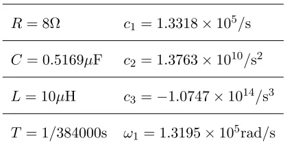
R= 8Ω c1 = 1.3318×105/s

C= 0.5169µF c2 = 1.3763×1010/s2

L= 10µH c3 =−1.0747×1014/s3

T = 1/384000s ω1 = 1.3195×105rad/s

Table 1: Parameter values used in simulations, unless otherwise specified.

Frequency (kHz) Analytical Numerical 2 5.247×10−5 5.258×10−5 3 2.23×10−6 _1.52×10−6

4 1.25×10−5 _1.38×10−5

Table 2: Absolute value of the Fourier components at various harmonics of the input 1kHz sine wave: analytical

results from (45) and (52), and numerical results from simulation.

Our results confirm the conclusions of the small-signal model that RC (almost) completely 360

linearises the output.

Although the perturbation calculation described in this section can, in principle, be taken to higher order in ǫ, in practice the algebra required for this fifth-order system rapidly becomes unmanageable, even using computer algebra. Fortunately, the dominant contributions to the distortion seem to be captured by the terms to O(ǫ), for reasonable parameter values.

365

7. Results

For our first set of simulations, we take the parameter values in Table 1. These give stable steady-state operation, according to the criteria in Section 4. We carry out simulation of the amplifier in Matlab Simulink and compare results with the small-signal transfer function in (36) and with analytical predictions of the audio output from (45) and (52).

370

In the absence of RC (k= 0), we examine a sine wave input

Frequency (kHz)

1 2 3 4 5 6 7 8 9 10

Harmonic Magnitude (dB)

-250 -200 -150 -100 -50 0

Simulation Theory

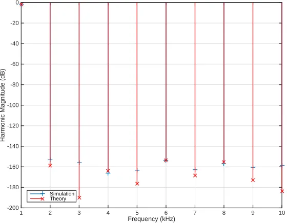
Figure 5: Spectrum of the PWM pulse trainp(t) without ripple compensation: analytical results from (45) and (52),

and numerical results from simulation.

Frequency (kHz)

1 2 3 4 5 6 7 8 9 10

Harmonic Magnitude (dB)

-200 -180 -160 -140 -120 -100 -80 -60 -40 -20 0

Simulation Theory

withu∗= 0.8 andf = 1kHz. For the analytical result in (45), we keep terms atO(1) andO(ǫ); the

output Fourier component at the fundamental frequency is then predicted to be −0.01356−0.4i, while simulation gives −0.0166−0.3988i. The absolute values of the Fourier components for the second, third and fourth harmonics are given in Table 2; further results are summarised in Figure 5. 375

Given the small amplitude of harmonics and the small number of terms kept in the perturbation analysis, these results represent very good agreement between theoretical and numerical results. We note that in a practical implementation any harmonic below about −140dB will disappear beneath the noise floor, and will not be observable in measurement.

In the presence of RC, we may compare simulation results both with the perturbation calcu-380

lation above, and also with the predictions of the small-signal model. Taking terms at O(1) and

O(ǫ), (45) predicts that the output contains only the fundamental. Its prediction of the amplitude of the output fundamental agrees exactly with predictions of the small-signal model, when the latter is appropriately truncated. Whenu(t) is as in (53), withu∗= 0.8 andf = 1kHz, the output

Fourier component at the fundamental frequency is analytically−0.0135−0.3987i, and from sim-385

ulation−0.0166−0.3988i. Further results are summarised in Figure 6; we note that all harmonics beyond the fundamental are beneath the practical noise floor of −140dB. With f instead 2kHz, the corresponding results are −0.0263−0.3949i and −0.0327−0.3952i. At lower amplitude, with

u∗ = 0.5 (and f = 1kHz), the results are −0.0084−0.2492i and −0.0104−0.2492i. Again the

agreement between theoretical prediction and simulation is very good. The largest harmonic in 390

the output is measured to be less than 10−5_{, which confirms the effectiveness of RC in eliminating}

higher harmonics from the output.

7.1. Effects of instability

The bifurcation structure of a negative-feedback pulse-modulated system such as described in this paper can be extremely intricate [5, 6] in response to a sinusoidal reference. However, the 395

practical mode of operation for the present device aims to avoid instability; thus it is sufficient to use an approximation to the stability boundary, as we now describe. From either (26) or (28) we may determine whether the steady-state operating point in response to aconstant inputu0 is

stable or unstable. We find (either with or without RC) that the stability boundary depends only very weakly on the value ofu0. Correspondingly, we find that the steady-state stability threshold

400

-1 -0.5 0 0.5 1

-1 -0.5 0 0.5 1

Figure 7: Path of the eigenvalues of M_{in the complex plane as} c1 is varied from 105/s to 4.5×105/s, all other

parameter values being as in Table 1 and withk= 0. Arrows indicate the direction for increasing values ofc1.

(i.e., one that varies slowly compared with the time scale of the switching). The behaviour of the amplifier is markedly different in the “stable” and “unstable” cases, and in practice the threshold between the cases is quite sharp.

For expository purposes, we use c1 as our bifurcation parameter, holding all other parameters

405

fixed at their values as in Table 1. The paths of the eigenvalues of the matrix M are shown in Figure 7 as c1 is varied from 105/s to 4.5×105/s, for a constant input u0 = 0, with k = 0.

In fact the eigenvalues vary little with the choice of u0 or k. We find that the steady-state

operating point is stable for c1 < c1c, where c1c varies between 2.206×105/s and 2.208×105/s

as u0 varies in the interval [−1,1]. For practical purposes, it is thus a reasonable approximation

410

to consider that there is a single point at which the bifurcation from stability to instability takes place (although a more detailed analysis would undoubtedly reveal a rich, finer-grained bifurcation structure [5, 6]). Instability of the steady-state operating point arises through a pair of complex conjugate eigenvalues ofM leaving the unit circle, as in Figure 7. Beyond the bifurcation point, there are corresponding oscillations in the duty cycle, which grow untilan reaches 0 or 1, at which

415

-6 -5 -4 -3 -2 -1

120000 140000 160000 180000 200000 220000 240000

c

2

3

4

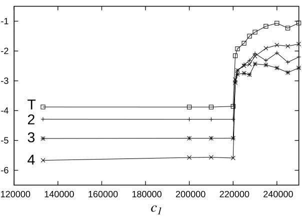
T

Figure 8: Line T shows log10THD as a function of c1, all other parameters being as in Table 1. Lines 2, 3, 4,

respectively, give log10 of the amplitudes of the second, third and fourth harmonics in the output. The input is

u(t) = 0.8 sin(2πf t), withf= 1kHz.

1 lead to a sudden calamitous jump in the amplitude of harmonics in the output, and consequent sudden steep rise in the total harmonic distortion (THD); see Figure 8. The THD of a signal may 420

be defined as follows:

for f(t) =

∞ X

−∞

fneniωt, THD = p

|f2|2_+|f3|2_{+· · ·} |f1| .

As is evident in Figure 8, there appears to be some uncertainty in our measurements of the harmonic amplitudes and the THD beyond the onset of instability, in contrast to our crisp results up to that point. The reason is that, prior to the onset of instability there are just two frequencies in the system, one associated with the audio sine wave and the other associated with the switching. 425

Both frequencies are at our disposal; we choose these two frequencies to be commensurate and ensure that the time interval of simulation is an integer multiple of both the switching period T

and the sine-wave period 1/f. However, beyond the bifurcation point a third frequency is present in the simulations, relating to the oscillations in the duty cycle about the (now unstable) steady-state response. This third frequency arises dynamically in the system and is not a parameter 430

of this oscillation. Consequently, there is spectral leakage [28] (absent before the instability) and our measurements of various harmonic components are correspondingly contaminated. However, beyond the bifurcation point the THD performance of the amplifier is so poor that a precise measurement of the THD is unnecessary: post-instability the amplifier is all but useless for high-435

fidelity reproduction.

Of course our exploration of the high-dimensional parameter space of this amplifier is extremely limited: it is entirely possible that by choosing different parameter values and/or varying different parameters we might find a supercritical bifurcation leading to oscillations that saturate at small amplitude beyond the point of instability. In this case, any rise in THD is likely to be far less 440

dramatic than that observed here.

7.2. Comparison with open-loop design, and experimental results

It is instructive to compare the foregoing results with those from an open-loop design. The latter involves just the carrier-wave generator and comparator from Figure 1, with the audio signal at the positive comparator input and the carrier wave at the negative input. The full output 445

spectrum for the open-loop case is well known [29, 30, 31]: the distortion components in the audio spectrum are due entirely to sidebands of the PWM switching frequency, and are negligible, being smaller than the smallest numerical value that can be represented by Matlab’s floating point 64-bit format. However, despite its extremely low theoretical level of audio distortion, the open-loop design is less advantageous in practice than a closed-loop design, such as examined here, because 450

the latter is considerably better at rejecting unwanted perturbations caused by disturbances to the power supply or other non-idealities of the physical device. Experimental results for a closed-loop class-D amplifier designed by making use of the proposed approach show (see Figure 13 of [32]) that the measured total harmonic distortion (THD) at 1W is equal to 0.3% for the open-loop amplifier and decreases to 0.003% when the feedback loop is closed. Experimental results for a 455

8. Conclusions 460

We have analysed the nonlinear response of a fifth-order pulse-modulated negative-feedback system to a slowly varying input. For the application at hand, we have demonstrated quantitatively the effectiveness of the ripple compensation technique in reducing audio distortion that arises from switching in the negative feedback loop. Our approach complements the usual focus on instability and bifurcation of piecewise-smooth systems [3]; our interest is in the accuracy with 465

which the system tracks its input, which provides a challenging perturbation problem in its own right. We choose system parameters deliberately to be of physical relevance, avoiding instability. Our principal results have been a small-signal model, which linearises about a steady-state point of operation, and a nonlinear perturbation calculation that avoids such a linearisation. While the former is a standard piece of the engineer’s toolkit, the latter, much more powerful, calculation is 470

not.

We emphasise that the techniques described here, particularly the fully nonlinear calculation presented in a quite general formulation in Section 6, are applicable to a wide variety of other nonlinear pulse-modulated systems [4].

Acknowledgments 475

References

[1] M. Berkhout, L. Dooper, Class-D audio amplifiers in mobile applications, IEEE Trans. Circ. Syst. I 57 (2010) 992–1002.

480

[2] H. S. Black, Modulation Theory, Van Nostrand, New York, 1953.

[3] M. Di Bernardo, C. J. Budd, A. R. Champneys, P. Kowalczyk, Piecewise-Smooth Dynam-ical Systems: Theory and Applications, Applied MathematDynam-ical Sciences, vol. 163. Springer, London, 2008.

[4] A. Kh. Gelig, A. N. Churilov, Stability and Oscillations of Nonlinear Pulse-Modulated Sys-485

tems, Birkh¨auser, Boston, 1998.

[5] V. Avrutin, E. Mosekilde, Zh. T. Zhusubaliyev, L. Gardini, Onset of chaos in a single-phase power electronic inverter, Chaos 25 (2015) 043114.

[6] V. Avrutin, Zh. T. Zhusubaliyev, E. Mosekilde, Border collisions inside the stability domain of a fixed point, Physica D 321–322 (2016) 1–15.

490

[7] C. C. Fang, Sampled-Data Analysis and Control of DC–DC Switching Converters, PhD thesis, University of Maryland, College Park, 1997.

[8] S. M. Cox, B. H. Candy, Class-D audio amplifiers with negative feedback, SIAM J. Appl. Math. 66 (2005) 468–488.

[9] S. M. Cox, C. K. Lam, M. T. Tan, A second-order PWM-in/PWM-out class-D audio amplifier, 495

IMA J. Appl. Math. 78 (2013) 159–180.

[10] S. M. Cox, H. du T. Mouton, Ripple compensation for a class-D amplifier, SIAM J. Appl. Math. 75 (2015) 1536–1552.

[11] S. M. Cox, M. T. Tan, J. Yu, A second-order class-D audio amplifier, SIAM J. Appl. Math. 71 (2011) 270–287.

500

[13] T. Mouton, B. Putzeys, Digital control of a PWM switching amplifier with global feedback, in: Audio Engineering Society Conference: 37th International Conference: Class D Audio Amplification, 2009.

505

[14] B. Putzeys, Simple, ultralow-distortion digital pulse width modulator, in: Audio Engineering Society Convention: 120th Convention: Paris, France, 2006.

[15] C. Neesgaard, L. Risbo, PWM amplifier control loops with minimum aliasing distortion. In 120th Audio Engineering Society Convention (2006) Audio Engineering Society.

[16] G. A. Papafotiou, N. I. Margaris, Calculation and stability investigation of periodic steady 510

states of the voltage controlled buck DC–DC converter, IEEE Trans. Power Electr. 19 (2004) 959–970.

[17] M. A. Aizerman, F. R. Gantmakher, On the stability of periodic motions, J. Appl. Math. Mech. 22 (1958) 1065–1078.

[18] C. C. Fang, E. H. Abed, Robust feedback stabilization of limit cycles in PWM DC–DC 515

converters, Nonlinear Dyn. 27 (2002) 295–309.

[19] C. C. Fang, E. H. Abed, Sampled-data modeling and analysis of closed-loop PWM DC–DC converters, in: Proceedings of the IEEE International Symposium on Circuits and Systems, ISCAS ’99, Volume 5, 1999, pp. 110–115.

[20] C. C. Fang, E. H. Abed, Sampled-data modelling and analysis of the power stage of PWM 520

DC–DC converters, Int. J. Electr. 88 (2001) 347–369.

[21] D. A. Harville, Matrix Algebra from a Statistician’s Perspective, Springer, Berlin, 1997. [22] G. Boole, A Treatise On The Calculus of Finite Differences (Second Edition), Macmillan,

London, 1872.

[23] L. M. Milne-Thomson, The Calculus of Finite Differences, Macmillan, London, 1933. 525

[25] J. Yu, M. T. Tan, S. M. Cox, W. L. Goh, Time-domain analysis of intermodulation distortion of closed-loop class-D amplifiers, IEEE Trans. Power Electr. 27 (2012) 2453–2461.

[26] T. M. Apostol, On the Lerch zeta function, Pacific J. Math. 1 (1951) 161–167. 530

[27] M. Di Bernardo, C. K. Tse, Chaos in power electronics: an overview, in: G. Chen, T. Ueta (Eds.) Chaos in Circuits and Systems, World Scientific Series on Nonlinear Science Series B: Volume 11, 2002, pp. 317–340.

[28] F. J. Harris, On the use of windows for harmonic analysis with the discrete Fourier transform, Proc. IEEE 66 (1978) 51–83.

535

[29] D. G. Holmes, T. A. Lipo, Pulse Width Modulation for Power Converters: Principles and Practice. IEEE Press Series on Power Engineering, Vol. 18. John Wiley & Sons, 2003. [30] Z. Song, D. V. Sarwate, The frequency spectrum of pulse width modulated signals, Signal

Proc. 83 (2003) 2227–2258.

[31] S. M. Cox, Voltage and current spectra for a single-phase voltage-source inverter, IMA J. 540

Appl. Math. 74 (2009) 782–805.

[32] P. Kemp, T. Mouton, B. Putzeys, High-order analog control of a clocked class-D audio am-plifier with global feedback using z-domain methods. In 131st Audio Engineering Society Convention (2011) Audio Engineering Society.

[33] P. J. Kemp, High-order analog control of a clocked class-D audio amplifier with global feedback 545