Accretion discs as regulators of stellar angular momentum evolution in
the ONC and Taurus–Auriga
Claire L. Davies,
‹Scott G. Gregory and Jane S. Greaves
SUPA School of Physics and Astronomy, University of St Andrews, North Haugh, St Andrews, Fife KY16 9SS, UK
Accepted 2014 July 23. Received 2014 July 22; in original form 2014 April 8
A B S T R A C T
In light of recent substantial updates to spectral type estimations and newly established intrinsic colours, effective temperatures, and bolometric corrections for pre-main sequence (PMS) stars, we re-address the theory of accretion disc-regulated stellar angular momentum (AM) evolution. We report on the compilation of a consistent sample of fully convective stars within two of the most well-studied and youngest, nearby regions of star formation: the Orion nebula Cluster and Taurus–Auriga. We calculate the average specific stellar AM (j) assuming solid body rotation, using surface rotation periods gathered from the literature and new estimates of stellar radii and ages. We use publishedSpitzerIRAC fluxes to classify our stars as Class II or Class III and compare theirjevolution. Our results suggest that disc dispersal is a rapid process that occurs at a variety of ages. We find a consistentjreduction rate between the Class II and Class III PMS stars which we interpret as indicating a period of accretion disc-regulated AM evolution followed by near-constant AM evolution once the disc has dissipated. Furthermore, assuming our observed spread in stellar ages is real, we find that the removal rate ofjduring the Class II phase is more rapid than expected by contraction at constant stellar rotation rate. A much more efficient process of AM removal must exist, most likely in the form of an accretion-driven stellar wind or other outflow from the star–disc interaction region or extended disc surface.
Key words: accretion, accretion discs – stars: formation – stars: late-type – stars: pre-main-sequence – stars: rotation – stars: variables: T Tauri, Herbig Ae/Be.
1 I N T R O D U C T I O N
If all angular momentum (AM) was conserved during contrac-tion from a natal molecular cloud to the zero-age main sequence (ZAMS), stellar rotational velocities would far exceed those re-quired to break a star apart. A solar mass star, accreting at a typical rate of 10−7M
yr−1would reach its break-up velocity after just
1 Myr (Hartmann & Stauffer1989). However, stars with accretion discs are found to be rotating at much slower rates, suggesting that significant AM removal mechanisms must operate during the first few Myr of formation (Bouvier et al.1986; Hartmann et al.1986). Accretion disc-regulated AM removal was initially attributed to a magnetic torque produced by the differential rotation between a star and its Keplerian disc (Ghosh & Lamb1979; Camenzind1990; K¨onigl1991; Collier Cameron & Campbell1993). For this torque to sufficiently break the star, the stellar magnetic field would need to interact with a region in the disc beyond the corotation radius and be stable over multiple rotations. However, differential twisting of the magnetic field lines, together with the competing processes of
E-mail:[email protected]
accretion and diffusion, limit the size of the connected region in the disc and reduce the extent of the field beyond corotation (Shu et al. 1994; Bardou & Heyvaerts1996; Agapitou & Papaloizou2000; Matt & Pudritz2005; Zanni & Ferreira2009). Thus, such a mecha-nism would be insufficient to spin down the star. These findings have prompted more recent theoretical studies to favour star–disc interac-tion related magnetized winds and outflows as possible AM removal mechanisms in actively accreting pre-main sequence (PMS) stars (Shu et al.1994; Lovelace, Romanova & Bisnovatyi-Kogan1995; Matt & Pudritz2005; Zanni & Ferreira2013).
Observational studies of AM evolution in PMS stars primarily focused on the distribution of stellar surface rotation rates. Until the formation of a radiative core, stellar rotation can be approx-imated to that of a solid body. Therefore, while the PMS star is fully convective, the surface rotation period can be used to study the AM of the entire star. In young star-forming regions, such as the Orion nebula Cluster (ONC), NGC 2264, IC 348, and Taurus– Auriga, distributions of PMS surface rotation periods were observed to be bimodal (e.g. Attridge & Herbst1992; Edwards et al.1993; Choi & Herbst1996; Herbst et al.2000; Cohen, Herbst & Williams 2004; Herbst & Mundt2005; Lamm et al.2005; Cieza & Baliber 2007) with the peak of slower rotators interpreted as indicating
2014 The Authors
at University of St Andrews on December 8, 2014
http://mnras.oxfordjournals.org/
disc-regulated AM removal. Once the disc dissipates, the star con-serves AM, spinning up as it contracts, and is observed in the peak of more rapid rotators.
Accretion disc-regulated PMS AM evolution has not found unan-imous support. Certain studies have not observed a relationship be-tween stellar rotation and accretion disc indicators. However, these contrasting findings can be explained in terms of a variety of biases, masking the underlying relationship between accretion and rota-tion. For instance, early studies of PMS rotation rates were affected by aliasing and beat phenomena (e.g. Stassun et al.1999), inclu-sion of non-members (e.g. Rebull 2001), and unreliable indica-tors of accretion discs (e.g. Makidon et al. 2004). Furthermore, an underlying relationship between rotation rate and stellar mass has been uncovered (Herbst et al. 2002; Cieza & Baliber2007), used to explain the more unimodal rotation period distributions seen in some studies (e.g. Stassun et al. 1999). This mass ef-fect is partially attributable to the comparative sizes of ‘high’ and ‘low’ mass stars. For a sample of stars of a given age and spe-cific stellar AM, j, those with lower masses will have smaller radii,R. Sincej∝R2
/P, the rotation periods, P, of the lower
mass sample will be shorter than the higher mass sample (Herbst, Bailer-Jones & Mundt2001). Thus, the lower mass slow rotators are shifted towards the peak of rapid rotators, blurring the bimodal-ity found for the higher mass sample.
Cieza & Baliber (2007) found the bimodality of the rotation period distributions to be severely affected by even a small contam-ination of stars with spectral types later than M2. The difference in size between the higher and lower mass stars cannot explain this alone and the location of this boundary remains poorly under-stood. The most promising underlying physical explanation relates to changes in the strength and geometry of the large-scale stellar magnetic field around this spectral type (Lamm et al.2005).
The efficiency of AM removal via magnetized winds or out-flows is related to the relative strength of the dipole compo-nent of the magnetic field as this governs the position of the disc truncation radius and the level of flux from open mag-netic fields (Gregory et al. 2008; Adams & Gregory 2012; Johnstone et al. 2014). Donati et al. (2011) found this mech-anism to be most efficient in PMS stars of ∼0.5–1.3 M. The growth of a radiative core in higher mass stars inhibits the build-up of a strong dipole field (Donati et al. 2011) and lower mass stars, although still fully convective, appear to have weaker large-scale magnetic fields (Donati et al. 2010, 2013; Gregory et al. 2012). Thus, the magnetic fields of stars later than M2 truncate their discs closer to the star, meaning they rotate more rapidly than their higher mass, fully convective counterparts. Although less efficient for lower mass stars, ac-cretion disc regulation can still explain their AM evolution during the first few Myr (Rodr´ıguez-Ledesma, Mundt & Eisl¨offel 2010; Irwin et al.2011).
In this paper, we focus on the evolution of specific stellar AM (j) in two of the youngest, nearby regions of star formation, namely the ONC (∼1 Myr; Hillenbrand1997) and Taurus–Auriga (∼2.8 Myr; White & Ghez2001). The well-studied nature and youthful ages of these two regions allows us to split the sample according to their position in the Hertzsprung–Russel (HR) diagram into fully convective and partially convective samples. In Section 2, we sum-marize the model used to calculate j and how we determined which stars are fully convective. Section 3 details how the data required to calculatejwere obtained and how we split our data into ‘high mass’ and ‘low mass’ samples. Our results are detailed in Section 4 and summarized in Section 5.
2 A N G U L A R M O M E N T U M M O D E L
The AM of a rotating object is a product of its moment of inertia and angular velocity. Thus, in order to calculate the stellar AM, we need to be able to model the distribution and rotation of stellar material. This calculation is greatly simplified for low mass PMS stars as they are fully convective during at least the first few Myr of contraction (Limber1958; Chabrier & Baraffe1997; Gregory et al.2012). Thus, they lack the layer of high rotational velocity sheer that exists at the boundary between the radiative core and convective envelope in partially convective stars like the Sun, and generates surface differential rotation.
Studying the levels of differential rotation present on stellar sur-faces is possible with tomographic Doppler imaging techniques. This requires spectroscopic monitoring of stars over a few rotations and with sufficient phase coverage. As this is telescope time inten-sive, to date the surface differential rotation rate, d, has only been measured for a handful of fully convective PMS stars. The fully convective, non-accreting PMS stars, TWA 6, LkCa 4, and V410 Tau each have differential rotation rates consistent with solid body rotation (d=0) to within 1.7σ(Skelly et al.2008,2010; Carroll et al.2012; Donati et al.2014). However, Donati et al. (2010) found that the fully convective accreting PMS star V2247 Oph exhibited substantial differential rotation with d=0.32±0.05 rad d−1. To
date, this is the only fully convective PMS star with measured sur-face differential rotation. It is also the lowest mass star of the sample and has a large-scale magnetic field that is more complex than that of higher mass fully convective PMS stars. It may exist in a regime of dynamo bistability, whereby stars with otherwise similar param-eters have drastically different large-scale magnetic topologies and surface differential rates, as has been found for the lowest mass main-sequence (MS) M dwarfs (cf. Gregory et al.2012). Further observations are required to determine how common differential rotation like that observed in V2247 Oph is.
For now, we assume that the surfaces of fully convective PMS stars rotate as solid bodies (the usual assumption of stellar evolution models; e.g. Eggenberger et al.2012). This is consistent with the observations of TWA 6, LkCa 4, and V410 Tau, as well as the observational study of Barnes et al. (2005) who found a decrease in surface differential rotation with increasing convective zone depth. Solid body rotation is also typically found in numerical models (e.g. Kuker & Rudiger1997) and magnetohydrodynamic simulations (e.g. Browning2008) of fully convective stars.
For a fully convective star of mass,M, and radius,R, rotating with angular velocity,=2π/P, the specific stellar AM is then given by
j= MJ
=
2πk2R2
P , (1)
whereJis the stellar AM,Pis the rotation period, andkis the radius of gyration (Chandrasekhar & M¨unch1950; Krishnamurthi et al. 1997; Herbst & Mundt2005). For a perfect sphere,k2 =(2/3).
However, the most rapidly rotating stars in our sample will be distorted from a spherical shape. To account for this, we explicitly calculate the radius of gyration for each individual star. Following Herbst & Mundt (2005),
k2=
4 3a
4+16
15a
3b+8
7a
2b2+ 16
105ab
3+ 52
1155b
4
×
2a2+2
5b
2
−1
, (2)
at University of St Andrews on December 8, 2014
http://mnras.oxfordjournals.org/
where if we model a PMS star as a polytrope of index,n=3/2,
a=1.74225ν+1 (3)
and
b=3.86184ν. (4)
Here,
ν= 2π
GP2ρ c
, (5)
whereGis the gravitational constant andρcis the central density
of the star (Chandrasekhar1935).
Equation (1) is valid for each star until it forms a radiative core. The age at which this happens is dependent on the stellar mass. Stars below∼0.35 Mremain fully convective throughout their formation and during their MS lifetimes (Limber1958; Chabrier & Baraffe1997). More massive stars form radiative cores during their contraction. Gregory et al. (2012) derived the mass-dependent age at which a star of mass greater than 0.35 Mwould develop a radiative core where
tcore≈
1.494M M
2.364
Myr (6)
based on Siess, Dufour & Forestini (2000) PMS evolutionary mod-els. Accordingly, we limit our analysis to stars with isochronal ages (Section 3.3) below their individualtcorelimit.
3 S T E L L A R DATA
In order to calculatejusing equation (1) and study its evolution for fully convective stars in the ONC and Taurus–Auriga, we required estimates of stellar masses, radii, central densities, ages, and rotation rates as well as reliable indicators of accretion disc presence. Both the ONC and Taurus–Auriga have well-studied stellar populations (e.g. Hillenbrand1997; Luhman et al.2010) but a range of different methods have been adopted to calculate their properties. In the ma-jority of cases, estimates of stellar masses and ages have relied on the comparison of observationally derived effective temperatures,Teff,
and bolometric luminosities,L, or colour–magnitude diagrams, to theoretical PMS evolutionary models. However, the choice of PMS evolutionary model differs between studies and multiple methods have been employed to translate spectral types and optical magni-tudes intoTeffandL.
To compare our findings for the ONC with those of Taurus– Auriga, it was necessary to assignTeffand calculateLin a fully
consistent manner. We gathered spectral types and optical magni-tudes from the literature, as detailed below. We adopt the recently derived scales of Pecaut & Mamajek (2013) which account for the bluer colours of PMS stars by accounting for the combined effects of their lower surface gravities (Luhman1999; Da Rio et al.2010; Pecaut & Mamajek2013; Herczeg & Hillenbrand2014) and spot-ted surfaces (Gullbring et al.1998; Stauffer et al.2003) and are thus more applicable here than typically used MS dwarf scales (e.g. Bessell & Brett1988; Bessell1995; Kenyon & Hartmann 1995; Luhman1999). Details of this process are presented in Sections 3.1 and 3.2. We calculate stellar radii using our values ofTeffandLand
adopt the Siess et al. (2000) PMS evolutionary models to translate
TeffandLinto stellar masses and ages. Details of these processes
are outlined in Sections 3.3 and 3.4.
For the stellar rotation rates, we gathered previously determined rotation periods from the literature. By using rotation periods rather than projected rotational velocities,vsini, we removed the depen-dence on unknown stellar inclinations. The sources of rotational period data used, as well as the checks we employed to ensure that we avoided previously reported sources of bias, are presented in Section 3.5.
To study the dependence of AM evolution on the presence of an accretion disc, we identified all Class II and Class III PMS stars in our ONC and Taurus–Auriga samples. The details of this process are outlined in Section 3.6.
The compiled data sets for the ONC and Taurus–Auriga are pre-sented in Tables1and2, respectively. These tables include all mem-bers (Section 3.5.2) for which a spectral type was available that had not previously been identified as a binary or multiple system (Sec-tion 3.2.1). Stars found not to be fully convective (Sec(Sec-tion 2) were removed from the analysis but are included in Tables1and2for completeness.
3.1 Effective temperatures
Spectroscopically determined spectral types were gathered from the literature. Tables1and2list the individual reference for each star in our ONC and Taurus–Auriga samples, respectively. For the bulk of ONC stars, spectral types were retrieved from the newly updated cluster census of Hillenbrand, Hoffer & Herczeg (2013, hereafter H13). Where multiple spectral types were retrieved for the same star, good agreement was found in general but, in the instances where studies had determined different spectral types, preference was given to the most recent studies.
A number of very low mass stars in the ONC did not have spec-troscopically determined spectral types available in the literature. However, some of these did have spectral types calculated using the 7770 Å narrow-band filter in Da Rio et al. (2010). In a recent study, Hillenbrand et al. (2013) found a seemingly large scatter between these photometrically determined spectral types and those deter-mined spectroscopically. However, they also noted that their newly determined spectral types for the lowest mass stars also displayed a similar level of scatter compared to previous spectral types. With this in mind, we adopt these photometrically determined spectral types for the very low mass stars with no spectroscopically deter-mined spectral types.
We made use of newly derived spectral type-to-Teffconversions
for 5–30 Myr old PMS stars detailed in table 6 of Pecaut & Mamajek (2013). Although both the ONC and Taurus–Auriga are younger than 5 Myr, these effective temperatures are more applicable than the typically used MS dwarf scales (e.g. Bessell & Brett 1988; Bessell1995; Kenyon & Hartmann1995; Luhman1999) as they take into account the lower surface gravities and the presence of cool starspots on the surfaces of PMS stars (Gullbring et al.1998; Luhman1999; Stauffer et al.2003; Da Rio et al.2010; Pecaut & Mamajek2013; Herczeg & Hillenbrand2014). However, they are only available for stars of spectral type F0 to M5. This has little effect on our results as most stars later than M5 have masses below 0.1 Mand therefore fall below the lowest mass track in the Siess et al. (2000) models (which we adopt to estimate stellar masses and ages, see Section 3.3) and stars of spectral types earlier than F0 are too massive to be T Tauri stars. For the seven stars in our sample with spectral types later than M5, the spectral type-to-Teff
conversions for MS dwarfs detailed in table 5 of Pecaut & Mamajek (2013) were adopted for continuity.
at University of St Andrews on December 8, 2014
http://mnras.oxfordjournals.org/
Table 1. Stellar data for all members of the ONC not identified as binary or multiple for which a spectral type was available in the literature (see Section 3.5.2 for membership constraints). The full table is available in electronic form in the supporting information section. A sample is given here to illustrate its content. Column 1 gives the SIMBAD identification for the star; columns 2, 3, and 4 list the adopted spectral type (SpT), its error in spectral subtype, and the reference as in Hillenbrand et al. (2013,H13) [except (D10) – Da Rio et al.2010]; columns 5 and 6 list the effective temperature,Teff, and logarithmic bolometric luminosity,
log (L/L), calculated from SpT and optical photometry (see Sections 3.1 and 3.2 for details); columns 7 and 8 list the stellar mass in solar units and the age in Myr, respectively, calculated fromTeffand log (L/L) using Siess et al. (2000) PMS evolutionary models (see Section 3.3); column 9 lists the stellar radius in solar units; columns 10, 11, and 12 list the adopted rotation period in days, the observed waveband for rotation period measurement (opt – optical, NIR – near infrared, MIR – mid infrared), and the reference for the rotation period (E93 – Edwards et al.1993, G95 – Gagne, Caillault & Stauffer1995, C96 – Choi & Herbst1996, S99 – Stassun et al.1999, H00 – Herbst et al.2000, C01 – Carpenter et al.2001, Re01 – Rebull2001, Rh01 – Rhode, Herbst & Mathieu2001, H02 – Herbst et al.2002, F09 – Frasca et al.2009, P09 – Parihar et al.2009, R09 – Rodr´ıguez-Ledesma et al.2009, and M11 – Morales-Calder´on et al.2011); columns 13 and 14 list the source classification based on MIR excess measurements (II – disced, III – discless), and based on the EW (CaII) (A – accreting,
N – not accreting) as detailed in Sections 3.6 and 4.2, respectively; column 15 lists the reason, where applicable, for a star’s exclusion from the final analysis [a – not fully convective (see equation 6 and Section 2), b – star lies outside the limits imposed in isochronal fitting (see Section 3.3), c – no optical photometry available to calculateL(see Section 3.2), d –P>15 d (see Section 3.5), e –j>jcrit(see Section 3.5), f – no reliable rotation period available, and g – able
to calculatejbut not able to classify source as II or III].
SIMBAD SpT σ(SpT) Ref. Teff log (L/L) M Age R Period Obs Ref. Class Accretion Notes
(K) M (Myr) R (d)
(1) (2) (3) (4) (5) (6) (7) (8) (9) (10) (11) (12) (13) (14) (15)
LT Ori G8 1 Ste 5210 1.128 2.73−+00..2721 1.80+−00..6050 4.49±0.54 0.50 opt G95 – – a, e V1229 Ori K0 1 H 5030 1.119 2.86−+00..1318 1.20+−00..5030 4.77±0.58 14.30 opt H00 III – a V1963 Ori G8 1 H 5210 1.004 2.53−+00..2228 2.20+−00..9060 3.90±0.47 3.37 MIR M11 III N a V2235 Ori K1 1 H 4920 0.917 2.47−+00..2027 1.40+−00..8050 3.96±0.52 17.91 opt H02 II A a, d V403 Ori K3 1 H 4550 1.357 2.51−+01..4902 0.30+−00..1010 7.68±1.15 6.09 MIR M11 III N a
AK Ori K2 1 Ste 4760 0.89 2.21−+00..3449 1.00+−00..8040 4.09±0.59 10.33 opt G95 II – a V1232 Ori G6 1 H 5390 0.914 2.20−+00..1425 3.70+−10..5090 3.28±0.40 1.55 opt H00 III N a V1509 Ori K2.5 1 H 4655 1.011 2.11−+00..5259 0.60+−00..4020 4.92±0.71 6.99 opt R09 III N a V426 Ori K2 1 H 4760 0.935 2.26−+00..3457 0.90+−00..7040 4.31±0.62 5.15 opt H02 II N a AF Ori G8 3 H13 5210 0.698 2.00−+00..2330 4.20+−32..4000 2.74±0.44 – – – II A a, f KM Ori K3 1 Ste 4550 1.143 2.08−+00..5785 0.40+−00..2020 6.00±0.90 17.40 opt H00 III – d V348 Ori K3 1 Ste 4550 0.964 1.76−+00..6359 0.50+−00..4020 4.88±0.73 8.71 opt H00 II N – V1331 Ori K3e 1 Sta 4550 0.854 1.65−+00..5849 0.60+−00..5020 4.30±0.65 10.70 opt H00 – N g V1444 Ori K3 1 Ste 4550 0.79 1.63−+00..4951 0.70+−00..6030 4.00±0.60 3.45 opt H00 III – – V2299 Ori K3 1 Ste 4550 0.808 1.66−+00..4851 0.70+−00..6030 4.08±0.61 – – – II N f V1294 Ori K3 1 Ste 4550 0.83 1.60−+00..5741 0.60+−00..6020 4.18±0.63 6.76 opt H00 III – – V1333 Ori K3 1 Ste 4550 0.601 1.54−+00..4045 1.10+−10..1050 3.21±0.48 9.23 opt H00 – N a V2140 Ori K2 1 H 4760 0.296 1.58−+00..1212 4.30+−31..2090 2.06±0.30 3.82 opt H02 – N a V401 Ori K2 1 H 4760 0.228 1.51−+00..1113 5.50+−32..7060 1.91±0.28 6.63 opt S99 II – a V356 Ori K3 1 Ste 4550 0.403 1.44−+00..2937 1.80+−20..0080 2.56±0.38 1.57 opt H00 – N a V494 Ori K3 1 H 4550 0.396 1.46−+00..2740 1.90+−10..9090 2.54±0.38 – – – II – a, f AC Ori K3.5 3 LR 4450.5 0.605 1.30−+00..7669 0.80+−20..6040 3.38±0.88 – – – – A f
MU Ori K3 1 Ste 4550 0.001 1.28−+00..0917 6.90+ 5.10
−3.60 1.61±0.24 2.22 opt H02 III N a
AE Ori K4 1 Ste 4330 1.201 1.26−+00..9120 0.20+−00..1017 7.10±1.09 3.42 opt H00 III N – V1330 Ori K4 1 H 4330 0.71 1.15−+00..4035 0.50+−00..3010 4.03±0.62 8.67 opt H00 III – – V1337 Ori K0 2 H 5030 0.02 1.14−+00..1911 17.50+−98..5000 1.34±0.21 – – – II N a, f LU Ori K4 1 Ste 4330 0.687 1.11−+00..4833 0.50+−00..4010 3.93±0.60 4.08 opt H00 III – – V1397 Ori K2 1 H 4760 −0.127 1.11+−00..1313 16.00+−106.60.00 1.27±0.18 5.41 opt H00 – – a V377 Ori K4 1 Ste 4330 0.36 1.11−+00..3632 1.20+−10..1050 2.70±0.41 13.00 opt H02 III – –
Where individual errors on spectral types were not published, an estimate of±1 spectral subtype was adopted. Where a range of possible spectral types was quoted from a single source for a particular star, the median spectral type of the published range was adopted. In this case, the error on the spectral type was adjusted to account for the increased range of possible values. For instance, a star with a published value of spectral type given as K2–K7 would be assigned a spectral type of K4.5 and an error of ±2 spectral subtypes.
3.2 Bolometric luminosities
L can be calculated from the application of a bolometric correc-tion to a single distance modulus- and extinccorrec-tion-corrected optical apparent magnitude (Hillenbrand1997). However, the choice of waveband is crucial in order to ensure that only photospheric emis-sion is observed. For Class II objects,U- andB-band magnitudes are unsuitable as they contain additional emission resulting from accretion. Similarly,J,H, andKbands are unsuitable as they can
at University of St Andrews on December 8, 2014
http://mnras.oxfordjournals.org/
Table 2. Stellar data for all members of Taurus–Auriga not identified as binary or multiple for which a spectral type was available in the literature. The full table is available in electronic form in the supporting information section. A sample is given here to illustrate its content. Column 1 gives the SIMBAD identification for the star; columns 2 and 3 list the SpT and its error in spectral subtype; column 4 lists the effective temperature,Teff, calculated from SpT (see
Section 3.1 for details); columns 5 and 6 list the observedV-band magnitude and (B−V) colour; columns 7 and 8 list the observedIcmagnitude and (V−Ic)
colour; column 9 lists the adopted logarithmic bolometric luminosity, log (L/L) (see Section 3.2 for details); columns 10 and 11 list the stellar mass in solar units and the age in Myr, estimated fromTeffand log (L/L) using Siess et al. (2000) PMS evolutionary models (see Section 3.3 for details); column 12 lists the stellar radius in solar units; column 13 lists the rotation period in days; column 14 lists the classification of the object based on SED fitting (II – disced, III – discless; see Section 3.6 for details); column 15 lists the references for the SpT, photometry, rotation period, and source classification [(1) – Cohen & Kuhi 1979, (2) – Bouvier et al.1986, (3) – Herbst & Koret1988, (4) – Beckwith et al.1990, (5) – Bouvier1990, (6) – Bouvier et al.1993, (7) – Edwards et al.1993, (8) – Grankin1993, (9) – Herbst et al.1994, (10) – Strom & Strom1994, (11) – Kenyon & Hartmann1995, (12) – Fernandez & Eiroa1996, (13) – Grankin 1996, (14) – Osterloh, Thommes & Kania1996, (15) – Wichmann et al.1996, (16) – Bouvier et al.1997, (17) – Grankin1997, (18) – Brice˜no et al.1998, (19) – Luhman & Rieke1998, (20) – Brice˜no et al.1999, (21) – Wichmann et al.2000, (22) – Mora et al.2001, (23) – Roberge et al.2001, (24) – Stassun et al. 2001, (25) – White & Ghez2001, (26) – Brice˜no et al.2002, (27) – Vieira et al.2003, (28) – Luhman2004, (29) – Andrews & Williams2005, (30) – Massarotti et al.2005, (31) – Broeg et al.2006, (32) – Kundurthy et al.2006, (33) – Padgett et al.2006, (34) – Scholz, Jayawardhana & Wood2006, (35) – Xing, Zhang & Wei2006, (36) – Grosso et al.2007, (37) – Chapillon et al.2008, (38) – Grankin et al.2008, (39) – Luhman et al.2009, (40) – Espaillat et al.2010, (41) – Luhman et al.2010, (42) – Rebull et al.2010, (43) – Andrews et al.2011, (44) – Furlan et al.2011, (45) – Xiao et al.2012, (46) – Cody et al.2013, and (47) – Grankin2013]; column 16 lists the reason, where applicable, for a star’s exclusion from the final analysis [a – not fully convective (see equation 6 and Section 2), b – star lies outside the limits imposed in isochronal fitting (see Section 3.3), c – no optical photometry available to calculateL(see Section 3.2), d –P>15 d (see Section 3.5), e –j>jcrit(see Section 3.5), f – no reliable rotation period available, and g – able to calculatejbut not able to classify source as II or III].
SIMBAD SpT σ(SpT) Teff V B−V Ic V−Ic log (L) M Age R Period Class Refs. Notes
(K) L M (Myr) R (d)
(1) (2) (3) (4) (5) (6) (7) (8) (9) (10) (11) (12) (13) (14) (15) (16)
HD 282600 K2 1 4760 10.72 1.62 – – 0.943 2.28+−00..5734 0.90−+00..7040 4.36±0.63 – – 21 a, f
HD 282624 G8 2 5210 9.15 0.89 8.10 1.05 0.823 2.21+−00..2521 3.10−+11..8000 3.16±0.42 2.661 II 30, 11, 46, 41 a RY Tau K1 1 4920 10.22 1.03 8.80 1.42 0.729 2.16+−00..1615 2.10−+01..3080 3.19±0.42 5.6 II 41, 11, 3, 29, 42 a
HD 283572 G5 1 5500 9.03 0.81 8.10 0.93 0.824 1.98+−00..2519 5.00−+12..6020 2.84±0.35 1.55 III 42, 11, 5, 41 a HD 283782 K1 2 4920 9.62 0.84 8.58 1.04 0.580 1.95+−00..1513 3.10−+11..4010 2.68±0.34 – – 15, 21 a, f HD 30171 G5 1 5500 9.26 0.75 8.36 0.9 0.702 1.74+−00..1723 7.10−+22..4020 2.47±0.30 1.104 III 16, 21, 47, 41 a HD 285281 K1 2 4920 12.03 0.94 9.69 1.09 0.395 1.69+−00..1514 4.90−+12..1060 2.17±0.27 1.1683 – 15, 21, 47 a, g GM Aur K3 1 4550 10.21 1.19 9.12 2.34 0.872 1.69+−00..5353 0.60−+00..5020 4.39±0.66 12 II 25, 11, 24, 41 – HD 286178 K1 2 4920 10.30 0.95 9.13 1.08 0.385 1.68+−00..1513 4.90−+12..4060 2.14±0.27 1.72 – 15, 21, 33, 47 a, g HD 283641 K0 2 5030 11.34 1.32 – – 0.408 1.67+−00..1615 5.70−+12..3050 2.11±0.25 – – 15, 47 a, f V1110 Tau K0 1 5030 10.09 0.89 – – 0.376 1.62+−00..1616 6.30−+12..7070 2.03±0.25 3.039 III 42, 38, 47, 29 a V1298 Tau K1 2 4920 10.38 0.88 9.36 1.02 0.256 1.51+−00..1713 6.90−+23..6020 1.85±0.23 2.86 – 15, 21, 47 a, g HD 285957 K1 2 4920 10.72 0.93 9.60 1.12 0.222 1.46+−00..1514 7.70−+23..3060 1.78±0.22 3.0789 – 15, 21, 47 a, g HD 282630 K0 2 5030 10.85 1.02 9.68 1.17 0.232 1.43+−00..1714 8.90−+24..6020 1.72±0.21 2.2393 III 15, 11, 46, 41 a HD 281691 K1 2 4920 10.65 0.85 9.60 1.05 0.178 1.41+−00..1613 8.60−+23..9070 1.69±0.21 2.662 – 15, 21, 47 a, g HD 31281 G1 2 5970 9.22 0.62 – – 0.571 1.37+−00..0710 15.00−+33..5000 1.80±0.21 – – 15, 47 a, f V1299 Tau G3 2 5740 9.33 0.61 8.61 0.72 0.506 1.36+−00..0914 14.00−+34..0050 1.81±0.22 0.816 – 15, 21, 47 a, g V1072 Tau K0 2 5030 10.34 0.79 9.45 0.89 0.174 1.34+−00..1316 10.50−+25..0080 1.61±0.19 2.74 III 15, 11, 24, 29 a V1319 Tau G8 2 5210 10.26 0.65 9.38 0.88 0.205 1.30+−00..1613 13.00−+36..5030 1.55±0.18 0.736 – 15, 21, 47 a, g V1079 Tau K3 1 4550 12.41 1.37 10.79 1.62 −0.018 1.26+−00..1809 7.00−+36..0050 1.58±0.24 5.85 II 40, 11, 32, 41 a
HD 284266 K0 2 5030 10.56 0.73 9.68 0.88 0.082 1.23+−00..1215 13.50−+36..5080 1.45±0.17 1.812 – 15, 21, 47 a, g CW Tau K3 1 4550 13.34 1.37 11.42 1.92 −0.083 1.21+−00..1109 9.00−+47..0050 1.46±0.22 8.2 II 11, 32, 41 a HD 285840 K1 2 4920 10.81 0.82 – – 0.022 1.21+−00..1414 13.50−+48..0030 1.41±0.18 1.561 – 15, 47 a, g HD 285372 K3 2 4550 11.69 1.07 10.43 1.26 −0.098 1.20+−00..1108 9.50−+46..5010 1.44±0.20 0.574 – 15, 21, 31 a, g HD 284496 K0 2 5030 10.81 0.83 – – 0.015 1.14+−00..1115 17.50−+67..0050 1.34±0.16 2.7136 – 15, 38, 47 a, g
contain excess emission from dust. We follow Hillenbrand (1997) and use CousinsIc-band photometry to calculateL, ensuring that
both accretion and disc emission remain minimal.
As in Hillenbrand (1997), we calculate luminosities from the observed photometry,
log
L
L
=0.4[Mbol, −(Ic−AIc)+DM
−BCIc(Teff)]. (7)
Here,Mbol, =4.755 mag is the bolometric absolute magnitude of
the Sun (Mamajek2012),1I
cis the apparent magnitude of emission
in the CousinsIcband,AIcis the extinction atIc,DMis the distance
1We consistently use physical constants and solar values from Eric
Mamajek’s ‘Basic Astronomical Data for the Sun’ (http://sites.google.com/ site/mamajeksstarnotes/basic-astronomical-data-for-the-sun) throughout this study.
at University of St Andrews on December 8, 2014
http://mnras.oxfordjournals.org/
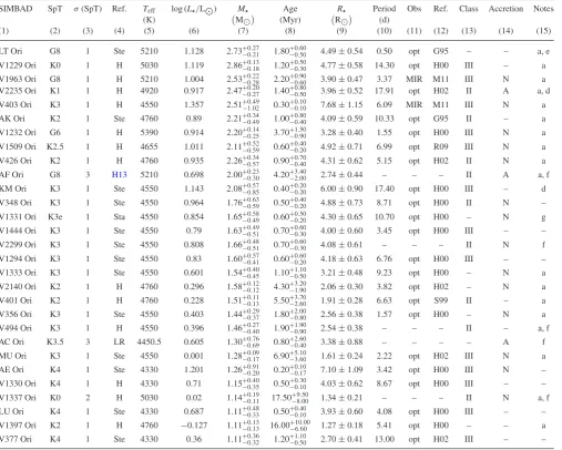
Figure 1. Comparison between newly calculated luminosities for our ONC sample and those of Hillenbrand (1997), adjusted to account for the different distance modulus and solar bolometric luminosity used in this study. The dashed line shows a one-to-one fit to the data. In general, good agreement is found. The main source of spread is caused by the use of different spectral types.
modulus, andBCIc(Teff) is the temperature-dependent bolometric
correction atIc.
We used spectral type-dependent intrinsic colours, (V−Ic)0, and V-band bolometric corrections,BCV(Teff), presented in Pecaut &
Mamajek (2013, see Section 3.1 for the reasoning behind the use of these models), to derive individual values ofBCIc(Teff) such that
BCIc(Teff)=BCV(Teff)+(V −Ic)0. (8) We adopt the extinction law of Rieke & Lebofsky (1985), trans-formed from the Johnsons to the Cousins photometric system by Hillenbrand (1997),
AIc =0.61AV=1.56[(V−Ic)−(V−Ic)0], (9)
where (V−Ic)0is the intrinsic colour appropriate to the spectral
type of the star and (V−Ic) is the observed value. In the case where
negative values of extinction were calculated, this indicated that the observed colours of that star were too blue for the assigned spectral type. For these stars,AIcwas set equal to zero. Consequently, the
Lcalculated for these stars are lower limits and are considered as such in the following analysis.
The distance modulus is assumed to be constant for all stars within each star-forming region. For the ONC, we adopt a distance of 414± 7 pc (Menten et al.2007) and, for Taurus–Auriga, we adopt 140±20 pc (Elias1978; Loinard et al.2007; Torres et al. 2009,2012).
V- and Ic-band photometry for the ONC was taken from
Hil-lenbrand (1997). Fig. 1 compares the new L for our ONC sample against theLfrom Hillenbrand (1997), adjusted to account for the different distance modulus and solar bolometric magnitude we have used. In the majority of cases, our updatedLagree well with those in Hillenbrand (1997). The main source of spread can be attributed to our usage of updated spectral types.
For the Taurus–Auriga region, individual sources ofV- andIc
-band photometry are detailed in Table2. Due to the periodic nature
of the stars in our sample (Section 3.5), only data from studies that took contemporaneous measurements in both wavebands were in-cluded. The number of members of the Taurus–Auriga star-forming region (∼348; Luhman et al.2010) is much smaller than that of the ONC (>1000; Da Rio et al.2010) and the region has higher levels of optical extinction. These differences mean that the Taurus–Auriga sample is much smaller than the ONC sample. To attempt to counter this, we also obtainedB- andV-band photometry which enabled us to calculateL fromV-band magnitudes for additional 23 stars in Taurus–Auriga. In this case,
log L
L
=0.4[Mbol, −(V−AV)+DM
−BCV(Teff)], (10)
where the extinction atVis taken from Rieke & Lebofsky (1985) such that
AV=3.09[(B−V)−(B−V)0]. (11)
Here, (B− V)0is the intrinsic (B− V) colour, again taken from
Pecaut & Mamajek (2013).
Our choice of waveband should reduce the level of contamina-tion by sources other than pure photospheric emission. However, as we make no attempt to calculate the accretion luminosity for any of the stars in our sample, ourL may be underestimated for the most active accretors due to underestimated extinction values (Hillenbrand1997; Da Rio et al.2010). Additionally, our method may lead to the underestimation ofLfor stars hosting dense discs at high inclinations (Kraus & Hillenbrand2009). We attempt to take both of these effects into account by assuming a conservative error estimate of±0.1 dex in logL/Lfor all stars.
3.2.1 Multiplicity
The presence of binaries and multiples can bias our study in var-ious ways. For instance, a companion surrounded by an extended dusty disc or torus may be able to produce photometric variability on time-scales similar to stellar rotation periods (Percy et al.2010). Alternatively, if the photometry used to calculateLincludes a com-ponent from an unresolved companion, it can affect the placement of the star on the HR diagram (Hartmann2001), making the star appear systematically brighter and therefore younger. This effect is more problematic for regions of star formation older than∼15 Myr (Preibisch2012; Soderblom et al.2014) as the spacing between the isochrones is smaller (e.g. Fig.2; Section 3.3), producing system-atically overestimated luminosities. More problematic at the age of the ONC and Taurus–Auriga (∼1–2 Myr; Hillenbrand1997; White & Ghez2001) are the systematic errors onLassociated with dif-ferential extinction and variable accretion (Soderblom et al.2014), which we address in Section 3.4.
To minimize the effects of multiplicity, we cross-checked our ONC and Taurus–Auriga samples against previous studies of mul-tiple stellar systems in both regions (Leinert et al.1993; Mathieu 1994; Nordstrom & Johansen1994; Osterloh & Beckwith1995; Duchˆene1999; Oh et al.2006; Kraus & Hillenbrand2007; Reipurth et al.2007; F˝ur´esz et al.2008; Luhman et al.2009,2010; Tobin et al.2009; Rebull et al.2010; Cieza et al.2012; Daemgen, Cor-reia & Petr-Gotzens2012; Harris et al.2012; Andrews et al.2013; Correia et al. 2013) and removed all those identified as binary or multiple systems. In addition, stars were also removed if their spectroscopy suggested the existence of an unresolved companion (Morales-Calder´on et al.2011; Hillenbrand et al.2013).
at University of St Andrews on December 8, 2014
http://mnras.oxfordjournals.org/
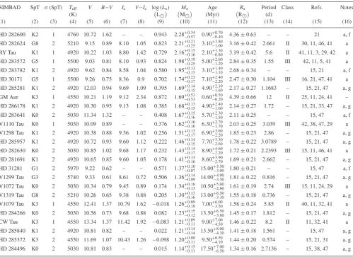
Figure 2. HR diagrams constructed from the Siess et al. (2000) PMS evolutionary models for the ONC sample (left) and Taurus–Auriga (right). The mass tracks (dashed black lines) are shown (from right to left) for 0.1, 0.2, 0.3, 0.4, 0.5, 0.6, 0.8, 1.0, 1.2, 1.5, 2.0, 2.5, and 3.0 Mstars. Isochrones (black dotted lines) are shown (from upper right to lower left) for ages 0.01, 0.05, 0.2, 0.5, 2, 5, 10, and 60 Myr. The position of the ZAMS is shown as a solid black line for 0.7–3.0Mstars. The solid red line marks the age at which each mass of star develops a radiative core according to equation (6). Stars that fell to the left of this line were removed from further analysis. An average error bar is included for reference in the lower left of each plot.
3.3 Stellar masses and ages
Stellar masses and ages were calculated fromTeff and L using
Siess et al. (2000) PMS model isochrone fitting. The models are applicable to stars above 0.1 Mand we apply an upper mass limit of 3.0 Mas stars more massive than this are not T Tauri stars. The range of stellar ages covered by the models extends from the stellar birth line to the ZAMS but a star older than∼10 Myr is unlikely to be a member of the ONC or Taurus–Auriga (see Section 3.4.1). The corresponding HR diagrams for our ONC and Taurus–Auriga samples are shown in Fig.2. Stars that lay outside of the imposed boundaries could not be assigned a stellar mass or age.
We use the Siess et al. (2000) PMS evolutionary models to trans-late the errors inLandTeff(in terms of the error in spectral type)
into estimates of errors on stellar mass and age. We do not consider errors within the PMS evolutionary models themselves; a discus-sion of these can be found in Siess (2001). The errors on log (Teff)
and log(L/L) define the major and minor axes of an ellipse in the HR diagram. The corresponding ellipse inM– Age space was calculated by iteratively tracing around the outside of the ellipse in log (Teff) – log (L/L) space and calculating the stellar mass and
age at each point. The maximum and minimum values of stellar mass and age calculated via this process were then used to estimate errors on the stellar mass and age for each star.
This method results in upper and lower bounded errors that are not symmetric with the difference being most apparent for the errors on the age estimates. Contraction occurs on a Kelvin–Helmholtz time-scale,tKH∝1/R, such that the rate of contraction slows with
time. This causes the isochrones to ‘bunch up’ in the HR diagram at older ages, producing upper bounded age errors that exceed the lower bounded errors.
Where the errors in log (Teff) – log (L/L) space exceeded the
bounds imposed by the Siess et al. (2000) model limits, the upper and lower bounds to stellar masses and ages were assigned individ-ually after conservative, by-eye inspection of the HR diagram.
3.4 Stellar radii
Under the assumption that the spread inL observed in our ONC and Taurus–Auriga samples is indicative of a real spread in stellar radii, we calculateRdirectly fromTeffandLusing
R
R =
L
L 1/2T
eff,
Teff,
2
, (12)
whereTeff, =5771.8 K (Mamajek2012).
It has been suggested that the observed spread inLis a conse-quence of a combination of observational and astrophysical uncer-tainties such as contamination by unresolved binaries, photometric variability, and inadequate correction for variable extinction (Hart-mann2001) rather than of a true spread inR. Although these effects all contribute to the differences inLthroughout the regions con-sidered, they have been found not to explain the full scale of the observed spreads (Burningham et al.2005; Preibisch & Feigelson 2005; Hillenbrand, Bauermeister & White2008; Slesnick, Hillen-brand & Carpenter2008; Da Rio et al.2010; Preibisch2012). In addition, Jeffries (2007) estimatedRindependently ofLandTeff
by combining projected stellar rotational velocities and rotational periods for stars in the ONC. Even after accounting for observa-tional uncertainties and random inclinations of the stellar rotation axes, the spread inRwas still observed.
3.4.1 Luminosity spreads as indicators of true age spreads
Our use ofTeffandLto derive individual ages for the stars in our
sample (Section 3.3) further assumes that the observed spread in
L(which we have attributed to a real spread inR) corresponds to a real spread in age. The question of whether this assumption is correct has been heavily debated in the literature (see e.g. Jeffries 2012; Soderblom et al.2014for recent reviews).
Certain studies have argued that the observed spread inR is produced by magnetic effects reducing convective efficiency or
at University of St Andrews on December 8, 2014
http://mnras.oxfordjournals.org/
significant spot coverage on the stellar surface (e.g. Spruit & Weiss 1986; Jackson & Jeffries2014). However, Chabrier, Gallardo & Baraffe (2007), Morales et al. (2010), and Feiden & Chaboyer (2014) find that the level of radius inflation produced by the inhibi-tion of convective efficiency is negligible (∼0.1–2 per cent) for fully convective stars. In addition, by considering observed spot temper-atures of K and early-M stars at 82–90 per cent of photospheric temperature (Boyajian et al.2012) and observed spot coverage of a few per cent to∼40 per cent (O’Neal, Neff & Saar1998; Barnes & Collier Cameron2001; Barnes, James & Collier Cameron2004; O’Neal et al.2004; Morin et al.2008; Hackman et al.2012), Feiden & Chaboyer (2014) found that starspots could only produce the degree of radial inflation inferred fromLspreads if unattainably high interior magnetic field strengths were present.
Alternatively, episodic accretion during the assembly phase with mass accretion rates≥10−5M
yr−1has been proposed as a method
of producing the observed spread in stellar radii (Tout, Livio & Bon-nell1999; Baraffe et al.2002; Baraffe, Chabrier & Gallardo2009). Depending on the amount of accretion kinetic energy absorbed by the star during this phase, the star can either contract at a greater rate and then remain at almost constant radius for∼10 Myr or it can inflate to larger radii before quickly contracting back to the non-accreting isochrone expected of its mass and age (Baraffe et al. 2009; Littlefair et al.2011). Thus, the stellar radius would be more an indication of accretion history rather than age. However, the abil-ity of this mechanism to produce the observed L spreads at low masses has been contested (Hosokawa, Offner & Krumholz2011) and depends on the initial protostellar mass assumed in the ‘cold accretion’ models (Baraffe, Vorobyov & Chabrier2012).
Using alternative age diagnostics such as lithium depletion levels has revealed that a few per cent of ONC and Taurus–Auriga PMS members are consistent with being≥10 Myr old (Palla et al.2007; Sacco et al.2007). Furthermore, Sergison et al. (2013) determined the ages of stars within the ONC and NGC 2264 using lithium de-pletion and PMS isochrones, finding a modest correlation between the two age indicators. With this in mind, we assume that the age spreads in the ONC and Taurus–Auriga are real and we use the individual isochronal ages to study the evolution ofj.
3.5 Rotation periods
The periodic nature of PMS stars has been used to determine stellar rotation periods using both optical and infrared (IR) wavelengths. For both Class II and Class III PMS stars, this observed periodicity can be attributed to cool starspots on the stellar surface. These reduce the flux received from the star at a rate determined by its rotational period (Carpenter et al.2001; DeWarf et al.2003; Grankin et al.2008; Frasca et al.2009). Additionally, for Class II PMS stars, magnetospheric accretion of disc material can produce hotspots on the stellar surface. These hotspots lead to an increase in flux received from the star, modulated by rotation in the same way as for the cool starspots.
Periodic flux changes in the near-IR (NIR) and mid-IR (MIR) can also be caused by temperate, opacity, or geometric changes in the inner disc (Bouvier et al.2003; Alencar et al.2010; Morales-Calder´on et al.2011; Artemenko, Grankin & Petrov2012; Cody et al. 2014). When these changes arise from regions in the disc close to the corotation radius, they can be used as indicators of stellar surface rotation rates.
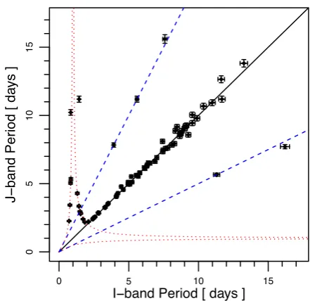
[image:8.595.314.535.53.267.2]Problems with the measurement of stellar rotation periods arise if multiple sources of periodicity are present. In such a case, the measured rotation period may only be a fraction of its actual value.
Figure 3. Example of the analysis undertaken to check for the effects of beats (red dotted lines) and harmonics (blue dashed lines) in the ONC sample. TheI-band periods are from Herbst et al. (2002), Parihar et al. (2009) and Rodr´ıguez-Ledesma, Mundt & Eisl¨offel (2009) and theJ-band periods are from Carpenter, Hillenbrand & Skrutskie (2001). Stars located on the solid black line have the same measured rotation period in both the optical and NIR.
Additionally, if observations are taken at a single longitude, the Earth’s day–night cycle imposes a 1 d sampling interval such that rotation periods of∼1 d can have a beat period,B, recorded rather than the true rotational period,P(Cieza & Baliber2006), where
1
B = ±1 d−
1± 1
P. (13)
We gathered previously published rotation periods from the liter-ature as detailed in Tables1and2for the ONC and Taurus–Auriga samples, respectively. Where errors for the rotation period were not reported, a conservative estimate of 0.01 d was assumed. In the cases, where multiple rotation periods were available for the same star, we checked for the effects of harmonics and beats, described above. An example of this analysis is shown in Fig.3for stars in the ONC. Any rotation periods that appeared to show evidence of these phenomena were removed from Tables1and2.
All rotation periods for members of Taurus–Auriga were mea-sured at optical wavebands whereas those for members of the ONC were measured at optical, NIR, or MIR wavebands. A general agree-ment between rotation periods measured at optical and NIR wave-lengths was found, as shown in Fig.3. The major differences be-tween the optical and IR rotation periods can be explained in terms of either harmonics or beats phenomena. We flagged all rotation periods longer than 15 d and removed them from further analysis. It is unlikely that these trace photospheric rotation and are more likely to be caused by occultation of the stellar surface by disc material ex-terior to the corotation radius (Artemenko, Grankin & Petrov2010; Cody et al.2014).
3.5.1 Central densities and the radius of gyration
Once the ages and stellar masses had been calculated and the fully convective limit imposed (see Section 3.3), we linearly interpolated the individual central densities from Siess et al. (2000) PMS core
at University of St Andrews on December 8, 2014
http://mnras.oxfordjournals.org/
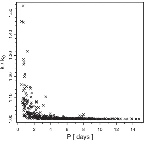
Figure 4. The relationship between stellar rotation period,P, and the radius of gyration,k, normalized to that of a perfect sphere,k0=(2/3)1/2for the
fully convective stars in the ONC and Taurus–Auriga withP<15 d. For all but a few of the fastest rotators, the stars in our sample are well approximated by perfect spheres.
isochrones. Combining these with the stellar rotation periods al-lowed us to calculate the radius of gyration,k, for each individual source using equation (4). Fig.4shows the relationship between the radius of gyration and the rotation period for the fully convec-tive stars in our combined ONC and Taurus–Auriga sample with
P<15 d. For all but a few of the fastest rotators, the stars are well approximated by perfect spheres.
As a final check of the rotation periods, we ensured that none of the rapidly rotating stars in Fig.4appeared to be rotating at rates exceeding break-up velocity. An object of mass,M, rotation period,
P, and equatorial radius,Req, will break apart if the acceleration due
to the centripetal force,
acent=
4π2R eq
P2 , (14)
exceeds the acceleration due to gravity,
agrav=
GM
R2 eq
. (15)
For the more rapidly rotating stars, the stellar shape will differ from a perfect sphere with the star becoming more distended around its equatorial regions. Following Chandrasekhar (1935),
Req
R,0
=a−bP2(θ=0), (16)
whereaandbare given by equations (3) and (4),R,0is the radius
of a non-rotating star,θis the usual polar angle, andP2(θ =0) is
the second order Legendre polynomial. This enables us to define a critical rotation period,
Pcrit=
2πR3/2 eq
(GM)1/2, (17)
such that ifP<Pcrit, the object will break apart.
We can use the critical rotation period to define a critical specific stellar AM,jcrit, using equation (1). We remove any stars from our
sample for which
j
jcrit
= 2πR
3/2 eq
(GM)1/2P >1. (18)
We found that 10 of the fully convective stars in our ONC sample havej ≥jcrit. All of these stars are at the low mass end of our
sample, with spectral types of M3.5 to M5.5. 9 of the 10 fully convective stars for whichj≥jcrithave only one recorded rotation
period, each measured at a fraction of 1 d. It is possible that these rotation periods are affected by the beat phenomena. For the other fully convective star, the rotation period is measured at 1.18 d but its luminosity is very high for its spectral type (M5). Thus, the stellar radius is much larger than other stars of a similar spectral type. It is possible that this luminosity is overestimated for this star, perhaps due to the presence of an unresolved binary (see Section 3.2.1).
3.5.2 Cluster membership: removing contamination from period distributions
The ONC is part of the much larger Orion A cloud and is surrounded by neighbouring regions of star formation (Hillenbrand1997; Alves & Bouy2012; Bouy et al.2014). In previous studies of ONC rotation period distributions, the inclusion of these regions has blurred the location of the peak of rapid rotators as well as the respective height of the two peaks, producing a unimodal distribution (e.g. Rebull 2001). For this reason, it was imperative to ensure that our ONC sample was as clean as possible. Members of the Orion flanking fields and other neighbouring regions such as NGC 1980, L1641N, L1641W, and NGC 1981 were removed from the sample. Only stars that lay within the ‘traditional’ region of the ONC (84.◦1≤RA≤
83◦.0 and−5.◦0≤Dec≤−5◦.7; Cieza & Baliber2007) were retained. Even with this cut applied to right ascension and declination, the ONC sample could be contaminated by members of the somewhat overlapping clusters L1641N and NGC 1980 (Alves & Bouy2012; Bouy et al.2014). All objects listed in Hillenbrand (1997) as having a membership probability <98 per cent were removed from the sample and any additional non-members were removed by cross-referencing with the recent studies of Fang et al. (2013) and Pillitteri et al. (2013).
3.5.3 Mass segregation
Due to the presence of a mass-rotation relation in PMS stars (Herbst et al.2000; Cieza & Baliber2007), we split our sample into two, mass-segregated groups. We do not base our mass cut directly on stellar mass due to the apparent age spread in our samples (Fig.2). Instead, we base our mass cut on spectral type with the ‘high mass’ sample having a spectral type of M2 or earlier and the ‘low mass’ stars being later than M2. This choice of spectral type cut off is based on the work of Cieza & Baliber (2007) who looked at the effect of varying the location of the spectral type cut on period dis-tributions in the ONC. They found that their results were consistent with a sudden change in stellar magnetic field strength or struc-ture between the M2 and M3 spectral types and that the bimodality of the ‘high mass’ sample was severely affected by even a small contamination by lower mass stars (Cieza & Baliber2007). At the range of ages included in our sample, this spectral type corresponds
at University of St Andrews on December 8, 2014
http://mnras.oxfordjournals.org/
to a stellar mass of∼0.35 M, the mass below which stars remain fully convective during their MS lifetimes (see Section 2).
3.6 Disc diagnostics
Observations of an accretion disc-rotation relation are dependent on the use of a reliable method to identify accretion discs. In the absence of circumstellar dust, the spectral energy distribution (SED) of a PMS star is purely photospheric in origin and resembles that of a blackbody (Lada & Wilking1984; Lada1987). During this phase, the PMS star is referred to as a Class III object. At earlier stages of formation, circumstellar dust is present around the star. This dust reprocesses incident stellar emission at longer wavelengths, giving rise to excess emission in the IR part of the SED. When this material fully envelopes the star, it is referred to as a Class I object. The rotation of the enveloping material around the central protostar means that high latitude regions of the envelope have lower AM than lower latitudes. Consequently, the infalling material flattens into a disc, allowing the stellar photosphere to become optically visible, and the star is identified as a Class II object (Adams, Lada & Shu1987).
For most of the stars in our Taurus–Auriga sample, the results of detailed SED modelling are available in the literature. We used these to identify the presence (or absence) of an IR excess and so define source as a Class II (or Class III) object (Kenyon & Hart-mann1995; Andrews & Williams2005; Luhman et al.2010; Rebull et al.2010). In addition, resolved (sub)millimetre observations have directly imaged discs around individual stars in Taurus–Auriga (Ki-tamura et al.2002; Rodmann et al.2006; Andrews & Williams2007; Guilloteau et al.2011). We used these identifications to supplement our Taurus–Auriga Class II sample.
For the ONC sample, the same detailed SED modelling was not available. Most early studies of PMS AM evolution in the ONC relied on NIR excesses and Hαequivalent widths (EW) to ascer-tain whether a PMS star hosted a circumstellar disc or was actively accreting, respectively. However, the magnitude of the IR excess at NIR wavelengths, and the HαEW, is dependent on stellar mass (White & Basri2003; Littlefair et al.2005; Cody et al.2014) and, due to the low contrast between photospheric and disc emission at NIR wavelengths, disc indicators relying onJ-,H-, orK-band emission were found to miss up to 30 per cent of discs detected at longer wavelengths (Hillenbrand et al.1998). In addition, obser-vations used to derive NIR excesses were often taken at different epochs and were consequently affected by the intrinsically periodic nature of PMS stars (Section 3.5). More recently,SpitzerIRAC have provided high-resolution, contemporaneous observations between 3.6 and 70μm which allow for more reliable PMS classification.
We gathered 2.2, 3.6, 4.5, 5.8, and 8.0μmSpitzerIRAC fluxes from Rebull et al. (2006), Cieza & Baliber (2007), Prisinzano et al. (2008), and Morales-Calder´on et al. (2011). Over this wavelength range, the spectral index,αi−(i+1), (Lada1987) is defined as
αi−(i+1)= −
logλi+1Fλi+1
−logλiFλi
log (λi+1)−log (λi) , (19)
where i = 1, 2, 3, 4 and refers to the waveband such that [2.2,3.6,4.5,5.8]μm are wavelengths [λ1,λ2,λ3,λ4].
We made sure that our Class II and Class III samples were not contaminated by more embedded objects. Any source that displayed an increasing SED over the 2.2–8.0μm wavelength range was re-moved from further analysis. We made no attempt to classify these objects as either Class 0 or Class I and these objects are included in Tables1and2amongst the unclassified sources.
To identify the Class II sources in our ONC sample, we followed methods employed in Hartmann et al. (2005) and Rebull et al. (2006). We selected all sources for which [3.6]−[8.0]>1.0, or 0.2<[3.6]−[4.5]<0.7 and 0.6<[5.8]−[8.0]<1.0. These are slightly more restrictive criteria than others employed usingSpitzer
IRAC colours (e.g. Megeath et al.2004) but should enable us to compile as pure a set of Class II objects as possible. Identification as Class II required agreement between the four studies from which we took theSpitzer IRAC fluxes. Where identifications did not agree, the source remained unclassified. It is hoped that this will reduce contamination from transitional discs and ‘flat’ spectrum objects.
The Class III objects were selected from the remaining unclas-sified sources. A Class III PMS star displays purely photospheric emission as it lacks the IR excess seen for disced objects. As such, to be identified as a Class III object, a star must satisfy [2.2]− [3.6]<0.5, [3.6]−[4.5]<0.2, [4.5]−[5.8]<0.2, and [5.8]− [8.0]<0.2 (Prisinzano et al.2008). Alternatively, objects were also identified as purely photospheric if they were detected atIcband
but not detected at wavelengths longer than 3.6μm. Again, just as with the Class II sample, agreement between the sources ofSpitzer
IRAC fluxes was required in order for the source to be identified as Class III.
4 R E S U LT S A N D D I S C U S S I O N
Tables1and2display the data gathered for all members of the ONC and Taurus–Auriga, respectively, that have not previously been identified as binary or multiple (Section 3.2.1) and for which a spectral type was available in the literature (see Section 3.5.2 for details on ONC membership). Rotation periods found to be affected by beats and harmonics (Section 3.5) are not included.
As outlined in Section 3.5, we applied several cuts to these data. All stars with (i) rotation periods longer than 15 d, (ii) isochronal ages greater than their individualtcore, or (iii) withj/jcrit>1 were
removed from the analysis (see Sections 3.3 and 3.5 for details), although they remain included in Tables1and2.
Using equation (1), we calculatedjfor all stars for which we had a measured rotation period, stellar radius and an estimate of its age. In total, we were able to calculatejfor 352 and 32 fully convective stars within the ONC and Taurus–Auriga, respectively. Of these, 226 ONC and 24 Taurus–Auriga stars were able to be classified as Class II or Class III. We imposed a cut to the data at a spectral type of M2 in order to study our low mass and high mass fully convective PMS stars separately. The final classified samples consisted of 91 ONC and 20 Taurus–Auriga stars of spectral types K0 to M2 together with a further 135 ONC and 4 Taurus–Auriga stars of spectral type later than M2. These formed our high mass and low mass samples, respectively.
Before considering howjevolves with age for the various sam-ples in Section 4.2, we first consider its expected time evolution based on theoretical considerations in Section 4.1.
4.1 Evolution of specific angular momentum during PMS contraction: theory
It is clear from equation (1) that, asj∝R2
/P, the specific AM
evolution of a PMS star depends on the stellar contraction and how the stellar rotation period evolves with time. We consider these quantities in turn. For a contracting fully convective polytropic PMS
at University of St Andrews on December 8, 2014
http://mnras.oxfordjournals.org/
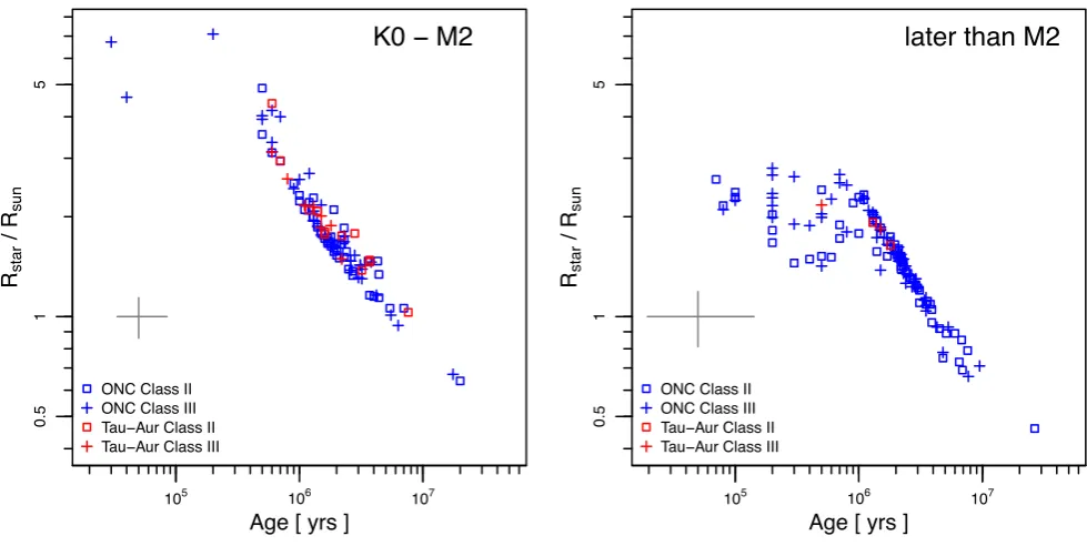
Figure 5. Evolution of the stellar radius of Class II (open squares) and Class III (crosses) stars in the ONC (blue) and Taurus–Auriga (red). The left- and right-hand panels show the contraction rates for the high and low mass samples, respectively. An average error bar is located in the bottom left of each plot for reference. We observe a consistent contraction rate in both Class II and Class III objects. Our fitted gradients are presented in Table3and are slightly steeper than, but in rough agreement with, those expected from purely theoretical considerations of contraction on a Hayashi track.
Table 3. Results of minimum-χ2fitting to equation (21) for (i) the ONC sample alone and (ii) the com-bined ONC and Taurus–Auriga samples. Column 1 lists the sample name; columns 2 and 3 list the value ofβ1for the high and low mass samples, respectively.
Sample Minimum-χ2β
1
High mass Low mass
(1) (2) (3)
ONC Class II 0.53±0.09 0.42±0.07 ONC Class III 0.53±0.08 0.56±0.14 ONC & Tau Class II 0.53±0.08 0.42±0.07 ONC & Tau Class III 0.53±0.07 0.56±0.14
star, descending a Hayashi track in the HR diagram (Teff≈const.),
it is straightforward to show that
R∝t−1/3 (20)
(e.g. Lamm et al.2005).
Fig. 5 shows the rate of stellar contraction in our ONC and Taurus–Auriga samples. We used the numerical recipeFITEXY
rou-tine inIDLto produce a minimum-χ2fit to the linear relation
log(R)= −β1log(t)+γ1. (21)
This routine can account for symmetric heteroscedastic errors in bothRand age. However, due to the method of their estimation, the errors in stellar age are not symmetric (Section 3.3). For each value of stellar age, we adopt the maximum of its lower and upper bounded error for the minimum-χ2fitting procedure. The results
of this analysis are presented in Table3. Under the assumption that the radius and age spreads that we observe in our ONC and Taurus–Auriga samples are real (see Section 3.4), we find that the rate of stellar contraction observed in our ONC and Taurus–Auriga
samples is steeper than, but in rough agreement with, that expected from equation (20). Taking β1 = 1/3 (equation 20), we would
expectjto evolve asj∝t−2/3P−1.
If, over a time-scale of a few Myr, the rotation period of a star varies, on average, as a simple power law of the form
P ∝tn, (22)
then
j∝t−2/3−n. (23)
There then exist three scenarios:n=0 corresponds to a star that is evolving at a constant rotation rate;n>0 to a star that is spinning up; andn<0 to a star that is spinning down. The evolution of the rotation period and, therefore, ofjwill differ for Class II and Class III stars with the former being driven by the astrophysics of the star– disc interaction. Assuming that, during the Class II phase, a star is locked to its disc – accreting and contracting without spinning up, with the surface rotation rate fixed to the Keplerian rotation rate at the disc truncation radius, a common assumption of PMS rotational evolution models (e.g. Gallet & Bouvier2013) – thenn=0. Thus, we would expectjto reduce with age asj∝t−2/3.
Class III stars, which have lost their accretion discs, would con-serve AM as they contract such thatj=const. (neglecting the likely small loss of AM in the stellar wind). Therefore, for Class III stars, we expectn= −2/3 such that they spin up asP∝t−2/3
as they continue their gravitational contraction. However, as we discuss in the following subsection, this is not what we observe. Instead, assuming the inferred luminosity spreads for the ONC and Taurus–Auriga are indicative of real age spreads (see Section 3.4.1), our results suggest thatj∝t−β2withβ
2≈2–2.5 for both Class II
and Class III sources.
at University of St Andrews on December 8, 2014
http://mnras.oxfordjournals.org/