Artificial neural network approaches and compressive sensing techniques for stochastic process estimation and simulation subject to incomplete data

(1)

Artificial Neural Network approaches and Compressive

Sensing techniques for stochastic process estimation and

simulation subject to incomplete data

Thesis submitted in accordance with the requirements of the University of Liverpool for the degree of Doctor in Philosophy

by Liam Anthony Comerford

(2)

(3)

Declaration

I hereby confirm that the results presented in this dissertation are from my own work, developed in conjunction with my supervisors, and that I have not presented anyone else’s work as my own and that full and appropriate acknowledgements have been given where references have been made to the work of others.

Liam Anthony Comerford

(4)

(5)

Acknowledgements

Great appreciation and gratitude for the help and support are extended to the following persons who have contributed in making this work possible.

Professor Michael Beer and Dr. Ioannis Kougioumtzogloufor their continued guidance throughout the project. They have both shown great patience and invested significant time and effort into facilitating my studies, for which I consider myself very fortunate.

Dr Edoardo Patelli and Dr. Matteo Broggi for helping to prepare my codes for cluster computing, and fixing numerous associated problems, despite having no di-rect investment in my work. The help was greatly appreciated.

Mr Adam Mannis for his general guidance and support. He knows all there is to know about writing reports and how to present them.

Mr Marco DeAngelis for always being around to bounce ideas off and acting as an efficient alternative to the Matlab help files when I needed a function quickly.

Dr. Ioannis Mitseas for his happy-go-lucky optimistic charm.

I would like to thank my Family for their support, even though they don’t really know what I’m up to; and also my friends, particularly John Connor and Matthew Kent for providing frequent ant-related distractions.

(6)

(7)

Abstract

This research is themed around development of tools for discrete analysis of stochastic processes subject to limited or missing data; more specifically, estimation of stochastic process power spectra from which new process time-histories may be simulated. In this context, the author proposes three novel approaches to power spectrum estimation subject to missing data which comprise the main body of this work. Of particular importance is the fact that all three approaches are adaptable for use in both stationary and evolutionary power spectrum estimation. Numerous arrangements of missing data are tested to simulate a range of possible scenarios to demonstrate the versatility of the proposed methodologies.

The first of the three approaches uses an artificial neural network (ANN) based model for stochastic process power spectrum estimation subject to limited / missing data. In this regard, an appropriately defined ANN is utilized to capture the stochastic pattern in the available data in an “average sense”. Next, the extrapolation capabili-ties of the ANN are exploited for generating realizations of the underlying stochastic process. Finally, power spectrum estimates are derived based on established frequency (e.g. Fourier analysis), or versatile joint time-frequency analysis techniques (e.g. har-monic wavelets) for the cases of stationary and non-stationary stochastic processes, respectively. One of the significant advantages of the approach relates to the fact that no a priori knowledge about the data is assumed.

The second approach uses compressive sensing (CS) to solve the same problem. In this setting, further assumptions are imposed on the nature of the underlying process of interest than in the ANN case, in particular that of sparsity in the frequency do-main. The advantages being that when compared to ANN, significant improvements in efficiency and accuracy are achieved with increased reliability for larger amounts of missing data. Specifically, first an appropriate basis is selected for expanding the signal recorded in the time domain. As with the ANN approach, Fourier and harmonic wavelet bases are utilized. Next, an L1 norm minimization procedure is performed for obtaining the sparsest representation of the signal in the selected basis. Further, an adaptive basis procedure is introduced that significantly improves results when working with stochastic process record ensembles.

(8)

(9)

List of Figures

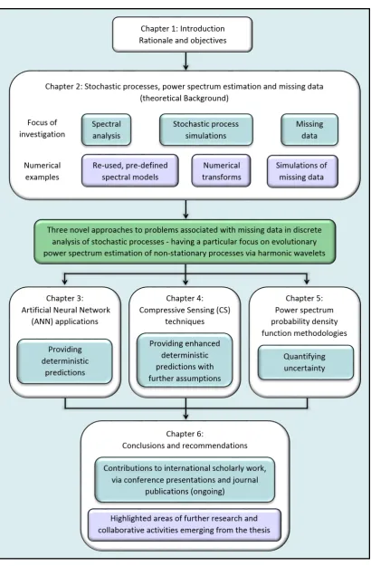
1.1 Thesis structure . . . 4

2.1 Example sample space with two events mapped to the real line . . . 5

2.2 Three sample functions of a stochastic process . . . 9

2.3 Example of aliasing . . . 13

2.4 A measured sinusoid (top) and the DFT assumption (bottom) . . . 14

2.5 Spectral leakage around 5 rad/s in the frequency domain taken from the DFT of the signal in Figure 2.4 . . . 14

2.6 Cosine signal and its absolute Fourier coefficients . . . 15

2.7 Cosine signal (lasting for half the sample) and its absolute Fourier coef-ficients . . . 16

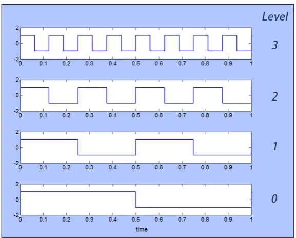
2.8 Levels 0 to 3 of the Haar wavelet . . . 18

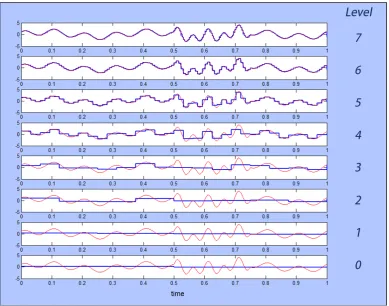
2.9 Levels 0 to 7 of a Haar wavelet decomposition of Eq.2.39 . . . 19

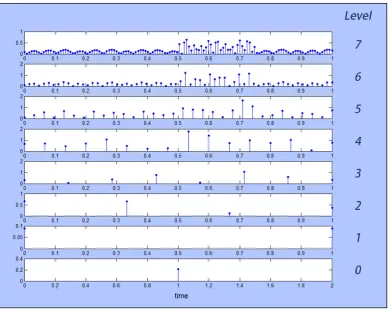
2.10 Levels 0 to 7 of Haar wavelet coefficients representing a signal . . . 20

2.11 Daubechies wavelets in the frequency domain constructed from 4, 6, 10 and 20 coefficients . . . 21

2.12 Dyadic harmonic wavelets in the frequency domain starting from Level -1 22 2.13 Harmonic wavelets in the frequency domain with n−m= 8Hz . . . 23

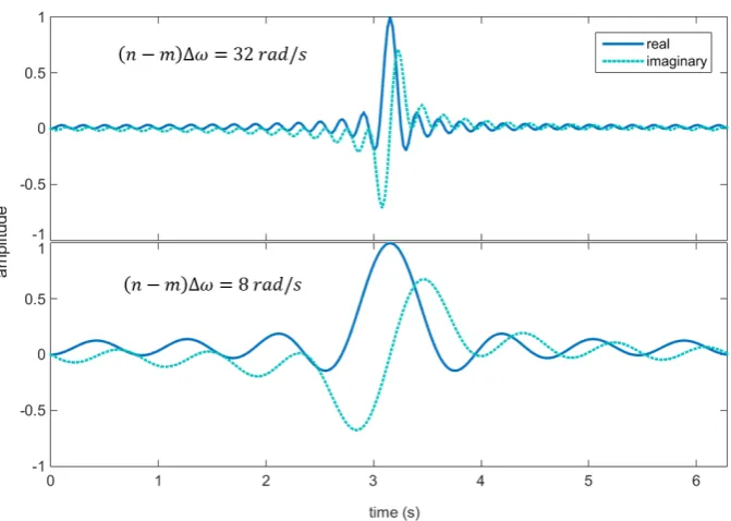
2.14 Comparison of Harmonic wavelets in the time domain for high (top) and low (bottom) resolution in time . . . 23

2.15 FFT algorithm for producing harmonic wavelet coefficients . . . 25

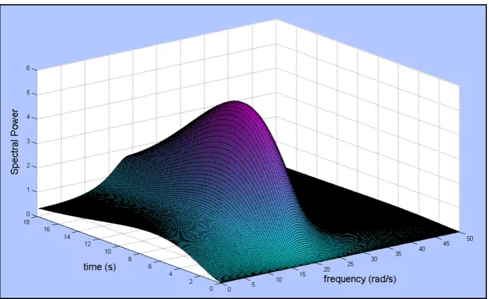
2.16 Example non-stationary power spectrum process model . . . 29

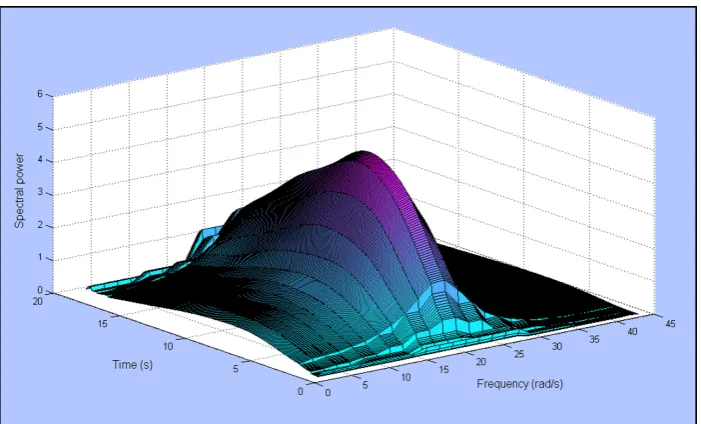
2.17 Reconstruction of Figure 2.16 via GHWT from 500 realizations . . . 30

2.18 Depiction of reverse signal padding . . . 30

2.19 Reconstruction of Figure 2.16 via GHWT from 500 realizations with reverse signal padding . . . 31

2.20 Reconstruction of Figure 2.16 via GHWT from 500 realizations with decreasing frequency resolution near the edgest= 0s&t= 18s . . . 32

2.21 Example stochastic process spectrum from Eq.2.65 with a = 0.5, ζ = 0.35 andωg= 15 . . . 32

2.22 Example JONSWAP spectrum from Eq.2.66 with α = 0.03, ωp = 0.7, γ = 3.3,σ = 0.07 for (ω≤ωp), andσ= 0.09 for (ω > ωp) . . . 33

2.23 Example Clough-Penzien spectrum from Eq.2.67 withS0= 0.07,ωf = 1, ζf = 0.6,ωg = 10 and ζg = 0.4 . . . 34

2.24 Example envelope function from Eq.2.68 with k= 4,a= 0.3 and b= 0.6 34 2.25 Example time-modulated stochastic process model based on Eq.2.65 . . 34

2.26 Example non-stationary, non-separable spectrum from Eq.2.69 . . . 35

2.27 Complete regularly sampled time-series (top) compared to the same sig-nal with missing data (bottom) . . . 36

(12)

3.1 Model of ANN neuron with synaptic weights . . . 42

3.2 Example feed-forward ANN architecture (4-2-2) . . . 43

3.3 A single neuron (or perceptron) in an ANN . . . 43

3.4 ANN input selection for training . . . 46

3.5 ANN process prediction procedure . . . 47

3.6 Procedure for filling missing data during training on a stationary process 48 3.7 Examples of usable training sets when training with missing data . . . . 48

3.8 Error convergence of ANN trained on samples with and without missing data . . . 49

3.9 ANN trained on data with large gap, then used to fill the gap to give a complete time-history . . . 49

3.10 Procedure for filling missing data during training on a non-stationary process . . . 50

3.11 Flowchart depicting step-by-step ANN approach to process learning sub-ject to missing data . . . 51

3.12 Target and estimated spectrums for 25 averaged samples using FFT directly with zeros and FFT of ANN predictions - 30% missing data at random locations . . . 53

3.13 Target and estimated spectrums for 25 averaged samples using FFT directly with zeros and FFT of ANN predictions - 50% missing data at random locations . . . 53

3.14 Non-stationary target spectrum . . . 55

3.15 GHWT estimated spectrum with no missing data using 25 averaged time-histories . . . 55

3.16 GHWT estimated spectrum with 50% missing data at random locations for 25 averaged time-histories using ANN . . . 56

3.17 GHWT spectrum with 50% missing data at random locations for 25 averaged time-histories using zero-filled gaps . . . 57

3.18 GHWT estimated spectrum with 50% missing data at random locations for 25 averaged time-histories using linear interpolation . . . 57

3.19 GHWT estimated spectrum with 50% missing data at two fixed-interval locations for 25 averaged time-histories using ANN . . . 58

3.20 GHWT estimated spectrum with 50% missing data at two fixed-interval locations for 25 averaged time-histories using zero-filled gaps . . . 58

3.21 Non-separable evolutionary power spectrum . . . 59

3.22 GHWT estimated non-separable spectrum with no missing data for 25 averaged time-histories . . . 59

3.23 GHWT non-separable spectrum with 50% missing data at random loca-tions for 25 averaged time-histories using ANN . . . 60

3.24 GHWT non-separable spectrum with 50% missing data at random loca-tions for 25 averaged time-histories using zero-filled gaps . . . 60

3.25 Average difference between estimated non-separable power spectrum from 100 time histories compatible with Eq.2.69 and ANN and zero padded reconstructions. Samples suffer from 50% missing data in uniformly dis-tributed random locations. . . 61

4.1 Graphical output of Eq.4.10 with randomly selected points to sample . . 66

4.2 Randomly sampled points without original signal . . . 66

4.3 Eq.4.10 represented in the frequency domain as a sparse signal with CS estimation of frequency domain coefficients from Figure 4.1 . . . 66

(13)

4.5 Minimum L2 and L1 solutions to the equation,a+ 2b= 1 . . . 68 4.6 Minimum L1 solution to the equation, a+ 2b = 1 with tolerance, e for

noise vector, z. . . 69 4.7 (a) Full windspeed record. (b) Full record with missing data. (c,d)

Records with 50% missing data in random locations, down-sampled and reconstructed via L1 and L2 minimization of harmonic wavelets respec-tively. Data provided by [74] . . . 70 4.8 Signal acquisition of Eq.4.19 at every point in N note thatxf is sparse

in the Fourier matrixAf, henceyhas only two entries (one representing

cos(6t) and one representing cos(12t)) . . . 71 4.9 Signal acquisition of Eq.4.19 at N₂ uniformly distributed random

loca-tions overxf for CS with a Fourier basis . . . 72

4.10 Eq.4.19 with N₂ uniformly distributed missing data over xf set in CS

framework with a Fourier basis . . . 73 4.11 Fourier sampling matrix construction with missing data . . . 74 4.12 Non-redundant orthogonal Harmonic wavelet basis construction using

IFFT and nested for-loops . . . 74 4.13 Harmonic wavelet sampling matrix construction with missing data . . . 75 4.14 Least squares minimization solution of Eq.4.21 . . . 77 4.15 L1 minimization solution of Eq.4.21 . . . 78 4.16 L1 minimization solution of Eq.4.21 after applying the re-weighting

ma-trix in Eq.4.22 . . . 78 4.17 Example of basis re-weighting procedure promoting sparsity using only

average basis coefficients to update the weights (noticey1 throughy3 do not change as they were originally estimated in aand c) . . . 79 4.18 CS with adaptive basis method using a Fourier basis) . . . 82 4.19 Example JONSWAP process (top) and the same process with 65%

miss-ing data (bottom) . . . 83 4.20 JONSWAP power spectrum reconstruction from 10 stationary process

records via L1 minimization and scaled, zero-padding for 65% missing data at uniform random locations . . . 84 4.21 JONSWAP power spectrum reconstruction from 10 stationary process

records via L1 minimization and scaled, zero-padding for 50% missing data over randomly located fixed intervals of lengthN0/32 . . . 84 4.22 Eq.2.65 power spectrum reconstruction from 10 stationary process records

via L1 minimization and scaled, zero-padding for 50% missing data at uniform random locations . . . 84 4.23 Separable target spectrum drawn from Eq.4.23 . . . 85 4.24 Averaged GHWT spectrum estimation with no missing data using 25

time-histories compatible with Eq.4.23 . . . 86 4.25 Non-separable target spectrum drawn from Eq.2.69 . . . 86 4.26 Averaged GHWT spectrum estimation with no missing data using 25

time-histories compatible with Eq.2.69 . . . 86 4.27 Separable earthquake power spectrum reconstruction from 25

station-ary process records via zero-padding for 50%/ missing data at uniform random locations . . . 87 4.28 Separable earthquake power spectrum reconstruction from 25 stationary

(14)

4.29 Separable earthquake power spectrum reconstruction from 25 stationary process records via zero-padding for 50% missing data over randomly located fixed intervals . . . 88 4.30 Separable earthquake power spectrum reconstruction from 25 stationary

process records via L1 minimization for 50% missing data over randomly located fixed intervals . . . 89 4.31 Non-separable earthquake power spectrum reconstruction from 25

sta-tionary process records via zero-padding for 50% missing data at uniform random locations . . . 89 4.32 Non-separable earthquake power spectrum reconstruction from 25

sta-tionary process records via L1 minimization for 50% missing data at uniform random locations . . . 89 4.33 Non-separable earthquake power spectrum reconstruction from 25

sta-tionary process records via zero-padding for 50% missing data over ran-domly located fixed intervals . . . 90 4.34 Non-separable earthquake power spectrum reconstruction from 25

sta-tionary process records via L1 minimization for 50% missing data over randomly located fixed intervals . . . 90 4.35 (From top to bottom) single realization of Eq.2.69, single realization

from Figure 4.34 and a single realization of Figure 4.33 . . . 91 4.36 Comparison of stationary spectrum reconstructions . . . 92 4.37 Convergence of stationary spectrum reconstructions to a single estimate 92 4.38 Convergence of % error between estimated spectrum and target spectrum 92 4.39 a. Target spectrum for Eq.4.24 with no missing data, b, c & d. Spectrum

reconstructions with 75% missing data at random locations for CS with adaptive basis, CS without adaptive basis and zero-padding respectively 94 4.40 a. Target spectrum for Eq.4.24 with no missing data, b, c & d. Spectrum

reconstructions with 75% missing data over random intervals for CS with adaptive basis, CS without adaptive basis and zero-padding respectively 95 4.41 Average difference between estimated non-separable power spectrum from

100 time histories compatible with Eq.2.69 and adaptive basis CS and zero padded reconstructions. Samples suffer from 50% missing data in uniformly distributed random locations. . . 96 5.1 Continuous harmonic wavelet defined by Eq.2.44 with for k= 0, m= 1

and n= 6 . . . 102 5.2 Discrete harmonic wavelet defined by Eq.5.20 fork= 0,m= 1 and n= 6 103 5.3 Power spectral probability densities with 10% missing data replaced by

independent, identically distributed normal random variables . . . 105 5.4 Selected PDFs from Figure 5.3 at 6 rad/s, 12 rad/s and 24 rad/s. The

vertical lines show the estimated spectral power with no missing data for each PDF . . . 105 5.5 Power spectral probability densities with 20% missing data replaced by

independent, identically distributed normal random variables . . . 105 5.6 Selected PDFs from Figure 5.5 at 6 rad/s, 12 rad/s and 24 rad/s. The

vertical lines show the estimated spectral power with no missing data for each PDF . . . 106 5.7 Comparison of Monte-Carlo simulated PDF and numerical integration

solution for 105, 106 and 107 samples for 18 rad/s with 10% missing data 106 5.8 Non-separable earthquake power spectrum defined by Eq.2.69 . . . 107 5.9 Harmonic wavelet power spectrum for single time history compatible

(15)

5.10 PDFs of power spectral density for the single realization of Eq.2.69 shown in Figure 5.9 with 10% missing data in uniformly distributed random locations . . . 108 5.11 PDFs of power spectral density for the single realization of Eq.2.69 shown

in Figure 5.9 with 20% missing data in uniformly distributed random locations . . . 109 5.12 PDFs of power spectral density for a single realization of Eq.2.69 shown

in Figure 5.9 with 10% missing data near the beginning of the record . . 109 5.13 Additional explanation for interpreting Figures 5.10, 5.11 and 5.12 . . . 110 5.14 Selected PDFs from Figure 5.12 for k = 1 at 6 rad/s, 12 rad/s and 24

rad/s. The vertical lines show the estimated spectral power with no missing data for each PDF . . . 110 5.15 Selected PDFs from Figure 5.12 for k = 4 at 6 rad/s, 12 rad/s and 24

(16)

(17)

List of publications

A list of publications by the author that were produced as a result of the work docu-mented in this thesis are given here.

Conference proceedings

Comerford, L.A; Kusanovic, D.; Kougioumtzoglou, I.A.; Jensen, H.A.; Beer, M., “Struc-tural system response and reliability analysis subject to incomplete earthquake records”

Proceedings of the 12th International Conference on Applications of Statistics and Prob-ability in Civil Engineering (ICASP). (July 2015)

Comerford, L.A.; Kougioumtzoglou, I.A.; Beer, M., “Compressive sensing based power spectrum estimation from incomplete records by utilizing an adaptive basis” Proceed-ings of the IEEE Symposium Series on Computational Intelligence (SSCI), 2014 IEEE Symposium on Computational Intelligence for Engineering Solutions (CIES). (Decem-ber 2014)

Comerford, L.A.; Kougioumtzoglou, I.A.; Beer, M., “Uncertainty quantification in power spectrum estimation of stochastic processes subject to missing data”Proceedings of the 2nd International Conference on Vulnerability, Risk Analysis and Management.

(July 2014)

Comerford, L.A.; Kougioumtzoglou, I.A.; Beer, M., “A compressive sensing based ap-proach for estimating stochastic process power spectra subject to missing data Spec uncertainty”Proceedings of the 9th International Conference on Structural Dynamics (EURODYN), Reliability and robustness of dynamic systems. (July 2014)

Comerford, L.A.; Kougioumtzoglou, I.A.; Beer, M., “A compressive sensing based ap-proach for evolutionary power spectrum estimation subject to missing data”Proceedings of the 7th International Conference on Stochastic Mechanics (CSM).(June 2014) Comerford, L.A.; Kougioumtzoglou, I.A.; Beer, M., “An artificial neural network based approach for power spectrum estimation subject to limited and/or missing data” Pro-ceedings of the 11th International Conference on Structural Safety & Reliability (ICOS-SAR), Safety, Reliability, Risk and Life-Cycle Performance of Structures and Infras-tructures, pages 1083–1090, ISBN: 978-1-138-00086-5. (June 2013)

(18)

Journal articles

Comerford, L.A.; Kougioumtzoglou, I.A.; Beer, M., “A compressive sensing based ap-proach for evolutionary power spectrum estimation subject to missing data” - Proba-bilistic Engineering Mechanics. (Under review, submitted June 2015)

Comerford, L.A.; Kougioumtzoglou, I.A.; Beer, M., “Uncertainty quantification in power spectrum estimation of stochastic processes subject to missing data” – Inter-national Journal of Sustainable Materials and Structural Systems (IJSMSS). (Under review, submitted June 2015)

Comerford, L.A.; Kougioumtzoglou, I.A.; Beer, M., “An artificial neural network ap-proach for stochastic process power spectrum estimation subject to missing data” Struc-tural Safety 2014: Special issue on Engineering Analysis with Vague and Imprecise Information. Volume 52, Part B, Pages 150-160, ISSN 0167-4730. (January 2015)

Pedagogical work

(19)

Chapter 1

Introduction

1.1 Rationale and objectives

Probabilistic engineering simulations often require models for the engineering system excitation/response processes. For stochastic process model based Monte Carlo simula-tions to be reliable, modelling/estimation techniques often require a significant amount of data and/or some prior knowledge of the underlying physics of the process; i.e. the more data on which a model is built, the more statistically accurate the simulation is likely to be. The data collected is of course dependant upon the process that needs to be modelled. For system excitation (particularly civil engineering structures) we are often interested in environmental stochastic processes. To model an earthquake process, accelerogram data may be collected (ground acceleration set against time); to model the effects of wind, it may be important to capture changes in pressure against time; to model ocean storms and tidal patterns, the source data will likely take the form of water height over time. All of these examples have a common factor in that they are time-dependant. Although variation in the time-domain is not a requirement of stochastic processes in general, nor does it define a restriction for the methodologies presented herein, it provides a good basis for presenting many practical problems of a similar nature and in considering analysis of frequency dependant properties. In this regard, it is important to note that a time-based model definition of a stochastic process can take many forms. It could be as simple as an estimation of the mean and variance of a process, or as complex as a complete probability density function (PDF) with cor-relation defined for all time. Often, especially when dealing with processes that exhibit some underlying harmonic behaviour, an estimation of the process power spectral den-sity is key [1]. A reliable spectral model providing frequency dependant information can be of significant importance in investigating the response of an engineering system to stochastic input. However, a basic spectral model may only describe a stationary process, i.e. one in which the spectral content does not change over time. This as-sumption of stationarity often produces a poor approximation of the true process, as many important processes of interest are non-stationary in nature. For example, the frequency content of an earthquake induced excitation can change dramatically over its duration, and wind systems may contain short infrequent bursts that do not conform to the otherwise stationarity of the rest of the process. Hence, in many cases, realiza-tion of time-dependant properties of stochastic processes are also considered central to defining reliable spectral models [2, 3]. For these reasons, power spectrum estimation, and in particular its non-stationary form (in time) is a primary focus in this work.

(20)

all relevant features of the process. Practical reasons for having limited data include the following:

• Equipment failure

This is a possibility whenever using sensory equipment to detect and record stochastic processes. If a sensor becomes damaged, perhaps even as a result of the process itself, data may be lost.

• Sensor limitations

Sensors for detecting vibrations, displacements, pressures etc will operate to some threshold limits. High fidelity sensors with a wide operational range can be expensive, and so in some cases the equipment used to record a process may not be able to capture extreme features.

• Maintenance

Sensory equipment may not be designed to operate indefinitely and as a result, for long process recordings, may require intermittent maintenance.

• Bandwidth limitation

If sensors are used remotely then data must be transmitted wirelessly. The band-width required to receive uncompressed data from multiple sensors may be too great to process simultaneously. In these situations sensor data may be received selectively in bursts, producing gaps in what would otherwise be a constant data stream.

• Usage restrictions

It may be the case that to capture relevant data on the process of interest, expen-sive specialist equipment is required; equipment that may need to be rented or shared. Data that could have otherwise been captured, may have to be forfeited when a third party needs access to the equipment.

• Acquisition restrictions

It could be the case that there are practical difficulties in being able to set up equipment so that the process can be captured. For example, when using an earth based telescope to detect objects in outer space, both cloud cover and the earth’s rotation could prevent relevant data capture.

• Data corruption

When dealing with digital data, corruption is always a possibility; perhaps as a result of accidental electrical damage or even malicious attack.

(21)

from falsely detected peaks, spectral leakage and significant loss of power as the number of missing data increases. Other alternative approaches for spectral estimation in the case of non-uniform sampling may impose restrictions on the nature of the missing data; e.g., infrequent loss [10, 11] or assume that the underlying process comprises of a highly limited number of significant harmonic components [12, 13]. Additional challenges arise when dealing with non-stationary data. In this regard, to estimate the power spectrum of a non-stationary process, the Gabor transform [14], wavelets [15, 16, 17, 18, 19], chirplets [20] and the Wigner-Ville distribution [21, 22] present means of analysing the non-stationary spectral content of a signal. Nevertheless, many of the approaches for addressing missing data in the stationary case cannot be applied, at least in a straightforward manner for non-stationary cases, or assume that the process is locally stationary [23].

The limited breadth of tools available for spectral analysis of stochastic processes in cases of missing data has led the author to develop new approaches to these prob-lems, and is the primary motivating factor for this work. The need for such research is strongly supported by academic literature, and its applications are numerous in address-ing aspects of risk and uncertainty across multiple areas of engineeraddress-ing. In this thesis, three novel approaches to problems associated with spectral estimation under missing data are presented. Two of these centre around reconstructing incomplete/gappy data sets, providing full, uniformly sampled time-histories for further analysis. The third is a fundamentally different approach that aims to quantify the uncertainty in spectral estimates due to missing data probabilistically.

1.2 Organization of thesis

(22)

[image:22.595.71.482.97.723.2]

(23)

Chapter 2

Stochastic processes, power spectrum

estimation and missing data - an overview

2.1 Introduction

There is a wealth of information available on the subjects of stationary and non-stationary stochastic process spectral analysis, and how to mitigate problems caused by missing data, each method having its own advantages and disadvantages. As such, this section provides a brief review of relevant elements of stochastic process theory and spectrum estimation, as well as the motivations behind such analysis. This is followed by a definition of the problems associated with missing data in power spectrum estima-tion, along with the limitations of current spectral reconstruction methods. However, first, building blocks for stationary and non-stationary stochastic process representation applied in this doctoral investigation are discussed for completeness (this is primarily a review of probability theory, Fourier and Wavelet analysis).

2.2 Random variables & Stochastic processes

Probability concepts surrounding random variables and stochastic processes will be introduced here, providing a basis for signal transforms introduced in the next section.

2.2.1 Probability density functions

A random variable is a mathematical mapping from events on a probability space to the real line. It allows events to be represented in analytical form. If a real number,

x=X(ζ) is assigned to each possible outcome,X(ζ), of the probability space,S, then

X is defined on the real line and X = a, X ≤ a and a ≤ X ≤ b may be classed as events. An example is given in Figure 2.1 where events E1 and E2 may be defined by limits on the real line. Random variables may be discrete or continuous. Note that most continuous events are already in numerical terms and the mapping from the event space to the real line is likely direct, I.e., weight, temperature, distance etc.

(24)

For a random variableX, we can define an event,X ≤x, to which some probability is assigned. When defined for allxthis is known as the cumulative distribution function (CDF) denoted by,

FX(x)≡P(X ≤x). (2.1)

For a discrete random variable, the probabilitypX(xi)≡P(X =xi) for all xis known

as the probability mass function (PMF). Hence the CDF for a discrete random variable may be written,

FX(x) =

X

allxi≤x

pX(xi). (2.2)

For the continuous case, the PMF is of no use; this is because the probability of the eventP(X=xi) in a continuous space is zero. Instead we define a probability density

function (PDF), fX(x), representing the probability per unit over the entire number

space. Hence, the probability of an event occurring in the interval [a, b], is given by integrating the PDF between the interval limits,

P(a < X ≤b) =

Z b

a

fX(x)dx. (2.3)

Similarly to the discrete case, the continuous CDF is written,

FX(x)≡P(X≤x) =

Z x −∞

fX(u)du. (2.4)

In Eq.2.4uis substituted forx to avoid its double definition as the static integral limit and variable sample value. Hence ifFX(x) has a first derivative, its PDF in terms of

its CDF is given by

fX(x) =

dFX(x)

dx . (2.5)

2.2.2 Measures of dispersion

A single random variable is completely defined in a probabilistic sense by its CDF, PDF or PMF. Other descriptors such as the central values (e.g., expectation, median, mode) and distribution moments (e.g., variance, skewness, kurtosis) are often important for a number of reasons. In practise the underlying distribution functions may not be known and it may not be possible to estimate them reliably without significant amounts of data. It is often much simpler to estimate the expectation, variance or other simple descriptor of a random variable, which may be the only information required for many practical applications. Further, some distribution functions may be completely defined by these descriptors. For example, the Gaussian distribution function (Eq.2.6) is defined by the expectation and variance of a random variable.

N(µ, σ2)≡fX(x, µ, σ) =

1

σ√2πe

−(x−µ)2

2σ2 , (2.6)

where µis the process expectation, σ, the standard deviation (and σ2_{, the variance);} both of these are defined in the following.

For a discrete random variable,X, the expected value, denoted E[X], based on its PMF is given by

E[X] =X allxi

xipX(xi), (2.7)

I.e., the sum of all outcomes, weighted by their probability of occurrence. For the continuous case the expected value is given by

E[X] =

Z ∞

−∞

(25)

Note also that the expectation of a function ofX,E[g(X)], is known as the mathemat-ical expectation and is also given by its weighted probability average,

E[g(X)] =

Z ∞

−∞

g(x)fx(x)dx. (2.9)

Measures of dispersion give additional information concerning the arrangement of miss-ing data. Of particular importance is the measure of how widely spread the data is about its expected value, commonly determined by its variance or standard deviation. The variance of a random variable is defined as the expectation of the square of its deviation from its expected value. Hence for a discrete random variable with PMF,

pX(xi), its variance is given by

E[(X−E[X])2] =X allxi

(xi−E[X])2pX(xi), (2.10)

and for a continuous process,

E[(X−E[X])2] =

Z ∞

−∞

(x−E[X])2fX(x)dx. (2.11)

The square root of the variance is referred to as the standard deviation, usually denoted by σ. The standard deviation is widely used in statistical analysis as a measure of deviation from the mean as it is easy to calculate and has the same unit of measurement as the random variable. However it important to note that the standard deviation is not the same as the mean of the absolute deviations which may be a more robust measure of dispersion, especially when samples of the random variable are likely to deviate significantly from 1.

2.2.3 Multiple random variables

The concept of the random variable and its probability functions can be extended to include multiple random variables. Consider two continuous independent random variables, X and Y, each with its own probability density function. To compute the probability that both P(X ≤x) and P(Y ≤ y) simultaneously, we consider the joint probability density functionfX,Y(x, y). Hence,

P(X≤x, Y ≤y)≡FX,Y(x, y) =

Z x

−∞

Z y

−∞

fX,Y(u, v)dvdu, (2.12)

whereuand vare substituted for xand yto avoid their double definition as the static integral limits and variable sample values andFX,Y(x, y) is the joint CDF. The bivariate

CDF can be extended to the multivariate CDF for nrandom variables,

FX1,X2,...,Xn(x1, x2, ..., xn) =

Z x1

−∞

Z x2

−∞

...

Z xn

−∞

fX1,X2,...,Xn(u1, u2, ..., un)du1du2...dun. (2.13) Which may be written more conveniently in vector form,

FX(x)≡P(X ≤x) =

Z Z

...

Z x

−∞

fX(u)du. (2.14)

Hence, the multivariate PDF fornvariables may be defined by

fX(x) =

∂nFX(x)

(26)

In many practical problems of interest, random variables may not be independent, I.e., there is some relationship between them. We may determine the presence of a linear statistical relationship between two random variablesX and Y by way of their covariance,

Cov(X, Y) =E(XY)−E(X)E(Y) (2.16) The normalized covariance or “Pearson’s correlation” is often used in practise,

ρX,Y =

Cov(X, Y)

σXσY

(2.17)

and is a dimensionless coefficient with values in the range−1≤ρX,Y ≤1.

2.2.4 Stochastic processes

We define a random variable, X as a rule for assigning a number, x =X(ζ), to every possible event,ζ from a complete set of events. If we consider instead that a function,

x(t), is assigned to each of these events, we are left with a family or ‘ensemble’ of possible realizations. This ensemble of functions is known as a stochastic process. In the same way that a random variable is, in general (depending on the mapping), different for each possible event, each function, x(t), is also different. These functions make up a family or ’ensemble’ of possible realizations, this ensemble of functions is known as a stochastic process. Hence, a stochastic process, X(t) is a rule for assigning a function,

x(t) =X(t, ζ), to every possible event in time from a complete set of events. Figure 2.2 shows three example sample realizations of a stochastic process. For each realization,

x(t) =X(t, ζ),t is variable andζ is fixed. Further, the state of the stochastic process at a given time, t is a random variable.

In the same way that two random variables are linked by their joint probability density function, the random variables that make up a stochastic process are linked by theirnth order probability density function.

Stationary and non-stationary processes

In many practical cases, the generating mechanism behind a stochastic process varies with time. However, depending on the type and magnitude of variation, as well as acceptable assumptions for the engineering application in question, processes may be considered stationary or non-stationary.

A stochastic process is called “Strict-Sense Stationary” (SSS) if its statistical prop-erties are completely invariant to a shift in the origin. This means that for any process that is SSS, its joint PDF up tontime steps (itsnthorder density) must be such that:

fX(x1, x2...xn;t1, t2...tn) =fX(x1, x2...xn;t1+c, t2+c...tn+c) (2.18)

Hence the marginal PDF of the process at any point is independent of time, i.e.,

fX(x, t) =fX(x) (2.19)

This means that the joint PDF of an SSS process is independent of c. Thus, if we set

c=−t2, the joint density at two points in time for an SSS process may be written,

fX(x1, x2;t1, t2) =fX(x1, x2;t1−t2) (2.20) So the joint density is dependent only upon the time differenceτ =t1−t2. As a result, the autocorrelation functionR(t1, t2) is also dependent only upon τ,

(27)

Figure 2.2: Three sample functions of a stochastic process

The requirement that the entire PDF at any point is independent of time is a very strict property and can be difficult to impose on a wide variety of real processes. A weaker stationarity condition is often assumed instead. Rather than all statistics of the PDF being dependent on time, only the first two statistical moments are fixed. I.e.,

E[X(t)] =E[X], (2.22) and,

E[X(t)2] =E[X2]. (2.23) Note here that E[Xn] is used in a point-wise sense, not as a matrix multiplication. Again, the autocorrelation function R(t1, t2) is dependent only on τ, as in Eq.2.21. This class of processes are referred to as “Wide-Sense Stationary” (WSS). Processes referred to simply as “stationary” in the rest of the project may be assumed to be WSS.

Ergodicity

To find some statistical property of a stochastic process at a particular time,t, we can calculate the expectation of that property across the ensemble. For example, to simply find the expectation of the process at t=t1, we would evaluate E[X(t1)].

(28)

As an example, consider calculating the mean, not from points at t=t1 across an ensemble, but for a single process at all recorded pointst0 ≤t≤tp. First the process

must be stationary so that the expected result is independent of the specific times t0 andtp. Secondly it must be assumed that all process realizations in time (if they were available) would have the same mean value when calculated over all t. Under these conditions the process is ergodic in the mean sense.

If a process is ergodic in the nth central statistical moment then,

E[(X(t=t1)−E[X(t=t1)])n] = 1

p

Z x=x(p)

x=x(0)

(x−E[X])ndx holds for p⇒ ∞ (2.24)

Hence, a process that is ergodic in all statistical moments must be SSS.

2.3 Review of Fourier analysis

With concepts of stochastic processes introduced, attention is now turned to meth-ods of transforming and representing such processes and the advantages of doing so. Transforms will be discussed first by considering deterministic signals, with stochastic processes revisited in section 2.5.

2.3.1 Linear transforms

Definitions of vector spaces, linear independence, orthogonality and orthogonal trans-forms are given here before introducing Fourier theory for completeness.

Vector spaces

A vector space is a set of vectors, V = {vi} and scalars, A = {ai} that have the

following properties:

1. Two vectors when added together form a third vector.

2. Any vector can be multiplied by a scalar to produce another vector

With these two operations, algebraic addition and multiplication properties must hold for allvi ∈V and ai ∈Ai.e.,

1. v1+v2 =v2+v1

2. (v1+v2) +v3 =v1+ (v2+v3)

3. a1(v1+v2) =a1v1+a1v2

4. (a1+a2)v1=a1v1+a2v1

5. (a1a2)v1=a1(a2v1)

(29)

Linear independence

A set of vectors {v1, v2,· · ·, vn} in the vector space V over the field A is defined as

“linearly independent” if

n

X

i=1

aivi= 0 (2.25)

holds only if all scalars{ai}are equal to zero. Therefore within a set of linearly

indepen-dent vectors, it is not possible to write any one vector in terms of linear combinations of others in the set.

Orthogonality

Two vectors are defined as “orthogonal” if their inner product is equal to zero. Hence for two discrete mutually orthogonal vectorsv1 and v2 both of lengthN,

hv1|v2i=

N

X

n=1

v1(n)v2(n) = 0 (2.26)

and for continuous orthogonal vectors,

hv1|v2i=

Z

v1(x)v2(x)dx= 0 (2.27)

with appropriate integration boundaries (the bar indicates the complex conjugate for complex vectors). Similarly, two functions may be defined as orthogonal if their inner product is equal to zero. Orthogonality is a general feature of complex exponential signals of different frequency.

Orthogonal bases and transforms

A basis is a set of linearly independent vectors that span a given vector space. Any vector within the space may be represented by a unique combination of the basis vectors. Imposing orthogonality on a basis means that all pairs of basis vectors must be mutually orthogonal. To represent a given vector by components of an orthogonal basis which it is a part of, it must undergo a linear transformation. For a discrete signal, a basis transformation matrix is used to transform between two finite-dimensional vectors of equal length. Hence ifX is a vector, Y is the same vector mapped on to a new vector space V and A is basis transformation matrix spanningV then,

Y =AX (2.28)

These concepts form the foundations of Fourier and wavelet transforms which feature heavily in the rest of this text.

2.3.2 Fourier transform

(30)

where the concept of the frequency spectrum plays an important role. Spectral repre-sentation can also be a very reliable and intuitive way of characterizing excitations pro-duced by environmental processes due to their tendency to exhibit underlying harmonic properties. Unfortunately in the case of environmental processes, although certain sig-nal properties can be identified through a Fourier asig-nalysis, their interpretation can often be inappropriate and misleading. Aside from the well-known difficulties associ-ated with end-effects (section 2.3.5) and aliasing (section 2.3.4) which may be mitigassoci-ated with proper data collection and appropriate pre-scaling, real environmental processes of interest are commonly non stationary, as the dominating frequencies change over time. For this reason alternative spectral analysis tools are later considered that can take account of both frequency and time localization simultaneously. However, as the Fourier transform is used as a foundation for the non-stationary analysis techniques in this doctoral study, as well as being applied directly for problems of a stationary nature in many of the upcoming numerical examples, it is defined here for completeness.

For a given function x(t), its Fourier transform is defined as

X(ω) =

Z ∞

−∞

x(t)e−2πiωdt, (2.29)

Because the transform is orthogonal, its inverse can be solved givenX(ω) to perfectly reproduce the original signal x(t). Eq.2.29 represents a continuous transform for an analytic function. For analysis of discrete digital recordings of real process excitations, a discretized estimate of the true frequency decomposition is made; this is known as the discrete Fourier transform or DFT. Ifxnis a discrete series representing the continuous

functionx(t) sampled at N uniformed intervals, then the DFT may be written as

Xk= N−1

X

n=0

xne−2πikn/N (2.30)

Although Eq.2.30 is an estimate of the Fourier transform of the continuous time series

x(t), it is important to note that the discrete transform is still orthogonal, and its inverse can be computed to re-produce the original sample set xn.

2.3.3 FFT

(31)

Figure 2.3: Example of aliasing

2.3.4 Aliasing

When dealing with real data it is important to be aware that any frequencies present which are higher than half the sampling rate (see Nyquist frequency [24]) will not be truly represented in the set. The DFT will still identify coefficients to fit the signal as it is, but the frequencies they represent will not be a true account of the process. For example, if a signal of frequency 6 Hz is sampled five times over a 1speriod, the sequence would not contain enough data to describe the signal. The DFT would detect different frequency content entirely as shown in Figure 2.3.

2.3.5 End-effects

When using real or simulated discrete data for spectral analysis, all possible signals that might be chosen for analysis will be time-limited (i.e. of finite length). Without further knowledge of the underlying process from which a discrete sample signal is drawn, it is impossible to know with certainty the nature of the signal beyond the measured interval. In the discrete case of the Fourier transform, this property of signal termination is accounted for by the fact that the transform assumes that the measured signal repeats itself indefinitely. This is seldom true, because even if the signal itself is periodic within the measured interval, the interval must be a multiple of the period for the DFT to give Fourier coefficients directly representing only the original components of the signal. The consequence of this fact is sometimes known as “spectral leakage”, and is demonstrated for a single harmonic signalf(t) = sin(5t) sampled from t= 0 to

t= 2.5π in Figure 2.4 (assumed signal) and Figure 2.5 (spectral leakage on the signal). In many cases, the end-effect problem may be mitigated to some extent by introducing a smoothing function that decays to zero at the sample ends. Specific methods used for mitigating end-effects in non-stationary signals used in this work are described in section 2.5.1.

2.4 Time-frequency analysis of non-stationary signals

(32)

Figure 2.4: A measured sinusoid (top) and the DFT assumption (bot-tom)

(33)

Figure 2.6: Cosine signal and its absolute Fourier coefficients

coefficients that describe the signal as a whole, the estimated power of the fluctuation will be significantly lower. When looking at Fourier coefficients it is impossible to know whether they describe the actual amplitude of harmonics lasting for the entire measured signal, or fractions of harmonic amplitudes lasting for only short intervals within the measured signal. Figure 2.6 shows a cosine of frequency 6 Hz and amplitude 0.5 above a plot of absolute value of its DFT. Notice that the DFT has perfectly identified the amplitude of the wave at 6 Hz. Figure 2.7 also shows a time-domain cosine of frequency 6 Hz, but with twice the amplitude and appearing only for half of the length of the sample. This time the DFT (Figure 2.7, bottom) has identified many unwanted frequencies; these have occurred as a result of the discontinuity within the sample. Also at 6 Hz the DFT has identified an amplitude of only half that of the actual signal (as it is 1 for half the data and 0 for the other half). If the change in frequency happened over a much shorter interval in a real signal containing noise, then it would likely be completely lost in a Fourier analysis.

As many processes of interest, especially environmental processes, harbour this time-localized or “non-stationary” behaviour, a method of estimating not only the spectral content of a record but also how this content varies in time is required.

2.4.1 Short-time Fourier transform

The short-time Fourier transform (STFT) is possibly the most intuitive way to think about conducting a spectral analysis that yields information indexed in both time and frequency. A full description of the procedure can be found in [14]. The STFT has a short time window centred at time tin the signal, hence the name “short time”. The data in this window is separated and spectral coefficients are obtained based on that isolated sample. The data window is then moved along the signal in time and a new sample is isolated. The process is repeated until the window has reached the end of the entire measured data set. Hence the spectral composition of the signal may be reviewed at every instant around which the window was centred. The Discrete-time STFT may be expressed as:

STFT{x(n)}(m, ω) =

∞

X

n=−∞

(34)

Figure 2.7: Cosine signal (lasting for half the sample) and its absolute Fourier coefficients

wherewis a window function centred aroundm. Unfortunately high resolution cannot be obtained simultaneously in both time and frequency. This problem can be thought in a similar sense to aliasing; frequencies with wavelengths longer than the short time window cannot be identified by the DFT and will be misrepresented by higher frequen-cies over a mean power. Therefore this method is only effective in situations where the measured data is long in time and only high frequencies are of interest (shorter time window), or where the frequency content only changes very gradually in time (longer time window). The STFT also more prominently suffers from “end-effects” e.g. [25] which occur in the DFT as a result of its cyclic nature. As the STFT involves mul-tiple DFT windows, these edge effects are amplified. This problem is often mitigated however by the use of smoothing window functions, though the transform is no longer orthogonal once a smooth window is employed.

2.4.2 Introduction to wavelet transforms

Wavelet analysis can be thought of as another way of representing a signal through a series of pre-defined basis functions [16]. In Fourier analysis these functions are sine waves, In a Taylor series expansion these functions are polynomials, both of which have infinite energy i.e., they span their entire domain from−∞to∞. A wavelet basis function is fundamentally different in that it decays to zero when sufficiently far from its centre. This means that the wavelet exists only for a limited period of time, and therefore wavelet components of a signal are known to lie within certain time intervals. Unlike the standard STFT, a wavelet analysis allows time windows of varying length to be used to analyse different frequency bands while maintaining an orthogonal basis. The family of wavelets chosen will depend on the specifics of the problem. Particular wavelets might be useful for speech recognition or musical analysis for example, and others for compression/decompression of digital images or video, etc.

Continuous wavelet transform

(35)

transform of a signal x(t) may be expressed as

X(a, b) =

Z ∞

−∞

x(t)ψ₍_a,b₎(t)dt (2.32)

Where ψ is a wavelet function obeying a certain set of rules. The continuous wavelet transform returns a signal that is one dimension higher than the input. Hence the continuous wavelet transform or its discretised counterpart (discrete time continuous wavelet transform) will generally produce a non-orghogonal, linearly dependent set with high redundancy. In many cases, wavelet transforms are based on a “mother wavelet” function which is scaled and translated over the time domain to form a family of wavelets. Hence, in this form the continuous wavelet transform of a functionx(t) at scaleaand translated bybmay be expressed as

X(a, b) = √1

a

Z ∞

−∞

x(t)ψ

t−b a

dt (2.33)

Discrete wavelet transform

The discrete wavelet transform uses a finite set of wavelets (again usually defined by their scales and translates). This can be thought of in a similar way to the DFT. The if the wavelets are orthogonal and the length of the signal and number of wavelets in the set are equal, then the discrete wavelet transform provides an orthogonal transform. Despite the dimensionality still being increased as in the continuous case, the length of each dimension is such that the total number of data remains unchanged. When used appropriately, discrete wavelet analysis can give meaningful results with efficient time-frequency trade-offs.

Orthogonal families of discrete wavelets may be generated by finding suitable coef-ficientsc(n) andd(n) that satisfy the orthogonal dilation equation pair (Eq.2.34, e.g. [17])

ϕ(t) =P

nc(n)ϕ(St−n)

w(t) =P

nd(n)ϕ(St−n)

(2.34)

In Eq.2.34, ϕ(t) is known as a scaling function, S is a scaling factor (usually chosen as 2) and w(t) is a wavelet constructed from the scaling function. When S = 2, the resulting family of wavelets are referred to as “dyadic wavelets”.

Let the scaling functionϕ(t) and its translates,ϕ(t−n), occupy a vector space,V0. Also assume that scaling function and its translates onV0 may be represented by some combination of dilated (compressed in time) scaling functionsϕ(2t−n) and that these occupy the vector spaceV1. If anyϕ(t−n) may be represented by some combination of scaledϕ(2t−n), then it is clear that theV0 is a subspace ofV1. Hence ifV1encompasses

V0, then it may be represented by a combination of V0 and an orthogonal complement set, W0 (known as the mother wavelet). I.e., V1 may be split into two subspaces: V0 and W0. Hence the space VN may be represented by the combined spaces VN−1 and

WN−1. Therefore any function in VN may be represented by a combination of the

scaling function in ϕ(t) in V0 and the family of waveletsw0,1...N−1(t) in W0,1...N−1.

We can now define the discrete wavelet transform as a combination of two linear transforms: one for the scaling function, and one for the wavelet set,

Xϕ(j0, k) =

X

t

x(t)ϕj0,k(t) (2.35)

Xw(j, k) =

X

t

(36)

[image:36.595.131.420.68.300.2]

Figure 2.8: Levels 0 to 3 of the Haar wavelet

Wherej represents the wavelet scale (or dilation) andkrepresents the translation step in the time domain.

Two discrete wavelet families are discussed to further introduce concepts surround-ing discrete wavelet analysis. Then harmonic wavelets, which have some unusual prop-erties for discrete wavelets are discussed and used extensively throughout the rest of the thesis.

Haar wavelets

The Haar transform is based on the simplest choice of discrete wavelet first proposed by Haar in 1910 [26]. A Haar decomposition involves a single step function of height 1, (known as the scaling function) and multiple rectangle functions of different scales (Figure 2.8). Note that for the transform to be orthogonal, each scale of wavelet must be half the width of the last. The scale or wavelet “level” as shown in Figure 2.8 is determined by how many wavelets fit into the unit intervalx= 0 to 1. At level 0 there are 20 wavelets, at level 1 there are 21 wavelets etc. Below level zero, only a fraction of the wavelet would be included which could also be represented by combinations of higher level wavelets; so these are discounted.

Any signal can be broken down into its wavelet components; furthermore, using an orthogonal wavelet basis, the original measured signal can be reproduced exactly from its wavelet coefficients. This may seem difficult in the case of the Haar wavelet because of its discontinuous nature, but if a real signal record is considered of discrete measure-ments, when resolving down to the Nyquist frequency, a step function is indiscernible from the true function.

If we consider a signalf(x) that has been measured over the interval 0≤x≤1, its Haar wavelet decomposition can be written as

(37)

[image:37.595.126.516.69.375.2]

Figure 2.9: Levels 0 to 7 of a Haar wavelet decomposition of Eq.2.39

Eq.2.37 is written as

f(x) =a0+

∞

X

j=0 2j₋₁

X

k=0

a₂j₊_kw 2jx−k

, f or 0≤x≤1 (2.38)

Each coefficient has a position index along the signal, which, for a time signal, would represent wavelet amplitude over a particular time interval. The coefficients are also indexed by the level (width) of wavelet, and for a time signal this could be thought of as being similar to frequency. Figure 2.9 shows a non-stationary signal being decomposed into Haar wavelets, where the non-stationary aspect comes from a short high frequency burst added to an otherwise stationary signal between 0.5sand 0.73s:

f(x) =

2 sin(16πt+ 1) + sin(4πt) + 2 sin(36πt) 0.5s < t≤0.73s

2 sin(16πt+ 1) + sin(4πt) otherwise , (2.39)

(38)

[image:38.595.82.472.69.379.2]

Figure 2.10: Levels 0 to 7 of Haar wavelet coefficients representing a signal

below), the Morlet wavelet (e.g.,[15], frequently used in environmental signal processing applications [27]) and Harmonic wavelets (used throughout this project) to name a few.

Daubechies wavelets

A procedure for solving Eq.2.34 (determining the coefficientsc(n) andd(n)) to generate orthogonal wavelets was developed in [28], the resulting family of functions known as the Daubechies wavelets. Daubechies wavelet families may be defined for any even number of c(n) coefficients in Eq.2.34. As the number of coefficients increases, the wavelet function becomes smoother and more box-like in the frequency domain (Figure 2.11), Further, for discrete wavelet transforms produced through dyadic decomposition schemes such as Daubechies and Harr, better representations may be achieved through utilizing the wavelet packet transform e.g., [15]. Dyadic decomposition schemes discard data at each wavelet level whilst maintaining an orthogonal basis with no redundancy. The wavelet packet transform decomposes the otherwise discarded data at each level, providing a redundant set of wavelet coefficients. Some selection criteria is then used (such as minimum entropy) to choose the best wavelets from the redundant set that form an orthogonal, non-redundant basis e.g., [29].

2.4.3 Harmonic wavelets

(39)

[image:39.595.125.516.68.308.2]

Figure 2.11: Daubechies wavelets in the frequency domain constructed from 4, 6, 10 and 20 coefficients

wavelets [17], are band limited but extend over an infinite range in time. Not only are Harmonic wavelets band limited, but they are also box shaped in the frequency domain. This makes them suitable for detecting specific time limited harmonic frequencies within signals.

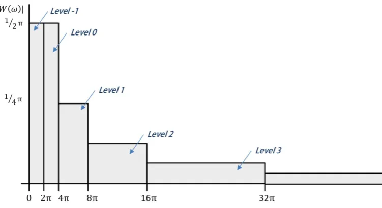
Dyadic Harmonic wavelets may be defined simply in the frequency domain from Eq.2.40 as shown in Figure 2.12.

W(ω) = ( 1 2π)2

−j

e

−iωk

2j (2.40)

The inverse Fourier transform of the frequency defined Harmonic wavelet W(ω) gives its time domain representation,

w(2jt−k) =

ei4π(2jt−k)−ei2π(2jt−k)

i2π(2j_t₋_k₎ (2.41)

at levelj and translationk. The complex form allows two real wavelets to be expressed in a single expression, much like a Fourier series. At the lowest band, j = −1, the inverse Fourier transform produces the scaling function,

ϕ(t−k) = e

i2π(t−k)₋₁

i2π(t−k) (2.42)

As previously stated, a key feature of these wavelets comes from the fact that the scaling function and each dilation set, Wj(ω) occupies its own unique, non-overlapping space

in the frequency domain. It is therefore intuitive that this family of wavelets should form an orthogonal set. The orthogonality properties of the dyadic harmonic wavelet transform are discussed in [17].

(40)

[image:40.595.87.463.72.277.2]

Figure 2.12: Dyadic harmonic wavelets in the frequency domain start-ing from Level -1

time resolution at low frequencies and low frequency, high time resolution at high fre-quencies. A generalized harmonic wavelet of (m, n) scale (bounding the wavelet in the frequency domain) and (k) position in time attains a representation in the frequency domain of the form

ΨG₍_m,n₎_,k(ω) =

(

1 (n−m)∆ωe

−iωkT0

n−m

, m∆ω ≤ω≤n∆ω

0, otherwise

, (2.43)

wherem, n and k are considered to be positive integers and ∆ω = 2_Tπ

0 , and whereT0

is the total time duration of the signal under consideration. Harmonic wavelets of the form of Eq.(2.43) span frequency bands defined by m and n as shown in Figure 2.13. An orthogonal set of harmonic wavelets are produced when n and m define adjacent non-overlapping intervals for all wavelets in the set. Asn−mnears 1, the wavelet tends towards a single harmonic (high frequency resolution); however, asn−mincreases, the wavelet becomes more compressed in the time domain and hence offers higher resolution in time (Figure 2.14). The analyst may choose a single value of m−n for the entire wavelet set, defining a fixed time-frequency resolution for the wavelet transform or vary

n−m to increase, or decrease band-dependant time-frequency resolution. The inverse Fourier transform of Eq.(2.43) gives the time-domain representation of the wavelet, which is equal to

ΨG₍_m−n₎_,k(t) = e

in∆ωt−kT0

n−m

−e

im∆ωt−kT0

n−m

i(n−m) ∆ω

t− kT0

n−m

(2.44)

Furthermore, the continuous generalized harmonic wavelet transform (GHWT) is de-fined as

W₍G_m,n₎_,k = n−m

kT0

Z ∞

−∞

f(t) ΨG₍_m,n₎_,k(t)dt, (2.45) and projects the functionf(t) on this wavelet basis.

Redundant and non-redundant harmonic wavelet transforms

(41)

[image:41.595.151.487.441.680.2]

Figure 2.13: Harmonic wavelets in the frequency domain withn−m= 8Hz

(42)

frequency band at every translationk, the circular convolution of the signal and wavelet may be computed efficiently via the FFT. Note that taking the convolution of two signals is equivalent to transforming them to the Fourier domain, multiplying them and then inverse transforming them back to the time domain. This requires significantly less computational effort than multiplying each individual time step (i.e., operations in the order ofN2 are reduced to the order of NlogN). This also does not take account of the computational time required to evaluate Eq.2.44 for which the frequency domain representation required for convolution via the FFT (Eq.2.43) is significantly simpler.

The convolution of the signalf(t) with the conjugate wavelet ΨG₍_m,n₎_,k is performed by multiplying the FFT off(t) with the band-limited frequency domain representation of the wavelet, Eq.2.43 and then performing the inverse FFT. The procedure is illus-trated in Figure 2.15. It is important to note that this scheme represents a redundant transform and does not project the source signal onto an orthogonal basis. This is be-cause for each wavelet band, there are an equal number of coefficients to the length of the signal. Hence the entire transform produces many more coefficients than the length of the signal in which the wavelet spectrum at adjacent times is highly correlated [32]. Consider that repeating the calculation in Eq.2.45 for different integer values of k is equivalent to performing a convolution of Eq.2.44 in which k= 0 with the signal f(t) in increments of T0

n−m. Then the redundant wavelet transform illustrated in Figure 2.15

is equivalent to performing Eq.2.45 atN integer values ofk(spanning the length of the signal) using the following time-domain representation of the wavelet,

ΨG₍_m−n₎_,k(t) = e

(in∆ω(t−k))₋_e(im∆ω(t−k))

i(n−m) ∆ω(t−k) . (2.46) This redundant transform has the effect of smoothing the wavelet representation of the signal along the time axis and can be useful in identifying time-dependent properties of a signal. However, it is not possible to perform an inverse wavelet transform in a redundant basis (with the aim of reproducing the same original signal) as multiple reconstructed signals would be possible from a single set of wavelet coefficients. The non-redundant form of the GHWT is revisited in Chapter 5.

2.4.4 Other non-stationary spectral analysis techniques

Harmonic wavelets are used throughout this project for a number of reasons. They present a natural, intuitive extension from Fourier analysis into the joint time-frequency domain; indeed a harmonic wavelet basis in which m−n = 1 in Eq.2.43 is identical the Fourier series. Also, the GHWT may be applied with a range of time-frequency resolution settings (i.e. variation ofn−min Eq.2.43) whilst maintaining an orthogonal basis; utilizing an orthogonal basis enables exact reconstruction of the original signal from basis coefficients. Another important point is that harmonic wavelets can be utilized to generate a spectrogram showing clear, quantifiable frequency bands rather than ‘levels’ or ‘scales’ produced by alternative wavelet bases. Finally, the GHWT was also chosen for ease of interpretation when developing missing data reconstruction methods; due to the band limited nature and orthogonal properties of the GHWT, when working with simulated data, algorithm problems and programming errors are quickly identified. This is a very useful property from a research perspective.

(43)

[image:43.595.186.454.68.317.2]

Figure 2.15: FFT algorithm for producing harmonic wavelet coeffi-cients

(including those based on the GHWT) could be utilized before applying alternative spectrum estimation methods. Example of alternative spectrum estimation techniques include:

• The Wigner-Ville method (WVM): This is an alternative approach to both wavelet and time window based non-stationary spectral estimation, named after E.P. Wigner [33] who used it first in quantum mechanics and J.Ville [34] who first proposed its use in harmonic analysis. Explanations of the method can be found in [35, 14].

• The S-transform: This can be thought of as an extension of the STFT or as a type of wavelet analysis based on windowed sinusoids [36]. Where the STFT involves repeatedly analysing the entire frequency content of a signal over a pre-defined fixed window that is moved along the time-history, the S-transform allows for variable sized time windows.

• Chirplet transforms: A chirplet is similar to a wavelet, in that it has localized energy and is oscillatory, with the difference being that its frequency content changes over time. By using an over-defined dictionary of chirplets, the adaptive chirplet transform [14] is able to capture highly non-stationary elements without needing to reduce overall frequency resolution (as would be required to detect similar elements through a standard wavelet transform).

2.5 Stationary process representation & power spectral

estimation

(44)

Z ∞

−∞

|x(t)|dt <∞ (2.47)

is not guaranteed (required for classical Fourier analysis, preventing infinite mag-nitude coefficients). Instead, the Fourier transform of the autocorrelation function is considered. This approach makes the assumption that x(t) has no lasting periodic components below some minimum frequency, and hence

RX(τ → ∞) = 0 (2.48)

The idea is that the autocorrelation function RX(τ) gives information about the

frequencies present in a random process indirectly whilst being of finite energy. The power spectrum for the processx(t) is given as

SX(ω) =

1 2π

Z ∞

−∞

RX(τ)e−iωτdτ (2.49)

The units of the power spectrum SX(ω) are those of (process variance) / (unit

of frequency), with the area under the entire curve being equal to the total process variance. However, it can be shown that the power spectrum density can be directly related to the Fourier transform of a stationary stochastic process, according to the theory of ‘generalized harmonic analysis’ [37].

For any real-valued stationary process, X(t), there exists a corresponding complex orthogonal processZ(ω), such thatX(t) can be written in the form Eq.2.50, e.g. [38, 39, 4].

X(t) =

Z ∞

−∞

eiωdZ(ω) (2.50)

Eq.2.50 is a ’stochastic integral’ in whichZ(ω) is the Fourier-Stieltjes transform ofX(t). IfZ(ω) is differentiable, then Eq.2.50 reduces to the standard inverse Fourier transform. For stationary stochastic processes, Z(ω) is an orthogonal stochastic process, i.e., for non-overlapping intervalsdω anddω0, the corresponding incrementsdZ(ω) anddZ(ω)0 are uncorrelated. The average expected power of the process within the frequency intervaldω is given by E|dZ(ω)|2_{. From this the power spectral density function may} be defined,

E dZ2(ω)

=SX(ω)dω (2.51)

and

E(dZ(ω)) = 0. (2.52)

In Eq.2.51,SX(ω) is the two-sided power spectrum of the processX(t) . Further, a

versatile formula for generating realizations compatible with the stationary stochastic process model of Eq.(2.50) is given by [1]

X(t) =

N−1

X

j=0

q

4SX(ωj) ∆ωsin (ωjt+ Φj) (2.53)