Regions
JIHUI ZHANG
Master of Engineering, Harbin Institute of Technology, China
Bachelor of Engineering, Harbin Institute of Technology, China
May 2019
A thesis submitted for the degree of Doctor of Philosophy of The Australian National University
3 6 . 6 < : , . < 0 + , 3 0 5 , : 4 ( 9 * /
; / , ( < : ; 9 ( 3 0 ( 5 5 ( ; 0 6 5 ( 3 < 5 0 = , 9 : 0 ; @
;OL(5<SVNVPZHJVU[LTWVYHY` YLÅLJ[PVUVMV\YOLYP[HNL 0[JSLHYS`WYLZLU[ZV\YUHTL V\YZOPLSKHUKV\YTV[[V! -PYZ[[VSLHYU[OLUH[\YLVM[OPUNZ ;OL(5<SVNVYLTHPUZWYVWLY[`VM[OL<UP]LYZP[`;VWYLZLY]L [OLH\[OLU[PJP[`VMV\YIYHUKPKLU[P[`[OLYLHYLY\SLZ[OH[ NV]LYUOV^V\YSVNVPZ\ZLK 7YLMLYYLKSVNV ;OLWYLMLYYLKSVNVZOV\SKIL\ZLKVUH^OP[LIHJRNYV\UK ;OPZ]LYZPVUPUJS\KLZISHJR[L_[^P[O[OLJYLZ[PU+LLW.VSKPU LP[OLY74:VY*4@2 )SHJR >OLYLJVSV\YWYPU[PUNPZUV[H]HPSHISL[OLISHJRSVNVJHU IL\ZLKVUH^OP[LIHJRNYV\UK 9L]LYZL ;OLSVNVJHUIL\ZLK^OP[LYL]LYZLKV\[VMHISHJR IHJRNYV\UKVYVJJHZPVUHSS`HUL\[YHSKHYRIHJRNYV\UK 3VNVHUKHWWYV]HSZJHUILVI[HPULKMYVTIYHUK'HU\LK\H\ +LLW.VSK *4@2 9.) 74:4L[HSSPJ 74: )SHJR *4@2 9.) 74:7YVJLZZ)SHJR 7YLMLYYLKSVNV )SHJR]LYZPVU 9L]LYZLK]LYZPVU
Any application of the ANU logo on a coloured background is subject to approval by the Marketing Office. Please send to [email protected]
(5<
3VNV<ZL.\PKLSPULZ
Research School of Engineering
The contents of this thesis are the results of original research and have not been
submitted for a higher degree to any other university or institution. Much of this
work has either been published or submitted for publications as journal papers and conference proceedings. Following is a list of these papers.
Journal Publications
• J. Zhang, T. D. Abhayapala, P. N. Samarasinghe, W. Zhang, and S. Jiang,
’Multichannel active noise control for spatially sparse noise fields’, The
Jour-nal of the Acoustical Society of America, vol. 140, no. 6, pp. EL510−EL516,
2016.
• J. Zhang, T. D. Abhayapala, W. Zhang, P. N. Samarasinghe and S. Jiang,
”Active Noise Control Over Space: A Wave Domain Approach,” inIEEE/ACM
Transactions on Audio, Speech, and Language Processing, vol. 26, no. 4, pp.
774-786, April 2018.
• J. Zhang, T. D. Abhayapala, W. Zhang, and P. N. Samarasinghe, “Active
Noise Control over Space: A Subspace Method for Performance Analysis,”
Applied Sciences, vol. 9, no. 6, pp. 1250, March 2019.
Conference Proceedings
• J. Zhang, W. Zhang, and T. D. Abhayapala, Noise cancellation over spatial
regions using adaptive wave-domain processing, in Proc. IEEE Workshop on
Applications of Signal Processing to Audio and Acoustics (WASPAA) 2015,
New Paltz, NY, USA, October 2015, pp. 1-5
• J. Zhang, T.D. Abhayapala, P. N. Samarasinghe, W. Zhang and S. Jiang, Sparse complex FxLMS for active noise cancellation over spatial regions, in
IEEE International Conference on Acoustics, Speech and Signal Processing (ICASSP), Shanghai, China, March 2016, pp. 524-528
• H. Chen, J. Zhang, P. N. Samarasinghe, and T. D. Abhayapala, Evaluation of
spatial active noise cancellation performance using spherical harmonic
analy-sis, in Proc. IEEE International Workshop on Acoustic Signal Enhancement
2016, Xi0an, China, September 2016, pp. 15.
The following papers are also results from my Ph.D. study, but not included in
this thesis:
Journal Publications
• Y. Xu, J. Zhang, Real-time detection algorithm for small space targets based
on max-median filter, Journal of Information and Computational Science,
vol. 11, no. 4, pp. 1047-1055, 2014
• Y. Xu, J. Zhang, Y. Wei, Recent patents on real-time deep space target track
system based on dual-DSP, Recent Patents on Computer Science, vol. 6, no.
3, pp. 227-232, Dec. 2013
Conference Proceedings
• Y. Xu, J. Zhang, X. Liu, The research on the design and application of a new
configurable test instrument, 2014 IEEE AUTOTESTCON, St. Louis, MO,
USA, Sep. 2014, pp. 342-345
• Y. Xu, J. Zhang, X. Liu, The research on a new implementation scheme of the
portable general purpose automatic test system, 2014 IEEE
AUTOTEST-CON, St. Louis, MO, USA, Sep. 2014, pp. 173-176
The research work presented in this thesis has been performed jointly with Prof.
Thushara D. Abhayapala, Dr. Wen Zhang, Dr. Prasanga N. Samarasinghe, and
Jihui Zhang
Research School of Engineering The Australian National University
Canberra ACT 2601
Without the support of the many faces in my life, this work would not have been
completed. I would like to acknowledge and thank each of the following.
• First and foremost, my supervisors, Prof. Thushara Abhayapala, Prof. Wen
Zhang, and Dr. Prasanga Samarasinghe, for their valuable guidance and true
friendship along my research.
Special thanks goes to Thushara, for his unconditional support and care
throughout all the difficulties.
Thanks Wen, for her detailed guidance and support since the beginning of my ANC research, along all the variations of our lives.
Thanks Prasanga, for providing many suggestions on the research and
valu-able feedback during the process of writing.
• Prof. Shouda Jiang and Dr. Yonghui Xu, my supervisors in the Harbin
Institute of Technology, China, for supporting me to study in Australia.
• The Australian National University, for the PhD opportunity,
Postgradu-ate Research Scholarship, HDR Fee Remission Merit Scholarship and many
administrative supports.
• The China Scholarship Council, for the State Scholarship.
• My friends in the Audio & Acoustic Group, the Signal Processing Group,
and the Communication Group, specially Farhana, Shama, Nicole, Hanchi,
Jing, Fahim, Katrina and Yuting, for their true friendship.
• Mr. Yuki Mitsufuji, for giving me the internship opportunity at SONY Japan.
• My parents, for their constant encouragement and inspiration.
This thesis investigates active noise control over a large spatial region using
effi-cient control systems. Active noise control (ANC) utilises secondary sound sources to cancel primary noise based on the principle of destructive interference, and has
the advantage of high flexibility and easy adaptability. ANC over a large
spa-tial region (spaspa-tial ANC), which requires multiple sensors and multiple secondary
sources in the system, creates a large-sized quiet zone for multiple listeners in
three-dimensional spaces. The existing multichannel approaches are not very efficient in
spatial ANC, as the noise cancellation is optimized only around the error sensors.
This thesis provides new adaptive solutions for spatial ANC in general noise fields
and optimal methods for spatial ANC in sparse noise fields.
In terms of adaptive solutions for spatial ANC in a general noise field, our
ap-proach is to utilize the wave-domain signal processing technique. Several outcomes
resulting from this approach are (1) the design of the feedback wave-domain ANC
system, and derivation of the filtered-x least mean square wave-domain approaches; (2) systematical formulation of the wave-domain ANC into different minimization
problems and different updating variables, and derivation of four normalized
wave-domain approaches. We show that, compared to the conventional multichannel
approaches, the proposed wave-domain ANC approaches can achieve significant
noise reduction over the entire spatial region with faster convergence speed.
In terms of the optimal methods for spatial ANC in a sparse noise field, our
approach is to incorporate the `1-norm constraint from compressive sensing into
the spatial ANC. Several outcomes resulting from this approach are (1) derivation
of the `1-constrained multichannel approaches; (2) derivation of the`1-constrained
wave-domain approach. We show that, compared to the conventional multichannel
approaches, the proposed `1-norm constrained approaches can reduce the number
of active secondary sources with faster convergence speed.
In addition, this thesis investigates the best possible spatial ANC performance
for a given system, by analyzing the signal space spanned by the secondary sources
within a given acoustic environment. The proposed subspace method can obtain
best possible ANC performance and is demonstrated to be a feasible solution, especially when the secondary sources are not sufficient to cover all orthogonal
List of Acronyms
ANC Active noise control
SNR Signal to noise ratio
ATF Acoustic transfer function
PCA Principal component analysis
3-D Three-dimensional
2-D Two-dimensional
LMS Least-mean-square
FxLMS Filtered-x least mean square algorithm
NLMS Normalized least mean square algorithm
WFS Wave field synthesis
WD Wave domain
MP Multi-point
NMP Normalized multi-point algorithm
NWD-D Normalized wave-domain algorithm updating driving signals
NWD-M Normalized wave-domain algorithm updating mode coefficients
NEWD-D Normalized energy-based wave-domain algorithm
updating driving signals
NEWD-M Normalized energy-based wave-domain algorithm
updating the mode coefficients
APE Acoustic potential energy
AED Acoustic energy density
GED Generalized acoustic energy density
C`1-MP Complex `1 constrained multi-point algorithm
S`1-MP Scalar `1 constrained multi-point algorithm
Leaky-MP Leaky multi-point algorithm
WD-FxLMS Wave-domain filtered-x least mean square algorithm
MP-FxLMS Multi-point filtered-x least mean square algorithm
`1-WD-FxLMS `1-norm constraint wave-domain FxLMS algorithm
`1-MP-FxLMS `1-norm constraint multi-point FxLMS algorithm
d·e Ceiling operator
[·]∗ Complex conjugate of a vector or matrix
[·]T Transpose of a vector or matrix
[·]H Complex conjugate transpose of a matrix
| · | Euclidean norm of a vector
k · k1 `1 Norm
k · k2 `2 Norm
∗ Linear convolution
A−1 Matrix inverse
A† Matrix pseudoinverse
x·y Dot product between two vectors
E{·} Expectation operator
<{·} Real part
={·} Imaginary part
δ{·} Dirac delta function
δum{·} Kronecker delta function
exp{·} Exponential function
H0(2)(·) Zeroth-order Hankel function of the second kind
Jm(·) Bessel function
Yum(·) Spherical harmonics
∇(·) Gradient
<·> the dot product of two vectors
i √−1
k Wave number
c Speed of sound propagation
ρ0 Density of the media
M Wave domain mode after truncation
n Iteration number of the adaptation
u Spherical harmonics order
m Number of spherical harmonics basis of each order
xin Reference input of the FxLMS algoirthm
ω Adaptive filter
r Radius of arbitrary point with respect to origin
φ Azimuthal angle
∆φ Angles between two loudspeakers
p Sound pressure on the arbitrary points
ψ Polar angle (elevation angle)
x Any arbitrary point inside the interest region
w Angular frequency
y Loudspeaker position
e Residual noise field
α Residual noise field coefficients in wave domain
P Average energy of the residual signal over the entire region
v Primary noise field
β Primary noise field coefficients in wave domain
s Secondary noise field
γ Secondary noise field coefficients in wave domain
d Loudspeaker weights
G Acoustic transfer function
T Acoustic transfer function coefficients in wave domain
ξ Cost function
ω Update variable
µ Step size
ρ Leakage factor
δ Sparsity level (for `0 constraint)
λ Sparsity parameter (for `1 constraint)
θ Phases of complex driving signals
L Loudspeaker number
Q Microphone number
Z Number of evaluation point inside the interest region
R1 Radius of the interest region
R2 Radius of the loudspeaker array
Rz Radius of the microphone array
χ Continuance loudspeaker distribution
τ Continuance loudspeaker distribution in wave domain
σ ATF for continuance loudspeaker array
U Acoustic potential energy weights
κ Loudspeaker coefficients in the subspace
Loudspeaker vector composed by eigenvalues and eigenfunctions
O Basis of the subspace
Nrin Noise reduction inside the region of interest
Declaration i
Acknowledgements v
Abstract vii
List of Acronyms ix
Notations and Symbols xiii
Contents xvii
List of Figures xxi
List of Tables xxvii
1 Introduction 1
1.1 Motivation and Scope . . . 1
1.2 Problem Description . . . 5
1.3 Thesis Outline . . . 6
2 Literature Review and Background Theory 11 2.1 Single-channel ANC Techniques . . . 11
2.1.1 Feed-forward control system . . . 12
2.1.2 Feedback control system . . . 16
2.2 Multichannel ANC Techniques . . . 17
2.2.1 Multichannel algorithm and variation . . . 18
2.2.2 Global ANC using multichannel algorithms . . . 20
2.2.3 Regional ANC using multichannel algorithms . . . 22
2.3 Wave-domain Sound Field Representation . . . 22
2.3.1 Sound field and acoustic environment in a space . . . 24
2.3.2 Wave-domain expansion of a sound field . . . 28
2.4 Summary . . . 33
3 Multiple-point ANC for Directional Sparse Noise Fields 35 3.1 Introduction . . . 35
3.2 Spatial ANC Problem Formulation . . . 37
3.3 Conventional Multi-point Algorithms . . . 39
3.3.1 Multi-point algorithm . . . 39
3.3.2 Leaky multi-point algorithm . . . 40
3.4 Sparsity Constrained Multi-point Algorithms . . . 41
3.4.1 `0-norm constrained multi-point algorithm . . . 41
3.4.2 Complex `1-norm constrained multi-point algorithm . . . 42
3.4.3 Scalar `1-norm constrained multi-point algorithm . . . 44
3.5 Parameter Selection . . . 45
3.6 Simulation Results . . . 46
3.6.1 Single primary source scenario . . . 48
3.6.2 Multiple primary source scenario . . . 52
3.7 Summary and Contributions . . . 53
3.8 Related Publications . . . 53
4 Wave Domain ANC: Basic Structure 55 4.1 Introduction . . . 56
4.2 Wave Domain ANC Formulation . . . 57
4.2.1 Primary noise field . . . 58
4.2.2 Secondary sound field . . . 58
4.2.3 Residual signals . . . 61
4.2.4 Wave-domain ANC . . . 62
4.3 Wave-domain FxLMS Algorithm . . . 62
4.5 Simulation Results . . . 67
4.5.1 Single-frequency noise field . . . 69
4.5.2 Multi-frequency noise field . . . 74
4.6 Summary and Contributions . . . 76
4.7 Related Publications . . . 78
5 Wave Domain ANC: Different Cost Functions and Adaptations 79 5.1 Introduction . . . 79
5.2 Problem Formulation . . . 81
5.2.1 System model . . . 81
5.2.2 Multichannel wave-domain active noise control . . . 82
5.3 Wave Domain ANC Algorithms - Minimization of Squared Residual Signal Coefficients . . . 83
5.3.1 Normalized wave-domain algorithm updating driving signals (NWD-D) . . . 84
5.3.2 Normalized wave-domain algorithm updating mode coeffi-cients (NWD-M) . . . 85
5.4 Wave Domain ANC Algorithms - Minimization of Acoustic Potential Energy . . . 86
5.4.1 Normalized energy-based wave domain algorithm updating driving signals (NEWD-D) . . . 88
5.4.2 Normalized energy-based wave domain algorithm updating mode coefficients (NEWD-M) . . . 88
5.5 Simulation Results Analysis . . . 89
5.5.1 Simulation setup . . . 89
5.5.2 Single frequency scenario . . . 92
5.5.3 Multi-frequency scenario . . . 100
5.6 Summary and Contributions . . . 102
5.7 Related Publications . . . 105
5.8 Appendices . . . 105
5.8.1 Proof of equation (5.10) . . . 105
5.8.2 Proof of equation (5.13) . . . 106
5.8.4 Proof of equation (5.24) . . . 107
6 ANC Subspace Performance Analysis 109
6.1 Introduction . . . 110
6.2 Problem Formulation . . . 111
6.3 Wave-domain Least Square Method . . . 114
6.4 Subspace Method . . . 116
6.4.1 Principal component analysis of the secondary path . . . . 116
6.4.2 Projection from the primary sound field into the subspace . 118
6.4.3 Noise control in the subspace . . . 119
6.5 Simulation Results . . . 120
6.5.1 Simulation setup . . . 122
6.5.2 Cancellation performance using different methods . . . 125
6.5.3 Comparison of the effect of different noise source positions . 128
6.5.4 Comparison of the effect of different loudspeaker placements 128
6.6 Summary and Contributions . . . 131
6.7 Related Publications . . . 134
7 Conclusion and Future Research Directions 135
7.1 Conclusions . . . 135
7.2 Future Work . . . 138
1.1 Passive noise control and active noise control [1]. . . 2
1.2 Basic ANC system structure. . . 3
1.3 An example of shared office space with personal sound zones for each
individual [2]. . . 4
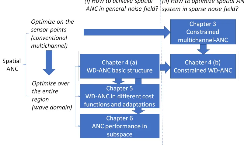
1.4 Breakdown of the spatial ANC problem into each chapter. WD-ANC
denotes the wave-domain ANC. . . 7
2.1 Fundamental components in a feed-forward ANC system. . . 12
2.2 Block diagram of feedforward ANC using LMS algorithm, where
xin(n) is the input reference signal,v(n) is the primary signal on the
error microphone position, e(n) is the error signal, and d(n) is the
driving signal. . . 13
2.3 Block diagram of FxLMS feed-forward ANC. . . 15
2.4 Single-channel feedback ANC system. . . 17
2.5 Block diagram of multichannel feedforward ANC system, where Pr
is the primary path from reference sensors to error sensors,GandGb
represent the secondary path and the estimation of secondary path,
respectively. . . 18
2.6 An arbitrary point in Cartesian coordinates and polar coordinates
in 2-D space. . . 23
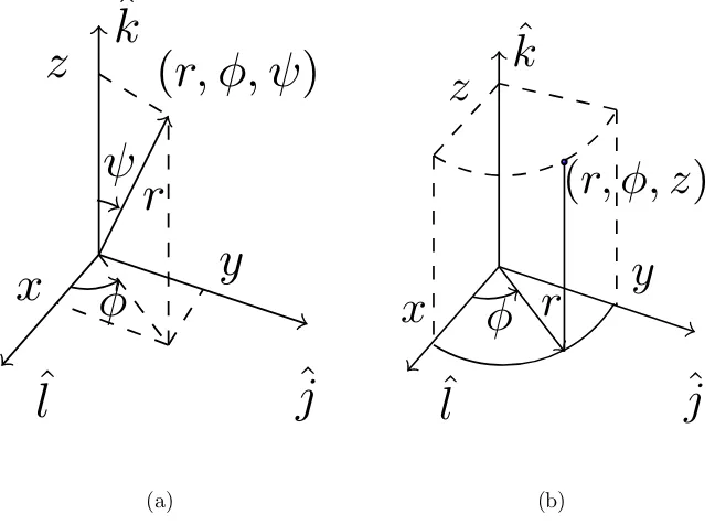
2.7 Coordinate system in 3D space: (a) Cartesian coordinates and
spher-ical coordinates; (b) Cylindrspher-ical coordinates. . . 25
2.8 Interior sound field. The stars are positions of the noise sources. . . 27
3.1 ANC setup with a circular region of interest and the block diagram
of the multi-point feedback ANC system. . . 37
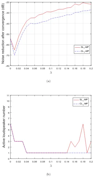
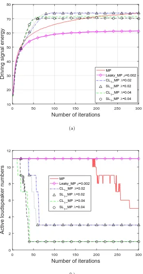
3.2 Noise reduction and active loudspeaker number after convergence
using the `1-norm constrained ANC algorithm for different value
of λ. (a) Noise reduction over the region, (b) Active loudspeaker
numbers. . . 47
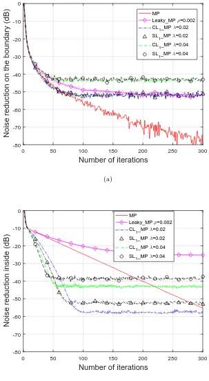
3.3 Comparison of the convergence speed and noise reduction level
us-ing different ANC algorithms, when the primary sound field is
con-structed by a primary source: (a) noise reduction on the boundary,
(b) noise reduction inside the region. . . 49
3.4 Comparison of the loudspeakers using different ANC algorithms,
when the primary sound field is constructed by a primary source:
(a) loudspeaker driving signal energy for each iteration, (b) active
loudspeaker numbers for each iteration. . . 51
4.1 A spatial ANC region (blue) consists of a circular microphone array
of radius R1 and a circular loudspeaker array of radius R2. . . 57
4.2 Block diagram of the wave-domain FxLMS algorithm for ANC. Blocks
of Tr and Tr−1 represent the wave-domain transform and the inverse
wave-domain transform, respectively. . . 64
4.3 The results of ANC in the free-field. The inner array is the
micro-phone array, outer array is the loudspeaker array. (a) The energy of
the initial noise field. (b) The residual energy after 30 iterations of
WD-FxLMS. (c) The residual energy after 30 iterations of MP-FxLMS. 68
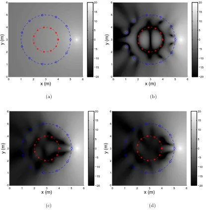
4.4 The results of ANC in the free-field. The inner array is a microphone
array and the outer array is a loudspeaker array. (a) The energy of
the initial sparse noise field. The residual energy after 30 iterations
of (b) MP-FxLMS, (c) `1-MP-FxLMS, and (d) `1-WD-FxLMS. . . 70
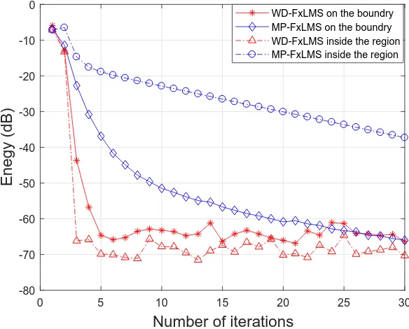
4.5 Comparison of convergence performance for noise cancellation using
WD-FxLMS and MP-FxLMS algorithm in the free-field in the first
30 iterations. . . 71
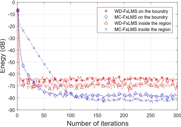
4.6 Comparison of noise cancellation after convergence using WD-FxLMS
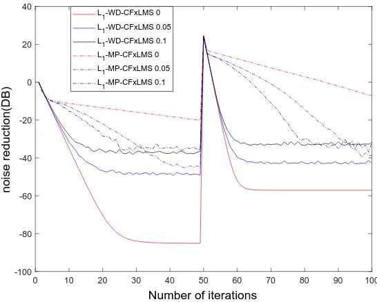
4.7 Comparison of convergence performance for noise cancellation using
`1-WD-CFxLMS and`1-MP-CFxLMS algorithms with variable zero
attractor strength (λ = 0,0.05,0.1). . . 73
4.8 Comparison of convergence performance for `1-norm of the
loud-speaker weights using `1-WD-CFxLMS and `1-MP-CFxLMS
algo-rithms with variable zero attractor strength (λ= 0,0.05,0.1). . . 73
4.9 Results of ANC in reverberant environment. The inner and outer
arrays are microphone array and loudspeaker array, respectively. (a)
The energy of the initial noise field. The residual energy after 30
iterations of (b) WD-FxLMS, and (c) MP-FxLMS. . . 75
4.10 Comparison of convergence performance for noise cancellation using
WD-FxLMS and MP-FxLMS algorithm in reverberant environment. 76
4.11 Noise reduction using WD-FxLMS algorithm after 30 iterations in
multi-frequency noise field. . . 77
5.1 A spatial ANC region (blue) consists of a circular microphone array
of radius R1 and a circular loudspeaker array of radius R2. . . 81
5.2 Block diagram of wave-domain ANC system, when updating the
loudspeaker driving signals. The WD transform block represents
the wave-domain transform for the residual signals. . . 84
5.3 Block diagram of wave-domain ANC system, when updating the
wave-domain coefficients. The WD transform block represents the
wave domain transform for the residual signals. . . 86
5.4 Noise cancellation performance after 50 iterations using different
ANC algorithms in free field: (a) Primary noise field (200 Hz) (b)
Normalized MP (c) NWD-M (d) NWD-D (e) NEWD-M (f) NEWD-D. 91
5.5 Noise cancellation performance after 50 iterations using different
ANC algorithms in reverberant environments: (a) primary noise field
(200 Hz) (b)Normalized MP (c) NWD-M (d) NWD-D (e) NEWD-M
(f) NEWD-D. . . 93
5.6 Convergence performance using different ANC algorithm in free field
(50 iterations): (a) Nb
r(n) (b) Nrin(n) (c) APE reduction over the
5.7 Convergence performance using different ANC algorithm in free field
(500 iterations): (a) Nrb(n) (b) Nrin(n) (c) APE reduction over the
region. . . 95
5.8 Convergence performance in reverberant environment (50 iterations):
(a) Nb
r(n) (b) Nrin(n) (c) APE reduction over the region. . . 96
5.9 Convergence performance in reverberant environment (1000
itera-tions): (a) Nb
r(n) (b) Nrin(n) (c) APE reduction over the region. . . 97
5.10 Convergence performance using 9 loudspeakers in reverberant
envi-ronment (1000 iterations): (a) noise reduction inside the region (b)
acoustic potential energy reduction over the region. . . 99
5.11 Loudspeaker energy (dTd) using different ANC algorithms during
1000 iterations in reverberant environment: (a) 11 loudspeakers (b)
9 loudspeakers. . . 101
5.12 Multi-frequency performance using different wave-domain ANC
al-gorithms in free field after 50 iterations: (a) noise reduction within
the region (b) acoustic potential energy reduction over the region. . 103
5.13 Multi-frequency performance using different wave-domain ANC
al-gorithms in reverberant environment after 50 iterations: (a) noise
reduction within the region (b) acoustic potential energy reduction
over the region. . . 104
6.1 ANC system in a 3-D room. . . 111
6.2 ANC system setup, where the pink point is the noise source position,
blue points are loudspeaker positions, and red points are microphone
positions: (a) case 1; (b) case 2. . . 121
6.3 Energy of the primary noise field, where pink point is the projection
of the primary source on the x-y plane, blue points are the
loud-speaker points located on the x-y plane, and the red dashed circle is
6.4 Energy of the residual noise field, when the noise field is generated
by one primary source using different methods. Here, pink point
is the projection of the primary source on the x-y plane and blue points are the loudspeaker points located on the x-y plane: (a) the
WDLS method in case 1; (b) the WDLS method in case 2; (c) the
subspace method in case 1; (d) the subspace method in case 2. . . . 126
6.5 Two different array setups, when the noise source moves around a
sphere, where in both setups, pink points are the primary source
positions, blue points are loudspeaker positions, and red points are
microphone positions: (a) Case 3; (b) Case 4. . . 127
6.6 Noise reduction performance in case 3, when the noise field is
gener-ated by one primary source moving around the sphere using differ-ent methods: (a) with SNR = 60 dB white noise on the microphone
recordings; (b) with SNR = 30 dB white noise on the microphone
recordings. . . 129
6.7 Energy of the driving signals in case 3, when the noise field is
gener-ated by one primary source moving around the sphere using
differ-ent methods: (a) with SNR = 60 dB white noise on the microphone
recordings; (b) with SNR = 30 dB white noise on the microphone
recordings. . . 130
6.8 Noise reduction over the region using different loudspeaker setups,
when the noise field generated by one primary source moving around
the sphere using different methods: (a) case 3; (b) case 4. . . 132
6.9 Energy of the driving signals generated by one primary source
mov-ing around the sphere usmov-ing different methods: (a) case 3; (b) case
4. . . 133
7.1 Conclusion and future works for spatial ANC over region. The blue
blocks represent the works have been done in this thesis, and the
3.1 Noise reduction on the boundary, noise reduction inside the
re-gion, and active loudspeaker numbers after convergence in different
frequency bins using different ANC algorithms, when the primary
sound field is constructed by a primary source. . . 50
3.2 Noise reduction inside the region and active loudspeaker numbers
after convergence in different source locations, when the primary
sound field is constructed by two primary sources. . . 52
5.1 Attenuation level using different numbers of loudspeakers. . . 100
6.1 Loudspeaker array setup and noise source location in each case. . . 123
6.2 Loudspeaker positions for non-symmetric placement and symmetric
placement. . . 123
Introduction
1.1
Motivation and Scope
Acoustic noise is a common disturbance throughout our daily life. For example,
when reading this thesis, you may hear a wide range of noises which distract your
attention, such as noise from a construction site across the road, or a door slammed
by a colleague as they leave. As the amount of industrial equipment increases, such as engines, blowers, fans, transformers, noise problems become more and more
evident [3]. Excessive amounts of acoustic noise above a certain level are the main
cause of hearing loss, which drastically reduces the quality of life [4]. This thesis
is focused on finding ways of reducing acoustic noises to improve our lives.
Noise control, or noise cancellation, is designed to control the noise we hear, to
minimize the ‘residual noise’ after the cancellation process. There are two methods
of controlling noise, passive noise control and active noise control (ANC), as shown
in Figure 1.1.
One noise control method is passive noise control, in which noise-isolating
ma-terials and acoustic structures are applied to attenuate noise [5]. Example of
noise-isolating materials includes insulation, sound-absorbing tiles, and mufflers. Passive
noise control capability is achieved through a range of different variables including
frequency of sound, material type, material thickness, and geometry of the material.
When the wavelength of the sound is thicker than the material, it is difficult for
the material to absorb the sound [6]. Passive noise control is more effective at mid
Figure 1.1: Passive noise control and active noise control [1].
and high frequency ranges, but it is less effective in the low frequency range1 [8].
The second method used to control noise is active noise control (ANC). In
ANC systems, the noise to be cancelled is called ‘primary noise’. The system uses
‘secondary sound sources’ to generate ‘anti-noise signals’ to reduce the primary
noise. This is achieved through the principle of destructive interference [9, 10, 11].
ANC has the advantages of high flexibility and easy adaptability and over the last
30 years has become a well-researched topic. ANC has many applications, such as
noise cancelling headphones [12, 13], noise control in industrial machines [14] and
in-car noise cancellation [15,16,17,18,19]. Unlike the passive noise control strategy, ANC works better in the low frequencies [20]. Low frequency noise is dominant in
many real-world scenarios, e.g., air-conditioning noise, vehicle engine noise [21, 19]
and wind noise [18]. In this thesis, we apply the ANC technique to cancel low
frequency noise over a spatial region.
As typical noise sources and acoustic environments are always time-varying
and unknown, adaptive systems are commonly applied to iteratively calculate
sec-ondary source driving signals2. Adaptive systems are in either feed-forward or
feedback control configurations, depending on with or without reference sensors.
1Low frequency range is typically between 20 Hz to 500 Hz [7].
Figure 1.2: Basic ANC system structure.
Feed-forward configuration uses a reference sensor and an error sensor, as shown in
Figure 1.2 [22], while the feedback configuration only uses an error sensor. Hybrid
systems, a combination of feed-forward and feedback control structures, are also
used in ANC applications. In the ANC controller, some well-known algorithms
for implementation include the least-mean-square (LMS) method or its variants,
such as filtered-x LMS (FxLMS), adjoint LMS and recursive LMS [23]. The details
of feed-forward/feedback ANC structures and algorithms are given in Chapter 2,
Section 1.
There is a growing research interest in creating a large quiet zone for multiple
listeners in three-dimensional (3-D) spaces, such as noise cancellation in aircrafts
[24] and automobiles [17, 25, 18, 26]. In these applications, the control zones of
interest are large, and there are requirements for noise cancellation over the entire
region, instead of at spatial points. When people sit around a particular region,
such as around a desk in Figure 1.3, or when there are several people all requiring a
noise-free acoustic environment, noise cancellation is required to cover the relevant
spatial region. Meanwhile, ANC throughout a spatial region enables listeners to move freely within the region. Therefore, in this thesis, we investigate ANC over a
spatially extended region, which is termed as ‘Spatial ANC’.
In spatial ANC applications, multichannel ANC systems equipped with multiple
Figure 1.3: An example of shared office space with personal sound zones for each individual [2].
sensors are placed to measure the residual signals and multiple secondary sources
are utilized to generate the anti-noise signals. In the feed-forward control system,
additional reference sensors are placed to measure the primary noise. Both
time-domain [28, 29] and frequency-time-domain [30, 31] algorithms have been implemented
in multichannel ANC systems. For example, the frequency domain multichannel ANC [32] and its variations (such as Leaky ANC [33]) are now widely developed for
noise cancellation at error sensor positions and their close surroundings [31]. The
details of multichannel ANC algorithms and applications are reviewed in Chapter
2, Section 2.
The multichannel method is not very efficient in spatial noise control over a
re-gion, as the noise cancellation is optimized only on the error sensors. One method
for solving this problem is to increase the number of sensors so as to cover more
space, which dramatically increases the cost of the ANC system. More efficient
spatial sound field control and sound reproduction techniques can be applied to
address spatial ANC problems including wave field synthesis (WFS) and
spheri-cal/cylindrical harmonic based wave domain processing.
Wave field synthesis, introduced by Berkhout [34, 35], is one of the spatial
spatial ANC. WFS uses a holographic technique to reproduce a desired sound field
over a large area with a relatively large number of loudspeakers [36]. The WFS
approach is based on the Kirchhoff-Helmholtz integral [37, 38, 39]. In theory, WFS uses continuous distribution of appropriately driven secondary sources arranged on
the boundary of the desired listening area to reproduce a virtual sound field [37].
This technique has already been applied in ANC applications [40, 41]. However,
WFS-based spatial sound control has the disadvantage of requiring many secondary
sources to approximate the continuous distribution on the boundary of the desired
listening area, which is not always practical to implement for noise cancellation
over the region of interest.
Spherical/cylindrical Harmonic based wave domain processing [42] is another spatial sound field control and sound reproduction technique, which can be
ap-plied to spatial ANC. This method transfers the measurements into a
spheri-cal/cylindrical harmonic domain [43, 44, 45], and controls the entire spatial region
by manipulating the spherical/cylindrical harmonic coefficients. This technique
does not require secondary sources to be placed on the boundary of the region,
and can therefore be more feasible. The details of wave domain sound field
rep-resentation are reviewed in Chapter 2, Section 3. Up untill the beginning of this
research, Spherical/cylindrical Harmonic based wave domain processing had not
been applied to spatial ANC.
From the foregoing discussion, the key question which drives this thesis is as
follows:
How can we achieve ANC over a large spatial region using efficient
control systems?
1.2
Problem Description
We elaborate this problem into two further questions:
(i) How to achieve ANC over a large continuous region in a general noise field3?
3Here, general noise field includes free field and reverberant field, diffuse noise field and
(ii) How to exploit the sparse characteristics in a specific noise field, and based
on which to optimize the spatial ANC system?
For Question (i), we develop an ANC system to cancel the noise over a desig-nated region of space. To achieve ANC in a large continuous region, the control
objective should be the sound field over the entire region rather than multiple
observation points within the region. The generic solution can be applied to a
general noise field, regardless of the acoustic environment and the features of the
primary sources. In the ANC system over a region, secondary source placement
and adaptive algorithms are two critical factors to be investigated. Noise
cancel-lation performance for a given secondary source arrangement is also important to
ANC system design in real implementations.
For Question (ii), we optimize the spatial ANC system in directional sparse
noise fields. In noise fields which have directional sparse features, noise sources are sparsely distributed in space, and are located in one or a few directions with
respect to the origin of the region. As in general noise field, spatial ANC systems
require large numbers of secondary sources and high computational complexity, the
problem in the directional sparse noise field becomes:
How to reduce the number of secondary sources in the array, and how to reduce
the computational complexity of the algorithms?
1.3
Thesis Outline
Motivated by the above problems, in this thesis, we develop adaptive solutions for
spatial ANC within a continuous region. As shown in Figure 1.4, we investigate
the spatial ANC in general noise field, as well as in sparse noise field.
For noise cancellation in a general noise field, we (1) formulate the problem in the wave domain based on cylindrical harmonics or spherical harmonics) to achieve
ANC over large continuous regions, and propose the wave-domain ANC algorithms;
(2) investigate wave-domain ANC in different cost functions and adaptations; and
(3) derive a subspace to represent the secondary sources and the acoustic
environ-ment, and evaluate the ANC performance in this subspace.
For noise cancellation in a sparse noise field, we exploit sparse features, and
multichan-Figure 1.4: Breakdown of the spatial ANC problem into each chapter. WD-ANC denotes the wave-domain ANC.
nel ANC structure and the proposed wave-domain ANC structure to reduce the
number of secondary sources in the array and the computational complexity in the algorithms.
The performance of the proposed systems and techniques are verified through
numerical simulations.
The structure of the thesis is as follows:
Chapter 2: Literature Review and Background Theory
In Chapter 2, we review the literature on ANC methods and the wave domain
noise field control technique. We first review the single-channel ANC method. In terms of the control structure, we review the feed-forward and feed-back
configu-rations. In terms of the adaptive control, we review LMS, FxLMS, and normalized
LMS (NLMS) algorithms. Thereafter, we review the multichannel ANC algorithm
and different applications. We review the classical multichannel algorithm, and
then discuss the variations in global ANC applications and regional ANC
applica-tions. The classical multi-point algorithm which is commonly used for solution of
[image:37.595.119.520.112.351.2]new algorithms. We also study typical sound fields and the wave domain sound
field representation. The theory and methods reviewed in this chapter form the
fundamentals of my thesis.
Chapter 3: Multiple-point ANC for Directional Sparse Fields
In Chapter 3, we address question (ii) and investigate the noise control over
a region using a multichannel ANC framework in a directional sparse noise field.
We first review the conventional multi-point algorithm and Leaky multi-point
algo-rithm using the feedback control structure. Thereafter, we introduce the `1-norm
penalty to the multi-point algorithm, resulting in the complex`1-norm constrained
multi-point (C`1-MP) algorithm and the scalar `1-norm constrained multi-point
(S`1-MP) algorithm. In this chapter, driving signals of the secondary sources are
designed by minimizing the addition of a squared residual noise field and `1 norm
of the driving signal magnitude. We conduct simulations for spatial ANC
appli-cations while the noise sources are coming from a few directions. The simulation
results indicate that when the noise field has directional sparsity, the proposedC`1
-MP algorithm and proposed S`1-MP algorithm can reduce the number of active
secondary sources, with reasonable noise reduction performance.
Chapter 4: Wave Domain ANC: Basic Structure
The conventional multi-point algorithm and variations are not efficient in ANC
over a large continuous region. In Chapter 4, we apply a wave-domain signal
processing technique to spatial ANC applications. To addresses question (i), after
representing all the variables in the control system into wave-domain coefficients,
we propose a wave-domain FxLMS algorithm. Using this algorithm, we control
the noise field over the entire region directly. This results in significant noise
reduction with fast convergence speed. This advantage is evaluated in both free
field and reverberant environments. To address question (ii), we also propose the`1
-constrained wave-domain FxLMS algorithm, by introducing the `1-norm penalty
into the wave-domain ANC. This can be applied to spatial ANC in directional sparse noise fields.
Chapter 5: Wave Domain ANC: Different Cost Functions and
Adapta-tions
In this chapter, we further address question (i) and investigate the wave-domain
in terms of the wave domain residual signal coefficients. We implement normalized
LMS adaptive algorithms in the wave domain by solving two minimization
algo-rithms: (i) minimizing the squared wave-domain residual signal coefficients, and (ii) minimizing the acoustic potential energy. For each minimization problem, we
derive the update equations with respect to two variables: (i) updating the
driv-ing signals, and (ii) updatdriv-ing the wave-domain coefficients. This results in four
different wave domain algorithms (i) normalized wave domain algorithm updating
driving signals (NWD-D), (ii) normalized wave domain algorithm updating mode
coefficients (NWD-M), (iii) normalized energy-based wave domain algorithm
up-dating driving signals (NEWD-D), and (iv) normalized energy-based wave domain
algorithm updating mode coefficients (NEWD-M). We compare the four proposed
algorithms as well as the conventional multi-point algorithms in the simulation section. We evaluate these five algorithms using three criteria: acoustic potential
energy reduction, convergence speed, and energy of the secondary-source driving
signals. These numerical simulations are conducted in the free field, as well as in
the reverberant environment.
Chapter 6: ANC Subspace Performance Analysis
In Chapter 6, we investigate the noise control performance in any 3-D
reverber-ant environment. We discuss a wave-domain least square method, which matches
the primary noise field coefficients to the secondary noise field coefficients in the
wave domain. Based on the wave-domain coefficients of the acoustic transfer func-tion between loudspeakers and the control region, we derive the subspace
repre-senting the secondary sources and the acoustic environment. We then propose a
subspace method by matching the projection of the primary noise field coefficients
to the secondary noise field coefficients in the subspace. We conduct the
simula-tions to compare the proposed subspace method with the wave-domain least square
method. We compare the ANC performance under different noise source positions
and different loudspeaker configurations.
Chapter 7: Conclusion and Future Research Directions
Literature Review and
Background Theory
Overview: This chapter provides a brief overview of the background
knowledge concerning spatial ANC over a region. We first review
conventional single-channel active noise control structures, and then
focus on the use of multichannel active noise control techniques for
3-D noise field control. Furthermore, we discuss the sound field and
acoustic environment considered in this thesis. To further develop
the spatial ANC strategies in the later chapters, we review the basic
formulation of harmonics-based sound field representation. The theory
and methods reviewed in this chapter form the foundation for the rest
of the thesis.
2.1
Single-channel ANC Techniques
In ANC systems, noise sources are unknown and acoustic environments are
time-varying. Therefore, adaptive filters are employed to produce anti-noise signals. The
control structure of ANC can be broadly classified into two classes: feed-forward
control and feedback control. We review the basis of both theories and structures
in the next two subsections. The basic formulations we mentioned here can be
extended to multichannel cases as well.
2.1.1
Feed-forward control system
The feed-forward ANC scheme requires a reference signal as an input to the
adap-tive filter. This scheme is widely used for industrial applications such as reducing
duct noises [46].
The objective of feed-forward ANC is to design the driving signal of the
sec-ondary source, using sound measurements captured by a reference sensor and an
error sensor. The fundamental block diagram of a feed-forward ANC system is
shown in Figure 2.1. Here, the ANC system consists of an error sensor, a reference
Figure 2.1: Fundamental components in a feed-forward ANC system.
sensor, a secondary source, and an adaptive algorithm. Here, we assume that there
is no acoustic feedback from the secondary source to the reference sensor 1.
Some well-known adaptive algorithms used to implement feed-forward ANC
include the least-mean-square (LMS) method or its variants, such as FxLMS [47],
NLMS [48], adjoint LMS [49] and recursive LMS [33]. LMS algorithms are a class
of adaptive algorithms, which minimize the least mean squares of the error signal.
In the following subsections, we review the LMS algorithm, FxLMS algorithm and
NLMS algorithm. Here, we introduce the secondary-path transfer function G(n)
into each algorithm.
1There are several solutions to eliminate the acoustic feedback. One solution is to use a
LMS algorithm
Figure 2.2: Block diagram of feedforward ANC using LMS algorithm, wherexin(n)
is the input reference signal, v(n) is the primary signal on the error microphone
position, e(n) is the error signal, and d(n) is the driving signal.
The block diagram of a single-channel feed-forward ANC system using LMS
algorithm is shown in Figure 2.2. In this system, the controller is the adaptive filter
using the LMS algorithm. The adaptive filter ω continuously tracks variations in
the primary noise field.
In the LMS algorithm, the error signale(·) for each iteration can be written by
e(n) = v(n) +G(n)∗d(n), (2.1)
where n is the iteration number, G(·) is the impulse response of secondary path
from the secondary source to the error sensor,v(·) is the primary noise field at the
error sensor, and
d(n) =xin(n)∗ω(n), (2.2)
is the driving signal of the secondary source.
Here, ∗ denotes linear convolution, ω(n) = [ω0(n), ω1(n), ..., ωLω−1(n)]T are the
1)]T are the input reference signal.
Minimizing the mean square of the error signal, the cost function becomes
ξ(n) =e2(n). (2.3)
Since the LMS algorithm is based on the steepest descent method, the update
equation is as follows,
ω(n+ 1) =ω(n)− µ
2∇ξ(n), (2.4)
where µis the adaptation step size, and ∇is the gradient operator.
From (2.1) and (2.3), the gradient of the cost function with respect to the filter
coefficients ω is written as
∇ξ(n) = ∇(e2(n))
= 2e(n)∇e(n)
= 2e(n)x0in(n), (2.5)
where
x0in(n) = G(n)∗xin(n). (2.6)
Substituting (2.5) into (2.4), the final update equation of the LMS algorithm is written as
ω(n+ 1) =ω(n)−µx0in(n)e(n). (2.7)
In (2.7), the filter coefficients ω in the next iteration are based on the error signal
and the filtered reference signal on the current iteration, by finding the gradient of
the mean square error.
The step sizeµin (2.7) controls the convergence speed of the adaptive process,
which should be chosen properly based on the individual scenario. The upper
bound of the step size µ is given as follows [50],
µ < 2 λmax
in
, (2.8)
reference signal E{xin(n)xHin(n)}.
FxLMS algorithm
The performance of an ANC system depends largely on the secondary-path transfer
functionG[3]. In the LMS algorithm, however, due to the secondary-path transfer
function, the error signal and the reference signal are not aligned in time. This
effect will generally cause instability [51].
One effective solution to compensate for the effect of the secondary-path is to
add an identical filter on the reference signal path, which is called the FxLMS
algorithm. The block diagram is illustrated in Figure 2.3. Compared with Figure
2.2, the reference signal is filtered by the estimation of the secondary path Gb,
before being used in the LMS filter. This is the main difference between the LMS
algorithm and the FxLMS algorithm.
Figure 2.3: Block diagram of FxLMS feed-forward ANC.
Therefore, the update equation of FxLMS algorithm can be written as:
where x0in(n) is the filtered reference signal, and
x0in(n) = xin(n)∗Gb(n). (2.10)
FxLMS is very tolerant of error between the secondary path G and the
es-timation filter Gb, which can be estimated using the off-line model during initial
training in most ANC applications [3]. Adaptive online secondary path modelling
has also been applied [52, 53]. Variations of the FxLMS algorithm exist, such as
the Leaky FxLMS [54, 55] and the filtered-x normalized LMS algorithm [32], which
are proposed to improve the performance of the FxLMS.
NLMS algorithm
The normalized LMS algorithm also minimizes the mean square error, with the
same cost function as LMS algorithm. The normalization term is according to the
energy of the reference input signal xin(n). The step size in LMS algorithm has
been modified to a data-dependent step size a+kxµ in(n)k22
.
Therefore, the update equation of the NLMS algorithm is given by:
ω(n+ 1) =ω(n)− µ
a+kxin(n)k22
x0in(n)e(n), (2.11)
where k · k2 denotes the`2 norm, and a >0 is a constant to overcome the possible
numerical difficulties when kxin(n)k22 is very close to zero.
The algorithm is stable for 0 < µ < 2. Like the LMS algorithm, the next
iteration of the NLMS algorithm is based on the error signal and the filtered
refer-ence signal on the current iteration. Compared to the LMS algorithm, the NLMS
algorithm has superior robustness [56].
2.1.2
Feedback control system
In the feed-forward control system described in Section 2.1.1, we assume that there
is no acoustic feedback from the secondary source to the reference sensor.
Unfor-tunately, in some applications, the upstream sound field from the secondary source
solution is to model the acoustic feedback transfer function and incorporate it into
the system with a separate feedback cancellation filter [23]. Another solution is to
utilize the feedback structure, which is reviewed as follows.
In the feedback ANC system, only an error sensor (error microphone) and a
secondary source (loudspeaker) are utilised [57], as shown in Figure 2.4. The active
noise controller attempts to cancel the noise without the benefit of reference input.
There have been growing interests in implementing the feedback system as it avoids
the need for separate reference sensors to measure the primary noise [58]. This
reduces the number of system components and associated hardware. In particular,
it is more cost-effective and more suitable for use in large 3-D acoustic environments
with multiple noise sources [59]. However, in most cases, feedback control system
is only effective for dealing with narrowband noise.
Figure 2.4: Single-channel feedback ANC system.
2.2
Multichannel ANC Techniques
As discussed in Section 2.1, the single-channel configuration, with one error sensor and one secondary source, is well suited for both narrowband and broadband
can-cellation in narrow ducts or small areas. When the noise field is monitored at a
specific spatial point by an error sensor, noise cancellation can be achieved around
the error sensor with the spatial limit being approximatelyλmax/10 [31], whereλmax
is the wavelength of the highest undesired frequency. However, the single-channel
system is clearly insufficient for more complex enclosures or large dimension
single-channel ANC systems to multichannel ANC systems by employing multiple
error sensors and multiple secondary sources [33].
In the following subsections, we first review the basic multichannel ANC theory and variations, and then discuss the investigations in global and regional ANC
applications.
2.2.1
Multichannel algorithm and variation
Σ
G
LMS
+
+
Pr
ˆ
G
ω
x(n)
x0(n)
v(n)
s(n)
e(n)
d(n)
Q Q
Q
L I
Figure 2.5: Block diagram of multichannel feedforward ANC system, where Pr is
the primary path from reference sensors to error sensors, G and Gb represent the
secondary path and the estimation of secondary path, respectively.
A block diagram of the commonly used FxLMS multichannel algorithm is shown
in Figure 2.5. In the figure, Pr is the primary path, which is the acoustic path
from reference sensors to error sensors. G and Gb represent the secondary path
from adaptive filters to error microphones and its estimation, i.e., the secondary
path model, respectively.
The reference input signals are xi(n), i = 1, . . . , I, and the instantaneous
er-ror microphone measurements are eq(n), q = 1, . . . , Q. Here, I is the number of
reference input signals, Q is the number of error microphones.
The error signals at the error microphones can be written as
eq(n) = vq(n) +sq(n), (2.12)
primary noise field on the qth microphone.
sq(n) = L X
l=1
dl(n)∗Glq(n), (2.13)
whereGlq(n) denotes the impulse response from the lth secondary source to theqth
error microphone, dl(n) are the loudspeaker driving signals.
The lth secondary speaker driving signal is generated as
dl(n) = I X
i=1
wTil(n)xi(n),forl = 1,2, . . . , L, (2.14)
whereωil(n) = [ωil,0(n), ωil,1(n), . . . , ωil,Lw−1(n)]T are the adaptive filter coefficients
of the lth loudspeaker in the nth iteration, xil(n) = [xi(n), xi(n −1), . . . , xi(n −
Lw+ 1)]T, and Lw is the length of the FIR adaptive filters.
The multichannel feedforward ANC minimizes the sum of mean squared error
signal, as follows:
ξ(n) = Q X
q=1
|eq(n)|2. (2.15)
Therefore, the update equation of the multichannel feed-forward algorithm for
ωil(n) is given by
ωil(n+ 1) =ωil(n)−µ Q X
q=1
x0ilq(n)eq(n), (2.16)
where µ is the step size, x0
ilq(n) = [x
0
ilq(n), . . . , x
0
ilq(n− Lw + 1)]T is a vector of filtered reference signals, and
x0ilq(n) = xi(n)∗Gblq(n). (2.17)
The positions and numbers of microphones and loudspeakers play important
roles in the multichannel ANC performance. The locations of the error microphones
are very important for estimating the residual noise field, as it has a significant effect
There are several multichannel variations, which can improve the ANC
per-formance. Thomas et al. proposed an eigenvalue equalization filtered-x LMS
al-gorithm, which can increase the convergence speed of the FxLMS multichannel algorithm [60]. M. Bouchard proposed multichannel affine and fast affine
projec-tion algorithms, which can provide better convergence performance when non ideal
noisy acoustic plant models are used in the adaptive systems [61].
Compared to single-channel ANC, multichannel ANC can increase the control
region, which is applicable to spatial ANC. Meanwhile, compared to the
single-channel ANC, the computational complexity of the multisingle-channel ANC system is
significantly increased. This is one of the main challenges for implementing
multi-channel ANC systems in real applications.
Next, we review some spatial ANC applications using multichannel algorithms.
In particular, we examines ANC in an enclosure, such as in a car cabin or inside
an aeroplane. Depending on whether the objective is the entire enclosure or only
a partial region, a multichannel algorithm has been applied in global ANC and
regional ANC.
2.2.2
Global ANC using multichannel algorithms
Global ANC aims to minimize the sound pressure level over a continuous space
throughout the enclosure. The effective cancellation frequency range is determined
by the acoustic modes of relevant noise components and the number and placement
of microphones and loudspeakers [62].
The performance of global ANC is dependent on a number of factors. The
number and location of the error sensors [63] is one factor. For example, to cover more acoustic modes, error microphones can be located in opposite corners to
ensure wider coverage. The number of secondary sources is also a factor. To control
all the acoustic modes, the number of secondary sources must be approximately
equal to the number of acoustic modes [64]. Adaptive algorithm is another factor.
Traditional adaptive algorithms minimize the squared error signals, and some newly
proposed methods minimize the acoustic potential energy (APE) or energy density
Minimization of the squared error signals
Theoretically, global ANC using the multichannel method can be achieved by
min-imizing the total APE within an enclosure. However, in the initial investigations, in practice, this must be approximated by minimizing the sum of the squared
pressures measured at a sufficient number of error microphone locations [65].
Minimization of the APE or energy density
To enlarge the control region, some researchers have proposed ANC systems based
on APE or energy density of the region.
Instead of minimizing the squared error signals, Romeu et al. modified the cost function to the APE [63]. This method ensures to reach the optimal attenuation
that can be obtained by a set of secondary sources. Using APE as a cost function
is also more robust than the squared error signal methods and its robustness does
not depend on the location of the error sensors. Montazeri et al. described the
APE in terms of room modes, which depends greatly on the room geometry [66].
By utilizing acoustic energy density sensors [67, 68], Parkins sensed and
mini-mized the acoustic energy density (AED), which is the sum of the potential energy density and the kinetic energy density. The energy density measurement is more
capable of observing the modes of a sound field. Using this method, Parkins used
approximately one-fourth of the number of sensors compared to the squared error
signal method.
Xu et al. proposed a similar ANC method by minimizing the generalized
acous-tic energy density (GED) [69, 70]. The GED method is defined by introducing
weighting factors into the formulation of the total AED. The results demonstrated that GED-based ANC can further improve the results of AED-based ANC, when
the frequency was below the Schroeder frequency of a room2. Compared to squared
error signal methods, by varying the weighting value of GED, it is possible to
in-crease the size of the control region as much as three times. As a trade off, the
maximum noise reduction may decrease to around 1.25 dB.
From the literatures above, we can conclude that, minimizing the APE or energy
2Schroeder frequency refers to the frequency at which rooms go from being resonators to being
density is more robust than minimizing the squared error signal, and the energy
density sensor is more suitable to observe the modes of the sound field.
2.2.3
Regional ANC using multichannel algorithms
In industrial applications, the large volumes of rooms makes the implementation
of global ANC difficult and costly [71]. Regional ANC, or locally global ANC, is
often used in real applications. The objective of the regional ANC strategy is to
achieve noise reduction in the region of interest. Using limited microphones and
loudspeakers, regional ANC using the multichannel method can achieve noise
can-cellation in small regions around the error microphones [71]. Compared with global ANC, regional ANC can reduce the scale of the ANC system and the computational
complexity.
There are several researchers investigated locally global ANC. Li and Hodgson
[71] examined optimal microphones/loudspeaker placements to ensure that squared
error signals were minimized and the potential energy in the region of interest was
also significantly reduced. Cheer has published works related to regional ANC in the automobile [25], and in a yacht [64]. For instance, in automobile noise
cancellation, the region of interest is the small areas around the passengers’ heads.
In this thesis, we focus on regional ANC. This area of research has been selected
as regional ANC which has advantages requiring lower system costs and
compu-tational complexity. To achieve spatial noise cancellation over the entire region of
interest, we apply wave-domain sound field processing technique rather than the method in Section 2.2.1.
2.3
Wave-domain Sound Field Representation
Wave-domain signal processing3 is a technique commonly used for spatial sound
field recording/reproduction over spatial regions using discrete transducer arrays.
The principle of harmonic representation of sound fields is to use fundamental
solutions of the Helmholtz wave-equation as basis functions to express sound fields
3Note that in this thesis, we use the term ‘wave-domain signal processing’ to refer to harmonics
y
r
φ
r
sin
φ
r
cos
φ
ˆ
j
ˆ
l
x
Figure 2.6: An arbitrary point in Cartesian coordinates and polar coordinates in 2-D space.
over a spatial region [72]. Thus, the sound field can be thought of as a superimposed
set of orthogonal and continuous basis fields (cylindrical/spherical harmonics) with
corresponding knobs to control relative weights (coefficients) of each basis wave
field. Since wave-domain signal processing controls propagating sound fields as a
whole rather than as a distributed set of target points, it naturally provides a more insightful and efficient method for sound control over space.
Recently, wave-domain technique has been applied to achieve sound control over
large spatial regions, such as echo cancellation [73, 74, 75], room equalization for
massive multichannel sound field reproduction systems [76, 77, 78], acoustic quiet
zone generation [79, 80, 81, 82, 83, 84], and to design higher order loudspeakers [85, 86, 87].
We review the basic theory of sound field and wave-domain sound field
repre-sentation technique in this section, and apply the wave-domain method for spatial
2.3.1
Sound field and acoustic environment in a space
Coordinate systems
We start with defining the coordinate systems used in this thesis to represent a
sound field. We utilize both 2-D and 3-D coordinate systems.
In 2-D space, the polar coordinate system is shown in Figure 2.6. The
trans-formation formulas between Cartesian coordinates and polar coordinates are
x=rcosφ
y=rsinφ, (2.18)
where r is the radius of the arbitrary point with respect to the origin, and φ is
the azimuthal angle. In the sound field, the sound pressure is relevant to time and
space. Therefore, the pressure of an observation pointxin space can be represented
by P =p(r, φ, t).
In 3-D space, as shown in Figure 2.7, a positionxcan be represented as follows,
x= x y z =
rcosφ
rsinφ
z =
rsinψcosφ
rsinψsinφ
rcosψ
, (2.19)
where (x, y, z)T denotes the representation in Cartesian coordinates, (rcosφ, rsinφ, z)T
denotes the representation in cylindrical coordinates, and (rsinψcosφ, rsinψsinφ,
rcosψ)T is in spherical coordinates. Here, ψ is elevation angle, with the range of
[0,180◦]. Using spherical coordinates, the pressure of a point in 3-D space can be represented by P =p(r, φ, ψ, t).
In the next subsection, we further discuss the representation of sound pressures
ˆ
l
ˆ
j
ˆ
k
x
y
z
φ
ψ
r
(
r, φ, ψ
)
(a)
ˆ
l
ˆ
j
ˆ
k
x
y
z
φ r
(
r, φ, z
)
[image:55.595.162.486.271.509.2](b)
Sound pressure
Considering the propagation of the sound wave, the wave equation at an arbitrary
x and time t can be represented by
∇2p(x, t) = 1
c2
∂2p(x, t)
∂t2 , (2.20)
where c denotes the speed of sound propagation, and ∇2 is the Laplacian
oper-ator, which is variant in different coordinate systems. For instance, in Cartesian
coordinates, the Laplacian operator can be written by
∇2 = ∂
2
∂x2 +
∂2 ∂y2 +
∂2
∂z2. (2.21)
Using the Fourier transform, time domain sound pressurep(x, t) can be
trans-formed to the frequency domain p(x, w),
p(x, w) =
Z ∞
−∞
p(x, t) exp(−iwt)dt, (2.22)
where w is the angular frequency, i = √−1, and exp(·) denotes the exponential
function.
In this thesis, we focus more on the space-dependent part of the sound field
p(x, w). Therefore, in the following chapters, the time dependence t in a sound
pressure is omitted for notational simplicity.
In the next subsection, we discuss the noise field and acoustic environments considered in this thesis.
Noise field and acoustic environment
In terms of the relation between the source position and the region position, the
sound field is divided into two cases: interior sound field and exterior sound field.
The term interior sound field is used to describe the wave field within a spatial
region caused by sources completely outside the outer boundary, as shown in Figure
2.8. The termexterior sound field is used to describe the situation where the sound
Figure 2.8: Interior sound field. The stars are positions of the noise sources.
as the space outside the source area. In this thesis, only the interior sound field is
considered.
In terms of acoustic environment, in this thesis, we mainly utilize the free-field
model and room reverberant model for spatial ANC investigation.
(i)Free-field environment:
Free-field is a noise field where sound waves propagate in an open space. The
free-field can be an open space without boundaries, or an anechoic chamber which
can absorb sound energy in all directions. The free-field model is a simple model,
which is applied for investigations and evaluations of new acoustic methods.
(ii) Room-reverberant environment:
In a typical environment, the received sound is never an exact copy of the original sound. The received sound is comprised of sound scattered/reflected/diffracted off
various surfaces in the environment [36]. The collective effect of sound interaction
with the room walls and contents (e.g., loudspeakers) is known as reverberation [88]
[89]. A room reverberant environment is an enclosure with reflections. The model
of a ‘Room reverberant environment’ is applied to many enclosed environments,
such as office rooms, automobiles, aeroplanes and trains. ANC becomes difficult
![Figure 1.3: An example of shared office space with personal sound zones for eachindividual [2].](https://thumb-us.123doks.com/thumbv2/123dok_us/8206917.262307/34.595.104.438.104.304/figure-example-shared-oce-space-personal-sound-eachindividual.webp)