Symbolic Kinship Program

Symbolic Kinship Program

C. H. Brenner

Berkeley, Calyornia 94 709 Manuscript received November 17, 1995 Accepted for publication October 10, 1996

ABSTRACT

This paper discusses a computerized algorithm to derive the formula for the likelihood ratio for a kinship problem with any arbitrarily defined relationships based on genetic evidence. The ordinary paternity case with the familiar likelihood formula l/pq is the commonest example. More generally, any

miscellaneous collection of people can be genetically tested to help settle some argument about how they are related, what one might call a “kinship” case. Examples that geneticists and DNA identification laboratories run into include sibship, incest, twin, inheritance, motherless, and corpse identification cases. The strength of the genetic evidence is always described by a likelihood ratio. The general method is described by which the computer program finds the formulas appropriate to these various situations. The benefits and the interest of the program are discussed using many examples, including analyses that have previously been published, some practical problems, and simple and useful rules for dealing with scenarios in which ancestral or fraternal types substitute for those of the alleged father.

A

computer program, called the Kinship Program, calculates symbolic likelihood ratios, based on ge- netic evidence, for a general class of problems of which the ordinary paternity trio problem is the prototype. Examples include the following:

motherless case: Is this man the father of this child, based on genetic types from just the two of them?

incest case: Do the genetic types suggest that two peo- ple are doubly related?

sibling p o b h s : Are two given people full siblings? half-siblings? unrelated?

inheritance poblem: Are two people related as claimed?

twin problem: Are two siblings (whose parents are not tested) identical twins?

cmpse identzjication: Is this corpse the same person who was reported missing by some family?

The inspiration for the Kinship Program was an ear- lier program developed by IHM (1975) and CONRADT (1983) that gives numerical answers to such problems. The novelty offered by the current program is that it produces explicit algebraic formulas. Naturally, once the formula is obtained a numeric answer can quickly and trivially be computed, so the formula is clearly as good as a number. In addition, the formula is a power- ful tool that provides such advantages as verifiability, insight, and modeling.

In principle the formula may be an arbitrarily compli- cated rational function, a ratio of polynomials in the allele frequencies, and the time to derive it arbitrarily long depending on the complexity of the problem. However, the satisfymg fact is that formula complexity

Address fw correspondence: Charles H. Brenner, Consulting in Foren-

sic Mathematics, 2486 Hilgard Ave., Berkeley, C A 94709. E-mail: [email protected]

grows only slowly with the complexity of the problem. All practical problems that have arisen required only seconds on an ordinary desktop computer, and even more fanciful problems took at most a few minutes.

Background, paternity trios:

As

a foundation for the

principles of analysis for the general case, we begin by reviewing the most familiar situation: the paternity test with mother, child, and an alleged father (whose pater- nity is to be decided) in a collection of genetic systems. Suppose that in some codominant system, such as a DNA test, the mother has genotype

rp,

child

pq,

and alleged father qs.

Let

p,

q,

. . .

represent the allelic frequencies corre- sponding to the alleles

p ,

q,

. . .

, so that 2rp is the proportion of rp individuals in the population for exam- ple.’ Then

2rp2qs is the proportion of

rp,

qs woman- man couples, and since ’/2

-

‘/2 of such a couple’s chil- dren are

pq,

the chance that a mother

+

child

+

father trio (“true trio”) would have types

rp,

pq,

qs is

2rp2qs.

1/2 ‘/2. That is,

X = Atypes as observed

I true trio]

= 2 9 2 q s -

%

-

%.

On the other hand, the chance that a “false trio” (woman

+

child

+

unrelated man) would have such types is

Y

= qtypes so observed

1

false trio] = 2 9 2 q s -

%q,

so the likelihood ratio X / Y = 1/2q, which is well known

The above analysis is idealized: the possibilities of mutation and of laboratory error are not included. Hardy-Weinberg equilibrium is not an essential assump (WALKER 1983).

Nonstandard typography is necessitated to distinguish numeric variables from genes.

@&Fl

@-&

i

I

q

1

W d

kj

Child ,

:j

H, Paternity !! H, Non-Paternity

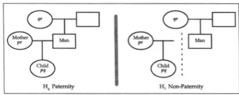
FIGURE 1.-The paternity problem posed as pedigrees.

tion for the simple trio situation above, although it will be assumed in the more general situations that follow. In the analysis the likelihoods X and Y could alterna- tively and equivalently have been defined with types of mother, man, and even mother’s contribution as part of the conditions rather than included in the hypothe- ses, as here. The present point of view lends itself more readily to generalization however, so serves better as a model for what follows.

Pedigrees: To recapitulate, the ordinary paternity

problem consists of comparing the two possible pat- terns of relatedness depicted in Figure 1. Some scien- tific evidence E, namely genetic types of the individuals involved, is determined. To assess the weight of the evidence E it is necessary and sufficient to evaluate the ratio X/ Y, where X = P(El paternity} and Y = P(E1 non- paternity} (EDWARDS 1972).

Once the paternity problem is cast in this abstract way, clearly many generalizations of it can be solved in the same way. Instead of the specific relationships Ho

and HI of Figure 1 , an arbitrary pair of “pedigrees,” each of which may be a family tree or trees, may be compared.

Two grandparents cme: The example shown in Figure 2

presents no new complications compared to the paternity case. One can write down by inspection that X = P(E1 Ho)

= 2p2qr2st *

‘/*

* where 2p2qr2st represents the proba-

bility that the three independent ancestors would have types as shown; and represent the probabilities of

p

and g filtering down to the child from the maternal and paternal sides, respectively. Similarly, Y =

f i E 1

HI} =

2p2qr2st. I/**

q.

where

q

is the chance that a random

sperm will have the allele g. Therefore X / Y =

One grandfinrent caw: The last case was simple in hav- ing only one possible origin for each of the child’s alleles. The general situation is more complicated be- cause there may be several combinations to consider.

n, ~ ~ n - ~ a ~ t y

FIGURE 2.-Putative grandparents tested instead of man.

FIGURE 3.-One putative grandparent tested instead of man.

Figure 3 is like Figure 2 but the putative grandfather was not tested. Computation of X therefore requires considering two ways to transmit a g allele from the paternal lineage: I/4 that the putative grandmother pas-

ses her g to the child, plus

q -

’/*

that the putative grand- father produces a g sperm, which subsequently passes to the child. Thus X / Y =

+

q / 2 ) / q .

Paternal ancestors: Rewriting the preceding results

as averages leads to an interesting observation. For the two grandparents case, note that X / Y = (I/2q

+

0 ) / 2 ;

for one grandparent, X / Y =

+

1 ) / 2 . The various terms in the numerators can be recognized as paternity indices corresponding to the types of the various al- leged grandparents, that is, interpret 0, and l as

the paternity indices when a qr person, an st person, or an untyped person, respectively, are evaluated as a possible father. Both as a preliminary to the general method and for its independent interest, it is worth- while exploring the rule suggested by these examples.

Paternal a n m t m rule: Suppose that a paternity problem involves no double relationships, and the genetic informa- tion available for a man consists of genetic types for some of his direct ancestors. Then his paternity index in each genetic system is the average of the paternity indices come- sponding to the types of his parents. Moreover, this rule can be iterated through previous generations.

To prove this rule, let

g,

h,

.

. .

be the various alleles at some locus. For an adult k define the vector of transmission

pobabi&?s T k (

-

), where T k ( g ) is the probability for person

k to pass allele

g

to an offspring given the types known for k and/or h‘s ancestors. If there is no information about the genetic types, T k ( g ) = I$ the frequency in nature of the allele

g.

If the genotype is known, then each Tk(g) is 0, or 1.

Using this notation the paternity index can be repre- sented asfollows. Let T ( * ) and T k ( * ) be the transmission probability vectors corresponding to mother and to an alleged father k . Let C be the set of genotypes consistent

with the phenotype of the child, so that

gh

E C means that the

gh

genotype gives the child’s phenotype. We can say

and Y = C,,,T(g)h. Then Lk = x k / Y is the paternity index for person k.

person k, andflk) to be the father. Under many circum- stances the condition

T k ( ' ) =

T f l k ) ( ' )

+

T m ( k ) (

.

)

0

L

holds, which we will refer to as condition S. For exam- ple, S is always true for a codominant system. For a multilocus system or one with silent alleles, like Rh, S still holds provided k's ancestors are unrelated, as does

Assume condition Sand assume that the mother and (1).

the man k are unrelated. Then

Lk =

x , / y =

[ 2 c r ( g ) T k ( h ) ] / Y

=[

ghE

c

C .(g) (Tflf(k)(h)

+

T m ( k ) ( h ) ) / 2 ] / Y

=

[.&

T(g)Tflk)(h)

+

gh€

c

c T ( g ) T m ( k ) ( h ) ] / ( e Y )

=[

(

&€

c

c T ( g ) T f l k i ( h ) ) / Y

+

(zc

T ( g ) T m ( k ) ( h ) ) / Y ] / 2 ,

2. e.,

Lk = [Lm(k)

+

Lflk)l/2,

(2)

which is the paternal ancestors rule.

Clearly the principle can be extended back through additional generations. For example, if the mother, m( m ( k ) ), of m ( k ) , is typed in her stead, then

Lm(m(k))

+

1

2

+ LAk)

Lk =

2

Here we have used that fact that, since flm( k ) ) is un-

The condition Sand therefore the paternal ancestors rule is rather general in its applicability. The mother may be typed or not; it works equally well in either case, so long as there exists a ~ ( g ) giving an adequate description of the mother's genetic contribution. It is not limited to single locus codominant systems, but is often also valid for systems of haplotypes such as the Rh system. However, it does not apply to a compound system defined by simultaneously considering the vari- ous combinations from two independent loci. There- fore, Formula 2 has to be applied one locus at a time. Thus, the paternal ancestors rule applies to HLA-AB only to the extent that recombination is ignored.

Avuncular indices: It is worth comparing the simple

situation of paternal ancestors just discussed with the more complex possibility that a sibling b of the alleged typed, Lflrn(k)) = 1.

father k is tested. That is, suppose we want to calculate the paternity index, Lk, of k by virtue of testing k's brother b. Equivalently, we can say that we are testing the brother b for uncle-hood. Consequently the term

avuncuZar index was proposed (MORRIS et al. 1988) for

the likelihood ratio Lk in such a case.2

Avuncular index rule: In a system for which genetic

types are available for child, alleged uncle band perhaps the mother, but not for b's brother k, and Lb is the paternity index for 6, the avuncular index Lk is

Lk = (Lb f 1 ) / 2 . (3)

In particular, in systems that exclude b from paternity his avuncular index is I/*, and in systems where the

paternity index is large, as a rule of thumb, the avuncu- lar index is about half as large.

To derive ( 3 ) , consider the genotypes of b's parents. Label the parents' allelles pr and qs (not necessarily distinct), and say b received alleles pq. Let T ~ ( * ) and T k ( * ) be conditional transmission probabilities vectors for b and k conditioned on the known phenotype of b. Now, Tb(g) = 4 p is a gl/2

+

4 q is a

&/2.

Each of p, q, r, or s has probability 1/4 to be transmitted by k, so

Tk(g) = -&4p 1 is

gl

+

4 q is

gl

+ fir

is

gl

+

4 s is g])

1 4

= -(27*(g)

+

270(g)),

where T O ( e ) : .rO(g) = g is the transmission vector of

nature, which is to say of a random person. That is,

T k ( ' ) = T b ( * )

+

2

T o ( * )

Since

L

= 1 , ( 3 ) can now be derived in the same way

as

(2).

Cases can arise where the above rules can be com- bined. For example, suppose that a man is tested and has a paternity index of L in some system. Since his avuncular index is ( L

+

1)/2, it follows by the paternal ancestors rule that the paternity index for his untested nephew is ( ( L

+

1 ) / 2

+

1)/2.

General problem: However, it is certainly not always

true that the transmission probabilities are an adequate substitute for genetic types. A situation wherein the method is inadequate is an untyped man with three children. Considering only his transmission probabil- ites seems to permit him to contribute a different allele to each one, but that is absurd. Hence at best the trans- mission probability approach is limited to analysis of single gametic events. Also, there does not appear to be a simple analogue of ( 3 ) corresponding to the case

2 In Latin, unfortunately, avunculus means maternal uncle (RON

GARNER, personal communication), but since there is no word in English derived from patrum (paternal uncle), avuncular index seems

of multiple typed siblings b, c,

. . .

of an alleged father k. This situation is discussed further below.

Consequently, to deal with arbitrary kinship prob- lems, a dynamic combinatorial approach is necessary. In the worst case it is necessary to explore a tree whose nodes correspond to all the different possible combina- tions of genotypes that all the people may have. The next section describes an algorithm, called the Kinship Program, that explores the tree.

THE KINSHIP PROGRAh4

The kernel of the program is a recursive subroutine that calculates Xor Y, i.e., calculates a likelihood P(El H),

where His a pedigree describing the hypothesized rela- tionships and E is the known phenotypes. The recursion iterates per person, from oldest to youngest. At each recursive level the program loops through the possible genotypes for the person, and the probabilities corre- sponding to each of these subcases are added.

Notation: To make the explanation more explicit,

further notation is needed.

People and relationships: Let the people be numbered 1, 2,

. . .

, k,

. . .

,

n, such that ancestors always precede descendants. In the following descriptions subscripts will always refer to people. Let mk denote the mother of person k, where mk = 0 if the mother is unspecified and is therefore to be taken as an unknown, untyped person; otherwise 0

<

mk

<

n. In particular, ml = 0. In a similar way& denotes the father of k. Sometimes the alternate notation m(k) or f(k) will be used to avoid double subscripts. A pair of ordered sets H = ( ( ml,

.

.

.)

,

(fi,

. .

.)) defines a pedigree.

Alleles and allelefrequencies: Let

p ,

q,

. . .

be names for the discrete alleles observed in any person, and

p,

q,

.

. .

be their respective frequencies of occurrence. All alleles never observed can be lumped together under the single name z, so that

p

+

q

+

-

-

+

z = 1.

Ordered genotypes: It will be useful to think of ordered genotypes rather than just genotypes, so for purposes of describing the algorithm

pq

will mean that

p

and q

are the maternally and paternally contributed alleles, respectively. As ordered genotypes,

pq

and

qp

each have frequency

p q

in the population.

Ordered genotype assignments: We will also need to con- sider assignments of ordered genotypes to the first k people, written G =

( C ; ,

G,

. . .

,

Gk), where each Gi =

gilti,

meaning that the ith person is considered to have inherited

gi

maternally and hi paternally. Let

e(

G) = k be the length of G. Let G

+

gh be

(C;,

G,

. . .

,

G,

gh), i.e., like Gwith the addition of an

e(

G) +lst person with the ordered genotype

gh.

Phenotypic data: For some people there are pheno- typic typing results. Write E = (El, l$,

.

.

.

,

E,) for the set of phenotypes, where Ek is the phenotype for person k. Phenotypes can be written pq or p or the special symbol

4

meaning that Ek is untyped. Since the relevant

fact about a phenotype is the genotypes that would manifest as that phenotype, we can think of pq as an abbreviation for

[pq,

q p } and t#~ as abbreviating [pp,

pq,

. . .

,

qp,

.

. .

,

zz).

That way it makes sense to say

p q E

pq or

pq

E

4.

If G, E E, for i = 1 ,

. . .

,

[(G), then we will say G is compatible with E.

Recursive algorithm: Now consider the probability

P(ElH, G) defined as follows. G is an assignment of ordered genotypes to the first

e(

G) = k people, and G is compatible with E. P(El H, G) means that given the pedigree H and assuming a genotype assignment G specified for the first k people, what is the probability to observe the evidence E?

If k = n, HE1 H,G] = 1.

If k

<

n, qElH,G)

= C g , h T m ( k + l ) ( g l G)T/(f(k+l)(hl G)P(EIH, G

+

(5)

where the sum is taken over all possible ordered geno- types gh E Ek+l, and T represents the transmission prob- abilities of the genes g and h from the mother and father of the k+lst person. Specifically, if

j>O

then

Tj(gl G) is 0 ,

'/*,

or 1 according as has 0,1, or 2 copies of the gene

g.

And

d g 1 G) =

g,

(6)

meaning that an unknown parent contributes

g

ac- cording to the frequency of g in the world.

Putting k = 0 , P(EIH,G} = P(ElH),

which gives either X or Y depending on whether H i s

Ho or HI. Then the likelihood ratio is X / Y.

Comments on the recursive formula: So the crux of

the algorithm is recursive evaluation of the Formula 5. Tree trimming: There are a few obvious steps to take to make the evaluation of (5) more efficient.

First, before recursion begins the phenotypes E are analyzed. Each person's phenotype Ek is written as a list of ordered genotypes. Then a backward pass is made through the relationships, from youngest person to old- est, and all ordered genotypes are removed that are incompatible with the relationships.

For example, if a child has phenotype pq and the mother is pr, then the list of possible child ordered genotypes is trimmed from

{pq, qp}

to just

{pq),

a poten- tial 50% reduction in evaluation steps. In the other direction, if the father of the same child is untyped, instead of considering all possible ordered genotypes for the father it will be enough to consider those with a q. If for example the possible alleles are

p ,

q, r, and z, the number of possibilities is thus reduced from 16 to seven. Notice that most of this reduction is recog- nized only because the genotypes are ordered (mater- nal contribution distinguished from paternal). Facilita- tion of tree-trimming is the main reason to deal with ordered genotypes.

539

up additional savings. Since the effort for each such pass is small and the benefit may be enormous, the trimming step is repeated until it has no further effect. The search reduction from this analysis can easily be

Second, during the recursive evaluation of ( 5 ) , the list of pairs gh, over which the summation occurs, is further limited by this rule: since there is no point in evaluating any flEl H, G

+

gh) that will have a coefficient of 0, only those gand h for which r

>

0 are considered.

Pedigree factoring: Sometimes the pedigree H consists of disjoint pieces, that is, the set of people can be parti- tioned into two or more sets with no interrelationships. This is normally the case under the alternative hypothe- sis, where typically the child, mother, and her relatives form one set, while the man and his relatives are pre- sumed to be an unrelated set.

The probability for the entire pedigree is then calcu- lated as the product of the probabilities for each of the independent pieces. If the number of combinations to inspect is u and w for the two pieces, then the total computation time will be only proportional to u

+

w

instead of to uw. Since u and w may be large numbers, the improvement seems well worthwhile. In practice, though, since there are two scenarios to evaluate and only one of them can be factored, the likely benefit is nearly 50%”useful, but not spectacular.

Symbolic evaluation: Evaluation of ( 5 ) consists only of adding and multiplying. Since each coefficient I- is ei- ther a constant or 1 ) or an allele frequency, each

f l E J H is a polynomial in the allele frequencies. This simple observation suggests doing the evaluation sym- bolically, adding and multiplying polynomials where the allele frequencies are letters, instead of arithmeti- cally. The symbolic operations of course take longer, but almost only by a constant f a ~ t o r . ~ Moreover, that constant is only about five, a small penalty thanks to the fact that the multiplications are all of a particularly simple kind: a polynomial times a monomial. No cross products arise. And the benefits are considerable; the symbolic program is much more interesting. The for- mula gives more information and has many uses. 1000-fold.

DISCUSSION

Examples: The examples in this section are all calcu-

lated by the Kinship Program. First are two typical prac- tical problems.

Inheritance problem: Arthur and Beatrice have dif-

ferent (dead) mothers. Arthur claims to be the sole child and heir of his dead father, but Beatrice believes she had the same father. She hopes to quantify the evidence of common alleles between herself and Arthur to establish her right to share the inheritance.

’Because the tree depth is not increased, only the time to visit each node. To be precise, the visit time is not strictly independent

of the size of the polynomial, but grows very slowly,

Suppose that Beatrice is right. Half-siblings figure to share no alleles in up to half of genetic systems (if the systems are highly polymorphic). In a genetic system where they have no similar alleles, the evidence is mod- estly against relationship. The likelihood ratio is

%.

In most of the remaining systems the sharing pattern will be

p,

ps and the likelihood ratio in favor of half-sibship is

+

1/(8p).

There is a subtle point to observe in applying these formulas. It is important to use a realistic estimate for the frequency

p,

not a conservative one as is the custom in paternity work. In a simple paternity case, paternity can eventually be proven by using sufficiently many markers even if the true evidentiary strength of each marker is squandered by using conservative allele fre- quency estimates. But accumulating the evidence in a case like this is like running up a down escalator. With every other system relentlessly chopping the likelihood ratio in half, the forward steps must be efficient lest there be no progress at all.

For example, suppose there are five systems with no shared alleles and five systems where an allele with fre- quency 0.05 is shared. Then the correct overall likeli- hood ratio is (1/2)5(1/2

+

5 / 2 ) 5 = ( 3 / 2 ) 5

=

8, substantial evidence for Beatrice’s point of view. But if the allele frequencies were “generously” estimated as 0.1, the overall likelihood ratio would be estimated as (‘/2)5(1/2

+

5/4)5 = (7/8)5

=

0.5, unfairly favoring Arthur.

Another half-sibling problem: Three men are either

brothers or half-brothers. They all have a common mother, but there are two fathers. The middle man, Milton, is a full brother either with the eldest, Ebenezer, or with the youngest, Yancy, but Ebenezer and Yancy have different fathers. DNA testing is done on Ebe- nezer, Milton, and Yancy to decide who Milton’s father was.

In three different loci, the sharing patterns for the three men are as follows:

Ebenezer Milton Yancy

Locus 1 _{p q}

_4T

_4s

Locus 2 _{p q}

_p.

S

Locus 3 _{p q qs Pr}

For the first locus the likelihood ratio is 1, since the pattern of genotypes is symmetrical about Milton.

At locus two, only Ebenezer and Milton share an al- lele. Superficially this suggests nominating them as the full-brother pair, but the likelihood ratio again is unity.

A combinatorial argument shows why: the

p

must be maternal, for otherwise the mother would have passed three different alleles to the three sons. Consequently, there is no evidence either way about fathers.

Locus three suggests that Milton is more likely to be Ebenezer’s brother, since they might share a paternal

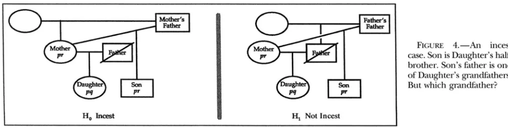
FIGURE 4.-An incest case. Son is Daughter’s half- brother. Son’s father is one of Daughter’s grandfathers. But which grandfather?

Ho Incest

9

Not Incest

I I

Kinship Program is 1

+

1/(2p

+

2q). If

p

and q are both rare, the evidence is quite strong.

An incest case: Figure 4 shows a complicated incest

case, the discussion of which will give a fair flavor of the workings of the program.

As illustrated by the diagram, Mother has two chil- dren. The father of the first child, Daughter, is the dead man called Father. The father of the second child, Son, is one or the other of Daughter’s grandfathers. The problem is to decide which grandfather. Genetic types are available just for Mother, Son, and Daughter.

The two scenarios to be compared are described to the program in the following notation:

Daughter

pq

: Mother pr

+

Father

The : separates the child’s name from her parents. The parents are separated by

+.

Lowercase letters, e.g., pq, optionally following a name are the phenotype of that person.

Son pr : Mother

+

MothersFather/FathersFather

The

/

separates two possibilities for a person. Son’s father is MothersFather under one scenario and Fa- thenFather under the other scenario.

Mother : ?

+

MothersFather

Mother’s parents are here defined to be an unknown person (?) and MothersFather.

Father : ?

+

FathersFather

Father’s parents are a different unknown person and FathersFather.

On initial analysis, there are four alleles to consider

( p ,

q, r, and z ) . Therefore there are 16 possible ordered genotypes for each of the untyped people, Father, MothersFather, and FathersFather, and two possibilities for each of Mother, Daughter, and Son. That amounts to -65,000 full length combinations for

G

to consider. Tree-trimming reduces this number to -8000, and in the end the number of evaluations of ( 5 ) is -900.

The variable z is undesirable because it has no mean- ing to the user. Besides, it is unnecessary. It can be eliminated using the relation z = 1

-

p

-

q

-

* * *

.

Elimination of z produces a great simplification, reduc- ing X from 20 terms to three and Y from 16 to two. It

is not clear why the disparity should be so great, nor even why the z-less form is the simpler, but typically it is so.

The final answer, after removing common factors from numerator and denominator, is (2

+

2p

+

2r)/

More avuncular indices: Armed with the general al-

gorithm, we can delve further into the situation where one or more siblings of the alleged father are tested. Suppose as before that mother is

p

and child is

pq.

Table 1 shows the paternity index for a variety of combi- nations of genotypes and numbers of siblings. Of course there are patterns to the formulae, but apparently there is no simple rule to combine multiple uncles and aunts in the way that there is for ancestors.

The next two examples explore published results. Twins: For twins to have the same genotype

pq

is evidence that they are monozygotic rather than dizy- gotic. Were the parents known to be pr and qs, the likelihood ratio would be exactly four. However, in the absence of typing the parents the possibility that one or both parents are homozygous reduces the likelihood ratio somewhat. The Kinship Program gives the formula 4/(1

+

p +

q

+

2pq) when the parents are not typed and the twins are heterozygous

pq.

In a system for which the twins are homozygous

qq,

the likelihood ratio is 4/ (1

+

q)2. The latter formula especially is not difficult to verify by hand and is also given in VOGEL and MOTULSKY (1986, p. 671). AKANE et al. (1991), on the other hand, gave different formulas for these situations.

The question of determination of zygosity of twins occurs frequently. Most often the reason is that one twin has leukemia and needs a bone marrow transplant. If the genetic match is perfect, then the recipient can be spared the risk of immunosuppressants. Since there is little theoretical benefit in typing the parents and neither leukemia nor twinship is particularly rare, the problem probably arises dozens of times per year.

Silent alleles and paternity cases: Among many possi-

ble enhancements to the program, a quite easy one was the inclusion of silent alleles. From the point of view of the kernel program this meant only adding more possible ordered genotypes corresponding to the ho- mozygous phenotypes:

p

is now (&by Po, op) where o is

the silent allele.

TABLE 1

Two singly U n i t e and one doubly infinite family of avuncular indices, where the paternal contribution is 9

~ ~ ~

No. of p q No. of 99 siblings of alleged father

siblings of

alleged father 0 1 2 3 4

0 1

_{- + -}

1 1 1 1 1 2 1 4

2q 2 2q

-+-

1 + q

-+-

2q 1 + 3q

-+-

2q 1 + 7q

1 (1/4g)(l

+

2q) 1 1/2 1 1 1 2 1 4

2 (1/4q)(1 + 3q - 2$(1

+

3p)) 1 1 1 2 1 4 1

-+-

-+-

-+-

-+-

2q 1

+

15q 2q l + q 2q 1

+

3q 2q 1

+

7q

- +

8

l + P + q + W 2q 1 + p + 3 q % + l + p + 7 q 2q

- +

l + p + 1 5 q % + 1 + p + 3 1 q

3 (1/4q)(l

+

5q - 12971

+

5P)) + 2 1 4 1 8 1 16

1

+

3p

+

3q

+

12pq 2g 1

+

3 p + 7q

5’

1

+

3 p + 15q

5’

1

+

3 p + 31q

2

9

’

1

+

3 p + 63q

As

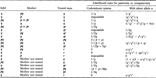
an application, Table

2

covers all patterns of

shared alleles, includes the case where the mother is not typed, and gives the formula both when silent alleles are considered possible and when not.

The last part of Table

2

covers the cases with an un- typed mother. BRENNER (1993) lists the motherless for- mulas for codominant systems, and the computer con- firms these simple formulas. CHAKRABORTY et al. (1994)

give formulas for the motherless case and silent alleles. In the first five of six cases the Kinship Program agrees. In the last case (the so-called “indirect exclusion,” a q

child and r man) they gave o being the frequency of silent alleles, not a plausible formula since it says that

the more rare is the silent allele, the more likely are father and child to have it. LUQUE and VALVERDE (1996)

have also made this point.

Limitations: The program as described is general but

does have some restrictions. The genetic systems must be codominant, or at most to have a silent allele. On the face of it this restriction could easily be removed: any autosomal genetic system can be set up by having a table containing genotype lists that correspond to each possible phenotype. Such a scheme would encom- pass Rh or MNSs, but not two loci of

HLA

unless recom- bination were ignored.

The present version presumes that all allele frequen-

TABLE 2

Likelihood ratios for various paternity situations

~~

Likelihood ratio for paternity vs. nonpaternity

Child Mother Tested man Codominant system With silent allele o

9 P9 9 1/q l/q’

9

P

9 impossible ( q ’ ” ’ ’ ) / q

P9

P

or@ 9 1/q ( q l / q l ‘ ) / q

9 9 9 1/q w q r - 0 3 / q ’ ( q

+

30))

P9

P

or@ 97 1/24

9

P

97 impossible 1/2q

9 P9 97 1/2q 1/2q‘

9 9 97 1/2q 1/2(q’ - d/q?

P9 P9 P9 1(/P

+

q )

Pn

Pa

9 1/(P + 4 ) ( q r / q r r ) / ( p

+

q )

P9 P9 97 1/(2P

+

2q)

9 P9 r 0 o / q ’ S

9 4 r 0 0/(q1Y

+

oqt”/q’)

9

P

r impossible 0

9 Mother not tested _{9 1/q (1}

₊

o ( l - o / q ” ) / q ) / q ”

P9 Mother not tested _{9 1/29 (qf/q‘‘)/2q}

9 Mother not tested _{97 1/2q (q’/q”)/2q}

P9 Mother not tested _P9

_{( P}

_{+ q)/4Pq}

P9 Mother not tested

_Pr

_1/44

4 Mother not tested r 0 o/ q”S

cies are from the same race. Allowing various races pres- ents no difficulty in principle; it would affect only (6).

Instead of a single symbol 0 to denote an untyped ances- tor, there need to be 0, 0’, O”, etc. for the various races. Then, additional symbols g‘,

g,

etc. would be introduced for allele frequencies of the extra races, where T0,(g) = g’, etc.

A few more restrictions are incidental to the kernel of the program and are only limitations of the Kinship input language through which the user describes the scenarios. For example, it might be more convenient if the program allowed comparison of more than two scenarios at once, although this is no limitation in prin- ciple because the scenarios can always be compared pairwise. The input description language necessitates that both scenarios include the same set of children. To describe the mono-/dizygotic twin scenarios therefore requires an artifice or “programming trick.”

Alleles must be discrete. With restriction fragment length polymorphism systems, where the reality is a col- lection of sizes none of which match exactly, the user has to decide which measurements represent identical alleles and which do not. In practice this is acceptable, but it would not be prohibitively hard to write a more general program that could deal with continuous allele measurements and measurement error, nor would such a program necessarily be very slow to run.

Conclusions: One motive for writing the Kinship

Program is that working out these problems by hand is very prone to error, as is shown by published errors.4 The program is interesting and useful because it gives clear and correct answers. The benefits of this include the following.

If the result is to be presented in an adversarial setting (in court), the formula can be given as justification for the calculation. Since the formula could perhaps be doubted as well as a number this justification at first sounds a bit circular, but in practice it is very helpful to be provided with this intermediate result. Typically, the formula can confidently be verified by hand even if deriving it de nouo would be very chancy.

The formulas can be instructive, surprising, and reveal- ing. The idea that realistic rather than conservative allele frequencies are necessary for half-sibling (and many other) cases is one example that is apparent from consid- eration of the formulas but previously escaped attention. Such rules as the simple general formulas for pater- nal ancestors and for uncles are more likely to be appar- ent given the relatively abstract point of view provided by symbolic likelihood ratios. The precise scope of these rules is hard to characterize. It depends in part on the complexity of the typing system. For example, consider

Unedited computer output will gladly be supplied on request for any problem discussed in this paper.

the allele transmission probabilities implied by knowl- edge of the parental types of an untyped alleged father. If the system is codominant, then also typing the alleged father’s uncle would change nothing, whereas for a more complicated system, such as AB0 or Rh, typing the uncle adds information. The complexity of the rela- tionships also bears on the applicability of the rules. On its face Equation 1 depends on the independence between maternal and paternal transmission probabili- ties; nonetheless in practice rule

(2)

holds even for some examples where mother and alleged father are related (while failing for similar examples). Also, there is interplay between the complexity of the genetic sys- tem and the degree to which the paternal ancestor or avuncular rule are tolerant of such relationships.

The static “transmission probability” approach con- trasts with the recursive algorithm (or “combinatorial approach”) embodied by the Kinship Program. The latter approach is necessary in general, but the princi- ple underlying the former, which is embodied in the rules (2) and ( 3 ) , applies in parts even to problems to which it does not provide a complete solution. Espe- cially (3) is conservative of formula complexity, in that it creates no new terms when applied to a ratio of poly- nomials. Thus the principle represents an effective re- duction that is one reason that the formula for even a large problem may well be simple.

Thanks to M. MCCINNISS and J. THOMAS for providing interesting examples. I am especially indebted to B. WEIR for invaluable advice and encouragement in preparing this paper.

LITERATURE CITED

AKANE, A., K. MATSLIBARA, H. SHIONO, M. YAMADA and Y . NUGOME, 1991 Diagnosis of twin zygosity by hypervariable RFLP markers.

Am. J. Med. Genet. 41: 96-98.

BRENNER, C., 1993 A note on paternity computation in cases lacking a mother. Transfusion 33: 51-54.

CHAKRABORW R., L. JIN and Y. ZHONG, 1994 Paternity evaluation in cases lacking a mother and nondetectable alleles. Int. J. Leg. Med. 107: 127-131.

CONWT, J., 1983 Serostatistische Abstammungsbegutachtung: ein Algorithmus fur Venuandtenfalle und das Daten- und Pro- grammsystem PAPS (dissertation). Gdrich & WeiersgLuser, Mar-

EDWARDS, A. W. F., 1972 Likelihood, An Account of thestatistical Concept

burg Germany.

of Likelihood and Its Application to Scientijic Infmence. Cambridge University Press, Cambridge.

IHM, P., and K. HLIMMEI., 1975 A method to calculate the plausibility

of paternity using blood groups results of any relatives. Z. Immun- iatsforsch. Exper. Klin. Immunol. 149: 405-416.

LUQUE, J. A,, and J. L. VAVERDE, 1996 Paternity evaluation in cases lacking a mother and non-detectable alleles (letter). Int. J. Leg.

Med. 108: 229.

MORRIS, J. W., R. A. GARBER, J. D’AUTREMONT and C. H. BRENNER, 1988 The avuncular index and the incest index. Adv. Forensic

VOGEL F., and A. G. MOTULSKY, 1986 Human Genetics: Problemc L+

Haemogenet. 2 607-611.

Approaches, Ed. 2. Springer-Verlag, Berlin.

WALKER, R. A,, 1983 Inclusion Probabilities i n P a l a i t y Testing, h e r . Assoc. of Blood Banks, Arlington, VA.