Page 1 of 27
Automatic Bedrock and Ice Layer
Boundaries Estimation in Radar Imagery
Based on Level Set Approach
Maryam Rahnemoonfar1, Geoffrey C. Fox2, Masoud Yari3
1 Department of Computing Sciences, Texas A&M University-Corpus Christi, TX 78412 2 School of Informatics and Computing, Indiana University, Bloomington
3 Department of Engineering, Texas A&M University-Corpus Christi, TX 78412
Abstract
Accelerated loss of ice from Greenland and Antarctica has been observed in recent
decades. The melting of polar ice sheets and mountain glaciers has a considerable influence on
sea level rise in a changing climate. Ice thickness is a key factor in making predictions about the
future of massive ice reservoirs. The ice thickness can be estimated by calculating the exact
location of the ice surface and hidden bedrock beneath the ice in radar imagery. Identifying ice
surface and bedrock locations is typically performed manually which is a very time consuming
procedure. Here we propose an approach which automatically detects ice surface and bedrock
boundaries using distance regularized level set evolution. In this approach the complex topology
of ice and bedrock boundary layers can be detected simultaneously by evolving an initial curve
in radar imagery. Using a distance regularized term, the regularity of the level set function is
intrinsically maintained that solves the reinitialization issues arising from conventional level set
approaches. The results are evaluated on a large dataset of airborne radar imagery collected
during IceBridge mission over Antarctica and Greenland and show promising results in respect
Page 2 of 27
1. Introduction
Page 3 of 27
[image:3.612.76.528.75.229.2]
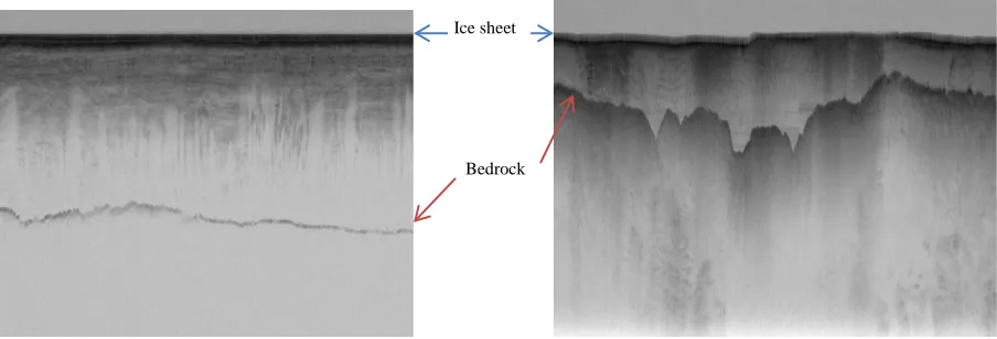
Figure 1: Ice sheet and bedrock depicted in radar echogram gathered by the Multichannel Coherent Radar Depth Sounder
The large variability of bedrocks shape along with speckle noise inherits from the coherent nature of SAR images, make the identification and interpretation of bedrocks quite difficult. Usually human experts mark ice sheet layer and bedrock by hand for further processing. Manual layer identification is very time consuming and is not practical for regular, long-term ice-sheet monitoring. The development of automated techniques is thus fundamental for proper data management.
This paper proposes a novel level set approach to automatically identify ice layer and bedrock in a large dataset of radar imagery. In this approach the image will be segmented by an initial curve into two parts: inside the curve (negative interior) and outside the curve (positive exterior). At the next step, each point on the curve will move at variable speeds depending on their distance from the center of the curve. Nearer points move faster while further points move at lower speeds. In the case of having a feature in the image, shrinking (expanding) curve will stop at the boundary of the shape. This process will continue until all boundaries are detected. In conventional level set formulation, the level set function typically develops irregularities during its evolution
Page 4 of 27
and needs re-initialization to periodically replace the degraded level-set function. Here we used a variational level set function in which the regularity of level set function is maintained intrinsically.
After this introduction, the related works will be discussed in section 2. The details of the proposed method will be discussed in section 3. Experimental results will be discussed in section 4. Finally conclusions are drawn in section 5.
2. Related works
Page 5 of 27
Several works in the literature use graphical models to detect land mine [4] or ice layers [5] [6] in radar echograms. Frigui et al [4] proposed a system for land mine detection using ground-penetrating radar. Their proposed system includes a hidden Markov model based detector, a corrective training component, and an incremental update of the background model. Crandall et al [5] used probabilistic graphical models for detecting ice layer boundary in echogram images. Their model incorporates several types of evidence and constraints including that layer boundaries should lie along areas of high image contrast and that layer boundaries should be continuous and not intersect. The extension of this work was presented in [6] where they used Markov-Chain Monte Carlo to sample from the joint distribution over all possible layers conditioned on an image. Gibbs sampling instead of dynamic programming based solver was used for performing inference. The problem with using graphical models is that it needs a lot of training samples (around half of the actual dataset) which are ground-truth images labeled manually by human. Given the fact that manual ice layer detection is a very time consuming and expensive task, the last three methods are not practical for large dataset.
Page 6 of 27
incapability of maintaining the topology of evolving curve. This difficulty does not arise in the level set model as it embeds the evolving curve into a higher dimensional surface. Mitchell et al [12] used level set technique for estimating bedrock and surface layers. However for each single image the user needs to re-initialize the curve manually and as a result the method is quite slow and was applied only to a small dataset. In this paper, the regularity of level set is intrinsically maintained using a distance regularization term. Therefore it does not need any manual re-initialization and was automatically applied on a large dataset.
3. Methodology
Here we propose to use level sets technique to precisely detect ice layer and bedrock boundary. The level set method (LSM) is essentially a successor to the active counter method. Active contour method (ACM), also known as Snake Model, was first introduced by Kass et al [15]. The ACM is designed to detect interfaces and boundaries by a set of parametrized curves (contours) that march successively toward the desired object until the desired interfaces are captured. We present the parametrized curves as
( , ) ( ( , ), ( , )) , [0,1], [0, )
C s t = x s t y s t s∈ t∈ ∞ (1)
Page 7 of 27
Generally speaking, the curve C s t( , ) moves and eventually captures the interface of the desired object according to the following differential equation
C FN t ∂
=
∂ (2)
where F is the velocity function for the moving curve C and N determines the direction of the motion. Here N is the normal vector to the curve C.
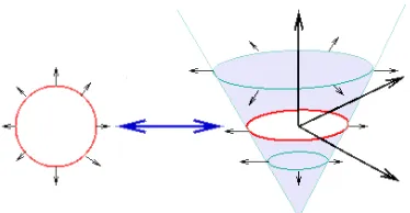
[image:7.612.229.416.545.642.2]The ACM is an efficient tool in image and video segmentation, but it suffers from certain serious issues. As mentioned before, the main disadvantage of the ACM is that it is incapable to maintain the topology of the evolving curve; therefore, it can introduce misleading complexities in the process. To overcome the disadvantages that the snakes model presents, the level set method (LSM) was proposed by Osher and Sethian [16]. Rather than following the interface itself as in ACM, the level set method takes the original curve and builds it into a surface. In other words, the LSM takes the problem to one degree higher in spatial dimension and considers the curve C s t( , ) as the zero-level of a surface z=ϕ( , , )x y t at any given time t. The function
ϕ
is called the level set function (LSF).Page 8 of 27
suppose the curve C s t( , ) is the interface of an open region 2
t
Ω ⊂ . We embed the curve C s t( , ) in the surface z=ϕ( , , )x y t in a way that the curve C s t( , ) will be the zero level set while LSF,
ϕ
, takes negative values inside C and positive values outside of it. That is( )
x t, 0 for x t,ϕ = ∈∂Ω (3)
and
( )
( )
, 0 , 0 t tx t for x
x t for x
ϕ ϕ
< ∈ > ∉
Ω ,
Ω . (4)
In this setting, the LSF,
ϕ
, is the solution of the following dynamical system(x t, ) [0, ]
t
ϕ
ϕ ∈
∂ =−∂ Ω×
∂ ∂ ∞
F
(5)
with a typical initial condition. Conventionally in image segmentation approaches the LSF functional F is defined as the sum of the edge force and the area force:
edge area =E +E
F (6)
where
( )
( )
edge ϕ =λ
∫
Ωgδ ϕ ∇ϕ dxE (7)
( )
( )
area ϕ =α
∫
ΩgH −ϕ dxE (8)
Page 9 of 27
2
1 1 g
Gσ I =
+ ∇ ∗ (9)
where I is the image intensity and Gσ is a Gaussian Kernel with a standard deviation
σ .
The edge term, Eedge computes the line integral along the zero level contour of
ϕ
;that is, 1
0g C s( ( )) |C s'( ) |ds
∫
, where the curve C=C s( ) :[0,1]→ Ω is the zero-level contourand s is the curve length. This term will be minimized when C is positioned on the boundary of the desired object. The area term, Earea, is basically calculated as a weighted area of the region inside the zero level contour. It accelerates the motion of the zero-level contours toward the desired object.
Therefore, to minimize the energy functionalF , it is necessary to solve the following PDE system:
0
( ) div ( ) [0, )
| |
( , 0) (
( )
)
, x t
t g g
x x
ϕ
λδ ϕ α δ
ϕ
ϕ ϕ
ϕ ϕ
∇ + ∈Ω× ∞
∇
= ∂ =
∂ (10)
For this system we consider the Neumann boundary condition on Ω, which signifies that there is no external force outside the image area. To carry out a numerical process to solve this PDE system, the spatial derivatives are discretized using the upwind scheme. The use of the central difference scheme will result in instability in the numerical procedure. The numerical procedure also involves the assumption that
Page 10 of 27
care, known as re-initialization, must be taken to avoid the error accumulation. The reinitialization procedure involves solving the following PDE system for ψ in each step
( )(1 | |) sign
t
ψ ϕ ψ
∂
= − ∇
∂ (11)
This severely slows down the computation. To overcome this difficulty we use the distance regularization method proposed in [17] [18]. In DSLR method, the LSF functional F is defined as
edge area p =E +E +E
F (12)
where Ep represents the distance regularization term defined by
( )
Ω
| | p ϕ =
∫
p ∇ϕ dxE (13)
with a potential function p and a constant µ>0. As suggested in [18] , we use a double-well function for the potential function p defined by
2
2
(1 cos(2 ) ( )
( 1) ) / 4
1 / 2 1 s s p s s s π π − ≤ − ≥ =
(14)
We have
d v(i ) p D µ ϕ ϕ ∂ − ∂ = ∇ E (15)
where the diffusion coefficient D=D( )ϕ is given by
' (| | . |
( ) )
|
Dϕ p ϕ
ϕ ∇ =
Page 11 of 27
We note that p has two minimum points at s=0 and s=1. It is also twice differentiable with the following properties
0
'( ) '( ) '( )
| | 1 for 0 , and lim lim 1.
s s
p s p s p s
s
s < > → s = →∞ s = (16)
Given the above properties, one can easily see that ' (| |) | | . | | p ϕ µ µ ϕ ∇ ≤
∇ (17)
Therefore the diffusion coefficient in (17) will be bounded. Now the new energy functional F can be minimized by solving the following gradient flow:
0
d
( ) div ( ) ) [0, )
| | ( iv , 0 ( ) ) ( , ( ) g g x D x x t t ϕ
λδ ϕ α δ ϕ µ ϕ
ϕ ϕ
ϕ
ϕ
∇
+ + ∇ ∈Ω× ∞
∇ = ∂ =
∂ (18)
Thanks to the distance regularization term, the central difference scheme can be used to
discretize spatial derivatives, which leads to a stable numerical procedure without need of
re-initialization [18].
It also must be noted that, in practice, the functions δ and H are approximated by the
smooth functionsδε and Hε defined by (see [19] and [20])
( )
21 1 cos ,Page 12 of 27
( )
1 1
1 sin ,
2
1 | | ,
0 | | ;
x x x H x x x ε π ε
ε π ε
ε ε + + ≤ = >
< −
(20)
for ε >0. εis often considered to be 3/2.
As the boundary condition, we consider the Neumann boundary conditions. For the initial
condition, we will consider a simple step function defined by
0 0 0 0 0 , ; / c x c x
ϕ = − ∈Ω
∈Ω Ω
(21)
where c0 >0 is a constant, and Ω0 is a region inside the image region Ω.
4. Experimental results
Page 13 of 27
need any training dataset and our method is not affected by inaccurate ground-truth. Moreover annotating data by human is quite time consuming and because our method does not need any training and is independent of ground-truthing, it is quite fast. We used the same iteration number of 800 for all of the images.
Page 14 of 27
(a) (b)
(c) (d)
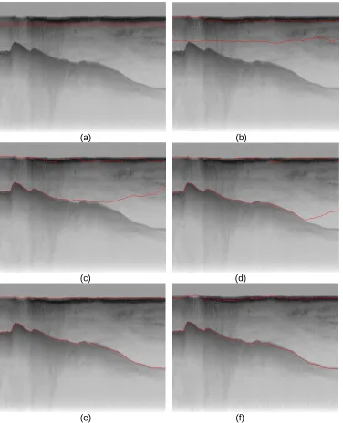
[image:14.612.121.497.70.534.2]
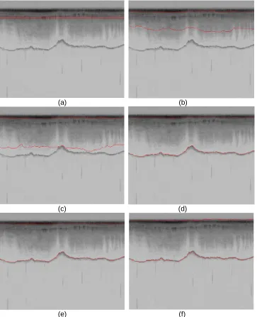
(e) (f)
Figure 3: contour evolution throughout processing. a) Initial curve, (b)-(e) contour adaptation to bedrock and ice layer after 200,400,600,800, correspondingly, (f) ground-truth image
Page 15 of 27
images. As it can be seen in Figure 4e the perfect shapes of bedrock and ice layers are maintained and extra iterations will not make the situation worse. Comparing our results (Figure 4e) with the ground-truth (Figure 4f), we find our results are more smooth and accurate than ground-truth.
(a) (b)
(c) (d)
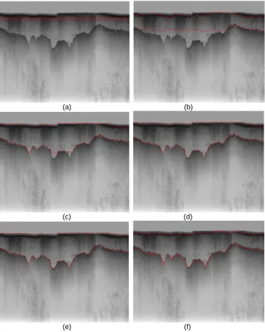
[image:15.612.121.493.201.667.2]
(e) (f)
Page 16 of 27
Figure 5 demonstrates another example for ice and bedrock layers identification. Here the bedrock is smoother but the image contains more noise especially in the middle layer between ice and bedrock. Here again with the same initial curve and the same number of iterations we got very accurate results comparing to the ground-truth.
(a) (b)
(c) (d)
[image:16.612.127.490.188.635.2]
(e) (f)
Page 17 of 27
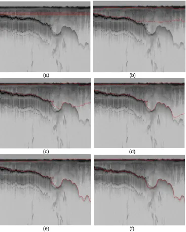
Figure 6 is yet another example with more complicated shape of bedrock and with high level of noise in the entire image. Here it takes the entire 800 iterations for the level set solution to converge but it shows a very satisfactory results comparing to the ground-truth.
(a) (b)
(c) (d)
[image:17.612.124.491.187.646.2]
(e) (f)
Page 18 of 27
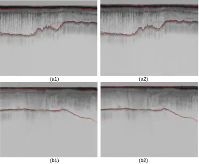
Figure 7 shows some of the representative results for the ice and bedrock layer identification for various shapes of bedrock from a very smooth bedrock to a rough and very oscillating bedrock with different levels of noise. In all of the examples, the results with the automatic level-set approach (the left column) is as accurate as ground-truth (the right column). However in the last two rows (f1 and g1) due to high level of fluctuations in the bedrock, still after 800 iterations it could not detect all parts of the bedrock. However the results are very close to ground-truth and more iteration will create more accurate results. In this study we used the constant iterations of 800 for all of the images in the dataset.
(a1) (a2)
Page 19 of 27
(c1) (c2)
(d1) (d2)
Page 20 of 27
(f1) (f2)
(g1) (g2)
Figure7: Bedrock and ice layer detection by proposed method, left column: the result of the proposed level set approach, Right column: ground-truth
5. Evaluation
Page 21 of 27
Actual Class (Observation)
Predicted Class (Expectation)
TP (True Positive)
Correct result
FP (False Positive)
Unexpected result FN
(False Negative) Missing result
TN (True Negative) Correct absence
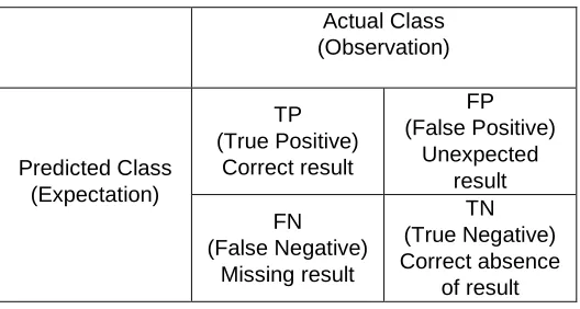
[image:21.612.175.439.81.222.2]of result Table 1: Confusion Matrix
In the confusion matrix, TP is true positive or correct result, FP is false positive or unexpected result, FN is false negative or missing results, and TN is true negative or correct absence of results. From the confusion matrix recall (R) and precision (P) are calculated as follow:
𝑅𝑅 = 𝑇𝑇𝑇𝑇𝑇𝑇𝑇𝑇+𝐹𝐹𝐹𝐹
(1)
𝑇𝑇= 𝑇𝑇𝑇𝑇𝑇𝑇𝑇𝑇+𝐹𝐹𝑇𝑇
(2)
Precision measures the exactness of a classifier while recall measures the completeness or sensitivity of a classifier. Precision and recall can be combined to produce a single metric known asF-measure, which is the weighted harmonic mean of precision and recall. The F-measure defined as:
𝐹𝐹 = 1
𝛼𝛼1𝑝𝑝+ (1− 𝛼𝛼) 1𝑅𝑅 =
(𝛽𝛽2+ 1)𝑇𝑇𝑅𝑅 𝛽𝛽2𝑇𝑇+𝑅𝑅
Page 22 of 27
captures the precision and recall tradeoff. The F-measure is valued between 0 and 1, where larger values are more desirable. In this paper we used balanced F-measure, i.e. with 𝛽𝛽 = 1 .
Page 23 of 27
Figure 8: F-measure, precision and recall for all 323 images
0 0.1 0.2 0.3 0.4 0.5 0.6 0.7 0.8 0.91
1 16 31 46 61 76 91 106
12 1 13 6 15 1 16 6 18 1 19 6 21 1 22 6 24 1 25 6 27 1 28 6 30 1 31 6 F-me as ure Image-ID 0 0.1 0.2 0.3 0.4 0.5 0.6 0.7 0.8 0.9 1
1 16 31 46 61 76 91 106
12 1 13 6 15 1 16 6 18 1 19 6 21 1 22 6 24 1 25 6 27 1 28 6 30 1 31 6 Pr ec isio n Image-ID 0 0.1 0.2 0.3 0.4 0.5 0.6 0.7 0.8 0.91
1 16 31 46 61 76 91
Page 24 of 27
Precision Recall F-measure
[image:24.612.150.465.86.152.2]Our approach 74% 77% 75%
Table 2: Average Precision, Recall and F-measure of our approach for the entire dataset
(a)
(b) (c)
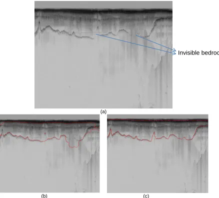
Figure 9: our approach is not able to detect the invsible parts of bedrock, a) original image, b) the icelayer and bedrock detected by our approach, c) ground-truth
[image:24.612.117.555.215.611.2]Page 25 of 27
6. Conclusion
We presented an automatic approach to estimate bedrock and ice layers in multichannel coherent radar imagery. In this approach the complex topology of ice and bedrock boundary layers were detected by evolving an initial curve in radar imagery. The results were evaluated on a large dataset of airborne radar imagery collected during IceBridge mission over Antarctica and Greenland and show promising results in respect to hand-labeled ground truth. We reached the high accuracy of 75% for the entire dataset using a fully automatic technique. Some images present faint or invisible bedrock layers and are nearly impossible to automatically detect them with 100% accuracy. For those images it is better to first separate them from the images that have visible bedrock layer. Then for each dataset we will have different parameters for level set algorithm. In future we are planning to extend this work by improving the quality of the image in fain and invisible areas in bedrock prior to applying level set algorithm.
7. References
1.
Allen, C., et al.,
Antarctic ice depthsounding radar instrumentation for the
NASA DC-8.
Aerospace and Electronic Systems Magazine, IEEE, 2012.
27
(3): p. 4-20.
2.
Freeman, G.J., A.C. Bovik, and J.W. Holt.
Automated detection of near
surface Martian ice layers in orbital radar data
. in
Image Analysis &
Interpretation (SSIAI), 2010 IEEE Southwest Symposium on
. 2010. IEEE.
3.
Ferro, A. and L. Bruzzone.
A novel approach to the automatic detection of
subsurface features in planetary radar sounder signals
. in
Geoscience and
Remote Sensing Symposium (IGARSS), 2011 IEEE International
. 2011.
IEEE.
4.
Frigui, H., K. Ho, and P. Gader,
Real-time landmine detection with
ground-penetrating radar using discriminative and adaptive hidden Markov models.
Page 26 of 27
5.
Crandall, D.J., G.C. Fox, and J.D. Paden,
Layer-finding in Radar Echograms
using Probabilistic Graphical Models.
6.
Lee, S.-R., et al.
Estimating bedrock and surface layer boundaries and
confidence intervals in ice sheet radar imagery using MCMC
. in
Image
Processing (ICIP), 2014 IEEE International Conference on
. 2014. IEEE.
7.
Gifford, C.M., et al.,
Automated polar ice thickness estimation from radar
imagery.
Image Processing, IEEE Transactions on, 2010.
19
(9): p.
2456-2469.
8.
Ilisei, A.-M., A. Ferro, and L. Bruzzone.
A technique for the automatic
estimation of ice thickness and bedrock properties from radar sounder data
acquired at Antarctica
. in
Geoscience and Remote Sensing Symposium
(IGARSS), 2012 IEEE International
. 2012. IEEE.
9.
Karlsson, N.B., et al.,
Tracing the depth of the Holocene ice in North
Greenland from radio-echo sounding data.
Annals of Glaciology, 2013.
54
(64): p. 44-50.
10.
Fahnestock, M., et al.,
Internal layer tracing and age
‐
depth
‐
accumulation
relationships for the northern Greenland ice sheet.
Journal of Geophysical
Research: Atmospheres (1984–2012), 2001.
106
(D24): p. 33789-33797.
11.
Sime, L.C., R.C. Hindmarsh, and H. Corr,
Instruments and methods
automated processing to derive dip angles of englacial radar reflectors in
ice sheets.
Journal of Glaciology, 2011.
57
(202): p. 260-266.
12.
Mitchell, J.E., et al.
A semi-automatic approach for estimating bedrock and
surface layers from multichannel coherent radar depth sounder imagery
. in
SPIE Remote Sensing
. 2013. International Society for Optics and Photonics.
13.
Mitchell, J.E., et al.
A semi-automatic approach for estimating near surface
internal layers from snow radar imagery
. in
IGARSS
. 2013.
14.
Chan, T.F. and L. Vese,
Active contours without edges.
Image processing,
IEEE transactions on, 2001.
10
(2): p. 266-277.
15.
Kass, M., A. Witkin, and D. Terzopoulos,
Snakes: Active contour models.
International journal of computer vision, 1988.
1
(4): p. 321-331.
16.
Osher, S. and J.A. Sethian,
Fronts propagating with curvature-dependent
speed: algorithms based on Hamilton-Jacobi formulations.
Journal of
computational physics, 1988.
79
(1): p. 12-49.
17.
Li, C., et al.
Level set evolution without re-initialization: a new variational
formulation
. in
Computer Vision and Pattern Recognition, 2005. CVPR
2005. IEEE Computer Society Conference on
. 2005. IEEE.
Page 27 of 27