Finding and counting tree-like subgraphs using
MapReduce
Zhao Zhao, Langshi Chen, Mihai Avram, Meng Li, Guanying Wang, Ali Butt, Maleq Khan,
Madhav Marathe, Judy Qiu, Anil Vullikanti
Abstract—Several variants of the subgraph isomorphism problem, e.g., finding, counting and estimating frequencies of subgraphs in networks arise in a number of real world applications, such as genetic network analysis in bioinformatics, web analysis, disease diffusion prediction and social network analysis. These problems are computationally challenging to scale to very large networks with millions of nodes. In this paper, we present SAHAD, a MapReduce based algorithm for detecting and counting trees of bounded size using the elegant color coding technique, developed by N. Alon, R. Yuster and U. Zwick, Journal of the ACM (JACM) 1995. SAHADis a randomized algorithm, and we show rigorous bounds on the approximation quality and the performance. We implement SAHADon two different frameworks: the standard Hadoop model and Harp, which is more of a high performance computing environment, and evaluate its performance on a variety of synthetic and real networks. SAHADscales to very large networks comprising of107−108 nodes and108−109edges and tree-like (acyclic) templates with up to 12 nodes. Further, we extend our results by implementing our algorithm using the Harp framework. The new implementation gives two orders of magnitude improvement in performance over the standard Hadoop implementation and achieves comparable or even better performance than start-of-the-art MPI solution.
Index Terms—subgraph isomorphism, graph partitioning, MapReduce, Hadoop, Harp
F
1
I
NTRODUCTIONG
IVENtwo graphsGandH, the subgraph isomorphism problem asks ifH is isomorphic to a subgraph of G. The counting problem associated with this seeks to count the number of copies ofH in G. These and other variants are fundamental problems in Network Science and have a wide range of applications in areas such as bioinformatics, social networks, semantic web, transportation and public health. Analysts in these areas tend to search for meaningful patterns in networked data; and these patterns are often spe-cific subgraphs such as trees. Three different variants of sub-graph analysis problems have been studied extensively. The first version involves counting specific subgraphs, which has applications in bioinformatics [4], [16]. The second involves finding the most frequent subgraphs either in a single network or in a family of networks—this has been used in finding patterns in bioinformatics (e.g., [20]), recom-mendation networks [22], chemical structure analysis [30], and detecting memory leaks [25]. The third involves find-ing subgraphs which are either over-represented or under-represented, compared to random networks with similar• Zhao Zhao, Ali Butt, Madhav Marathe and Anil Vullikanti are with the
Network Dynamics and Simulation Science Laboratory, Biocomplexity Institute & Department of Computer Science, Virginia Tech, VA, 24061. E-mail: [email protected], [email protected], [email protected], [email protected]
• Maleq Khan is with the Department of Electrical Engineering and
Com-puter Science, Texas A&M University-Kingsville. E-mail: [email protected]
• Langshi Chen, Meng Li, and Mihai Avram are with the Computer Science
Department, Indiana University.
Email: [email protected], [email protected], [email protected]
• Judy Qiu is with the Intelligent Systems Engineering Department,
Indi-ana University. Email: [email protected]
• Guanying Wang is working with Google Inc.
Email: [email protected]
properties—such subgraphs are referred to as “motifs”. Milo et al. [26] identify motifs in many networks, such as protein-protein interaction (PPI) networks, ecosystem food webs and neuronal connectivity networks. Subgraph counts have also been used in characterizing networks [28].
The Subgraph Isomorphism problem and its variants is well known to be computationally challenging. In general the decision version of the problem is NP-hard, and the counting problem is #P-hard. Extensive work has been done in theoretical computer science on this problem; we refer the reader to the recent papers by [10], [12], [24] for an extensive discussion on the decision and counting complexity of the problem and tractable results for various parameterized versions of the problem.
The primary focus of this paper is on the three men-tioned variants of the subgraph isomorphism problem when
k, the number of nodes in the templateH, is fixed. Letting
n be the number of nodes inG, one can immediately get simple algorithms with running time O(nk) to find and
count the number of copies of templateH in G. Note that in this paper we focus on non-induced subgraph matching. When the template is a tree or has a bounded treewidth,
Alon et al. [4] present an elegant randomized
approxima-tion algorithm with running timeO(k|E|2keklog (1/δ)ε12),
whereεandδare error and confidence parameters, respec-tively, based on the color coding technique. There result was significantly improved by Koutis and Williams [19] who gave an algorithm with running time ofO(2k|E|).
IEEE TRANSACTIONS ON MULTI-SCALE COMPUTING SYSTEMS 2 pruning and exploration techniques, e.g., [15], [20], [40].
Other approaches in relational databases and data mining involve queries for specifically labeled subgraphs, and have combined relational database techniques with careful depth-first exploration, e.g., [8], [31], [32].
Most of these approaches are sequential, and generally scale to modest size graphs G and templates H. Paral-lelism is necessary to scale to much larger networks and templates. In general, these approaches are hard to par-allelize as it is difficult to decompose the task into inde-pendent subtasks. Furthermore, it is not clear if candidate generation approaches [15], [20], [40] can be parallelized and scaled to large graphs and computing clusters. Two recent approaches for parallel algorithms, related to this work, are [8], [41]. The approach of Br ¨ocheler et al. [8] requires a complex preprocessing and enumeration process, which has high end-to-end time, while the approach of [41] involves an MPI-based implementation with a very high communication overhead for larger templates. Two other papers [27], [36] develop MapReduce based algorithms for approximately counting the number of triangles with a work complexity bound ofO(|E|). The development of par-allel algorithms for subgraph analysis with rigorous poly-nomial work complexity, which are implementable on het-erogeneous computing resources remains an open problem. Due to the complexity of enumerating subgraphs, people propose to compute some metrics of the subgraph which is anti-monotone to the subgraph size. The algorithm reported in [3] is capable of computing subgraph support on large networks with up to 1 Billion edges. However, it requires each machine to have a copy of the graph in memory which limits its scalability to larger graphs. Additionally, computing support requires much less computational effort than counting subgraphs. Another recent work also employs MapReduce to match subgraphs [35] which scales to net-works with up to 300 million edges.
Other approaches studied in the context of data mining and databases, e.g., [8], [31], [32], are capable of processing large networks, but are usually slow due to limitations of database techniques for processing networks.
Our contributions. In this paper, we present SAHAD, a
new algorithm for Subgraph Analysis using Hadoop, with rigorously provable polynomial work complexity for several variants of the subgraph isomorphism problem whenH is a tree. SAHAD scales to very large graphs, and because of the Hadoop implementation, runs flexibly on a variety of computing resources, including Amazon EC2 cloud. We also adapt SAHAD in the Harp [29] framework to utilize its advanced MPI-like collective communication. It scales to graphs with up to1.2billion edges.
Our specific contributions are discussed below.
1. SAHAD is the first MapReduce-based algorithm for finding and counting labeled trees in very large networks. The only prior Hadoop based approaches have been on triangles [27], [36], [37] on very large networks, or more general subgraphs on relatively small networks [23]. Our main technical contribution is the development of a Hadoop version of the color coding algorithm of Alon et al. [4], [5], which is a (sequential) randomized approximation algo-rithm for subgraph counting. It is a randomized approxima-tion algorithm that for anyε, δ, gives a(1±ε)approximation
to the number of embeddings with probability at least 1−2δ. We prove that the work complexity of SAHAD is
O(k|EG|22keklog (1/δ)ε12), which is more than the running
time of the sequential algorithm of [4] by just a factor of2k.
2. We demonstrate our results on instances generated using the Erd ¨os-Renyi random graph model, the Chung-Lu random graph model and on synthetic social contact graphs for Miami city and Chicago city (with 52.7 and 268.9 million edges, respectively), constructed using the methodology of [7]. We study the performance of counting unlabeled/labeled templates with up to 12 nodes. The total running times for templates with 12 nodes on Miami and Chicago networks are 15 and 35 minutes, respectively; note that these are thetotal end-to-endtimes, and do not require any additional pre-processing (unlike, e.g. [8]).
3.We discuss how our basic algorithms for counting sub-graphs can be extended to compute supervised motifs and graphlet frequency distributions. They can also be extended to count labeled subgraphs.
4. SAHAD runs easily on heterogeneous computing re-sources, e.g., it scales well when we request up to16nodes on a medium size cluster with 32 cores per node. Our Hadoop based implementation is also amenable to running on public clouds, e.g., Amazon EC2 [6]. Except for a 10-node template which produces extremely large amount of data so as to incur the I/O bottleneck on the virtual disk of EC2. It is worth noting here that the performance of SAHADon EC2 is almost the same as on the local cluster. This would enable researchers to perform useful queries even if they do not have access to large resources, such as those required to run previously proposed querying infrastructures. We believe this aspect is unique to SAHAD and lowers the
barrier-to-entry for scientific researchers to utilize advanced computing resources.
5.We study the performance improvement in extensions of the standard Hadoop framework. The enhanced algo-rithm is called EN-SAHAD. First, we consider techniques to explicitly control the sorting and inter partition communica-tions in Hadoop. We find that reducing the sorting step by pre-allocating can improve the performance by about 20%, but improved partitioning does not seem to help.
6.Finally, we implement SAHAD within the Harp [29] framework – the new algorithm is called HARPSAHAD+. HARPSAHAD+ yields an order of magnitude improve-ment in performance, as a result of its flexibility in task scheduling, data flow control and in memory cache. We are therefore able to scale to networks with up to billions of edges using the HARPSAHAD+ and obtain a comparable performance when compared to a state-of-the-art MPI/C++ implementation.
Organization. Section 3 introduces the background for the
while section 8 discusses experiment results of SAHAD, EN
-SAHAD and HARPSAHAD+. Finally, Section 9 concludes the paper.
Extension from conference version.The SAHADalgorithm
appeared in [42]. The results on EN-SAHADand HARP SA-HAD+ are new additions. Since the publication of [42], there has been more work done on parallelizing the color coding technique, e.g., [33], [34]. However, none of these have been based on MapReduce and its generalizations.
2
R
ELATEDW
ORKAs mentioned earlier, the subgraph isomorphism problem and its variant has been studied extensively by theoreti-cal computer scientists; see [10], [12], [13], [17], [24], [38] for complexity theoretic results. Marx and Pilipczuk [24] undertake a comprehensive study of the decision problem and provide strong lower bounds including fixed parameter intractability results. They also study the complexity of the problem as a function of structural properties ofGandH.
A variety of different algorithms and heuristics have been developed for different domain specific versions of subgraph isomorphism problems. One version involves finding frequent subgraphs, and many approaches for this problem use the Apriori method from frequent item set min-ing [14], [18], [20]. These approaches involve candidate gen-eration during a breadth first search on the subset lattice and a determination of the support of item sets by a subset test. A variety of optimizations have been developed, e.g., using a DFS order to avoid the cost of candidate generation [15], [40] or pruning techniques, e.g., [20]. A related problem is that of computing the “graphlet frequency distribution”, which generalizes the degree distribution [28].
Another class of results for frequent subgraph finding is based on the powerful technique of “color coding” (which also forms the basis of our paper), e.g., [4], [16], [41], which has been used for approximating the number of embeddings of templates that are trees or “tree-like”.
In [4], Alon et al. use color coding to compute the distribution of treelets with sizes 8, 9 and 10, on the protein-protein interaction networks of Yeast. The color coding technique is further explored and improved in [16], in terms of worst case performance and practical considerations. For example, by increasing the number of colors, they speed up the color coding algorithm with up to 2 orders of magnitude. They also reduce the memory usage for minimum weight paths finding, by carefully removing unsatisfied candidates, and reducing the color set storage. A recent work developed by Venkatesan et al [?] extends color coding to subgraphs with treewidth up to 2, and they scale their algorithm to graph with up to 2.7 million edges.
Most of these approaches in bioinformatics applications involve small templates, and have only been scaled to rela-tively small graphs with at most104nodes (apart from [41], which shows scaling to much larger graphs by means of a parallel implementation). Other settings in relational databases and data mining have involved queries for spe-cific labeled subgraphs. Some of the approaches for these problems have combined relational database techniques, based on careful indexing and translation of queries, with such depth-first exploration strategy that is distributed over
different partitions of the graph e.g., [8], [31], [32], and scale to very large graphs. For instance, Br ¨ocheleret al. [8] demonstrate labeled subgraph queries with up to 7-node templates on graphs with over half a billion edges, by care-fully partitioning the massive network using minimum edge cuts, and distributing the partitions on 15 computing nodes. A shared-memory parallelization with an OpenMP imple-mentation of the color coding approach is given in [33]. This algorithm achieves a speed up of 12 in a graph with 1.5 million nodes and 31 million edges. A more recent work [34] parallelizes the dynamic processing of the color-coding algorithm to enumerate subgraphs and is able to handle networks as large as 2 billion edges, with template size up to 10.
3
B
ACKGROUND3.1 Preliminaries and problem statement
We consider labeled graphs G = (VG, EG, L, `G), where VG and EG are the sets of nodes and edges, L is a set
of labels and `G : V → L is a labeling on the nodes. A
graph H = (VH, EH, L, `H) is a non-induced subgraph of G if we have VH ⊆ VG and EH ⊆ EG. We say that a
template graphT = (VT, ET, L, `T)is isomorphic to a
non-induced subgraphH = (VH, EH, L, `H)ofGif there exists
a bijectionf :VT →VH such that: (i) for each(u, v)∈ET,
we have(f(u), f(v)) ∈ EH, and (ii) for each v ∈ VT, we
have`T(v) =`H(f(v)). In this paper, we assumeTis a tree.
We will consider trees to be rooted, and useρ=ρ(T)∈VT
to denote the “root” ofT, which is arbitrarily chosen. IfT is isomorphic to a non-induced subgraphHwith the mapping
f(·), we also say that H is a non-induced embedding of
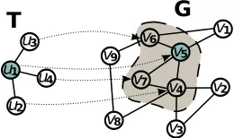
T with the root ρ(T) mapped to node f(ρ(T)). Figure 1 shows an example of a non-induced embedding of template
T in a graph G. Let emb(T, G) denote the number of all embeddings of template T in graph G. Here, we focus on approximatingemb(T, G).
G
T
v1v2
v3 v6 v9
v8 v7
v5
v4 u1
u2 u3
[image:3.612.373.503.490.567.2]u4
Fig. 1: Here the shaded subgraph is a non-induced embed-ding of T. The mapping of the template to the subgraph is denoted with the arrow.
An (ε, δ)-approximation to emb(T, G). We say that a
randomized algorithm A produces an (ε, δ)-approximation
to emb(T, G), if the estimate Z produced by A satisfies:
Pr[|Z−emb(T, G)|> ε·emb(T, G)]≤2δ; in other words,A
is required to produce an estimate that is close toemb(T, G), with high probability.
Problems studied.We consider the following two problems:
1) Subgraph counting: Given a template T and graph G,
IEEE TRANSACTIONS ON MULTI-SCALE COMPUTING SYSTEMS 4
Unlabeled Subgraph Countingproblem. Otherwise, it is
referred to as theLabeled Subgraph Countingproblem.
2) Graphlet Frequency Distribution (GFD)[28]: a graphlet is
another name for a subgraph. We say a node touches a graphletT, if it is contained in an embedding ofT
in the graphG. The graphlet degree of a nodevis the number of graphlets it touches. Given a size parameter
k, the GFD in a graphGis the frequency distribution of the graphlet degrees of all nodes with respect to all graphlets of size up to k. The specific problem is to obtain an approximation to the GFD. In this paper, we will focus on “treelets”, which only considers all trees of size up tok.
3.2 MapReduce, Hadoop and Harp
MapReduce and its extensions have become a dominant computation model in big data analysis. It involves two stages for data processing: (a) dividing the input into dis-tinct map tasks and distributing to multiple computing entities, and (b) merging the results of individual computing entities in thereducetasks to produce the final output [11].
The MapReduce model processes data in the form of key-value pairs hk, vi. An application first takes pairs of the form hk1, v1i as input to the map function, in which
one or more hk2, v2i pairs are produced for each input
pair. Then the MapReduce re-organizes allhk2, v2ipairs and
aggregates all itemsv2that are associated with the same key k2, which are then processed by a reduce function.
Hadoop [39] is an open-sourced implementation of MapReduce. By defining application specific map and re-duce functions, the user can employ Hadoop to manage and allocate appropriate resources in order to perform the tasks, without knowing the complexity of load balancing, communication and task scheduling. Due to the reliability and scalability in handling vast amount of computation in parallel, Hadoop is becoming a de facto solution for large parallel computing tasks.
Hadoop falls short in two aspects though: (i) the high I/O cost involved within the mapper, shuffling and the reducer since the data is always read and write from the disk in every stage of a Hadoop job and (ii) global synchro-nization of the mapper and reducer, i.e. reducers can start only when all mappers have completed their tasks and vice versa, thus reducing the efficient usage of the computing resources. To conquer the problems that Hadoop is facing, we further extend our work to use the Harp platform [29].
Harp introduces full collective communication (broad-cast, reduce, allgather, allreduce, rotation, regroup or push & pull), adding a separate communication abstraction. The advantage of using in-memory collective communication replacing the shuffling phase is that fine-grained data align-ment and data transfer of many synchronization patterns can be optimized.
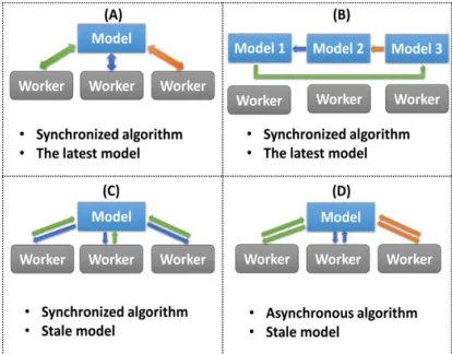
[image:4.612.334.541.43.205.2]Harp categorizes four types of computation models (Locking, Rotation, Allreduce, Asynchronous) that are based on the synchronization patterns and the effectiveness of the model parameter update. They provide the basis for a systematic approach to parallelizing iterative algorithms. Figure 2 shows the four categories of the computing model. The Harp framework has been used by 350 students at Indiana University for their course projects. Now it has
Fig. 2: Harp has 4 computation models: (A) Locking,(B) Rotation, (C) AllReduce, (D) Asynchronous
been released as an open source project that is available at the public github domain [1]. Harp provides a collection of iterative machine learning and data analysis algorithms (e.g. Kmeans, Multi-class Logistic Regression, Random Forests, Support Vector Machine, Neural Networks, Latent Dirichlet Allocation, Matrix Factorization, Multi-Dimensional Scal-ing) that have been tested and benchmarked on OpenStack Cloud and HPC platforms including Haswell and Knights Landing architectures. It has also been used for Subgraph mining, Force-Directed Graph Drawing, and Image classifi-cation appliclassifi-cations.
4
T
HE SEQUENTIAL ALGORITHM: C
OLORC
ODINGTABLE 1: Notations
symbol description symbol description
G graph T , T0, T00 template and sub-templates
n, m # nodes, # edges k # nodes inT
ρ root ofT S, si color set, theithcolor
d(v) degree of nodev N(v) neighbors of nodev
We briefly introduce the color coding algorithm for subgraph counting [5], which gives a randomized approx-imation scheme for counting trees in a graph. Some of the notation used in the paper is listed in Table 1.
High level description.There are two main ideas
underly-ing the color codunderly-ing algorithm of [5].
1) Colorful embeddings:
Color the nodes of the graph with k colors where
k ≥ |VT|, and only count “colorful” embeddings—an
embeddingH of the templateT is colorful if each node in H has a distinct color. The advantage of this is that the number of colorful embeddings can be counted by a simple and natural dynamic program.
a) In particular, letC(v, T(ρ), S)be the number of color-ful embeddings ofT with nodev∈VGmapped to the
rootρ, and using the color setS, where|VT|=|S|.
b) Suppose(ρ = u1, u2)is an edge incident on the root
c) SupposeS1 andS2 are disjoint subsets of colors such
that |S1| = |VT1|, |S2| = |VT2|. Let H1 and H2 be
two colorful embeddings ofT1andT2using color sets S1 and S2, respectively, with ρ1 and ρ2 mapped to
neighboring nodesv1 ∈VG andv2 ∈VG, respectively.
Then,H1andH2must benon-overlapping, because they
have distinct colors. d) Therefore,
C(v1, T, S) =
X
v2∈N(v1)
X
S=S1∪S2
C(v1, T1(v1), S1)·
C(v2, T2(v2), S2),
where the first summation is over all neighborsv2ofv1
and the second summation is over all partitionsS1∪S2
ofS.
2) Random colorings: If the coloring is done randomly with
k=|VT|colors, there is a reasonable probability kk!k that
an embedding is colorful—this allows us to get a good approximation of the number of embeddings.
Algorithm 1The sequential color coding algorithm.
1: Input:GraphG= (V, E)and templateT = (VT, ET)
2: Output:Approximation toemb(T, G)
3:
4: For each v ∈ VG, pick a color c(v) ∈ S = {1, . . . , k}
uniformly at random, wherek=|VT|.
5: Partition the treeT into subtrees recursively to form a setT using algorithm PARTITION(T(ρ)). For each tree
T0 ∈ T, we have a root ρ0. Furthermore, if |VT0| > 1, T0is partitioned into two treesT10, T20with rootsρ01=ρ0
andρ02, respectively, which are referred to as the active and passive children ofT0.
6: For eachv∈VG,Ti∈ T with rootρi, and subsetSi⊆S,
with|Si| =|Ti|, we computeC(v, Ti(ρi), Si)using the
the recurrence ( 1) below:
c(v, Ti(ρi), Si) =1d X
u X
c(v, Ti0(ρi), Si0)·
c(u, Ti00(τi), Si00),
(1)
wheredis equal to one plus the number of siblings ofτi
which are roots of subtrees isomorphic toTi00(τi).
7: For thejth random coloring, let
C(j)=1
q k! kk
P
v∈VGc(v, T(ρ), S), (2)
whereqdenotes the number of nodeρ0 ∈VT such that T is isomorphic to itself whenρis mapped toρ0.
8: Repeat the above steps N = O(eklog(1/δ)ε2 ) times,
and partition N estimates C(1), ..., C(N) into t = O(log(1/δ))sets. LetZj be the average of setj. Output
the median ofZ1, ..., Zt.
Algorithm 1 describes the sequential color coding algo-rithm. Figure 3 gives an example of computing Eq. 1.
5
P
ARALLEL ALGORITHMSIn this section, we present a parallelization of the color coding approach using MapReduce framework, we will first describe SAHAD [42], followed by EN-SAHAD and HARPSAHAD+ respectively.
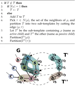
Algorithm 2Partition(T(ρ))
1: ifT /∈ T then
2: if|VT|= 1then
3: T ←T
4: else
5: AddT toT
6: Pickτ ∈ N(ρ), the set of the neighbors ofρ, and partition T into two sub-templates by cutting the edge(ρ, τ)
7: Let T0 be the sub-template containing ρ (name as
active child) andT00the other (name aspassive child)
8: Partition(T0(ρ))
[image:5.612.314.565.54.342.2]9: Partition(T00(τ))
Fig. 3: The example shows one step of the dynamic programming in color coding. T in Figure 1 is split into T0 and T00. To count C(w
1, T(v1), S), or
the number of embeddings of T(v1) rooted at w1,
using color set S = {red, yellow, blue, purple, green}, we first obtain C(w1, T0(v1),{r, y, b}) = 2 and C(w5, T00(v3),{p, g}) = 1. Then, C(w1, T(v1), S) =
C(w1, T0(v1),{r, y, b})C(w5, T00(v3),{p, g}) = 2.
The embeddings of T are subgraphs with nodes
{w3, w4, w1, w5, w6} and {w3, w2, w1, w5, w6}. Here
s, c, b represents the label of the nodes. Details of labeled
subgraph counting can be found at [42].
5.1 SAHAD
SAHAD takes a sequence of templates T = {T0, ..., T}
as input. Here T represents a set of templates generated by partitioning T using Algorithm 2. Then it performs a MapReduce variation of Algorithm 1 to compute the num-ber of embeddings ofT.
As shown in Equation 1, the counts of all colorful em-beddings isomorphic to T rooted from a single node v is computed by aggregating the same measurement ofT0and
T00, i.e., the two sub-templates, withT0 rooted fromv and
T00rooted from∀u∈N(v). We can parallelize color-coding algorithm by distributing the computation among multiple machines, and sending data related withv andN(v) to a computation unit for the aggregation. In our MapReduce algorithm, we manage this by assigning v as the key for both the counts ofT0rooted atvand the counts ofT00rooted
atv’s neighbors, such that all data required for computing counts for T rooted at v has the same key and will be handled by a single reduce function.
IEEE TRANSACTIONS ON MULTI-SCALE COMPUTING SYSTEMS 6
{s0
1, s02, ..., s0k}, c0),(S1 = {s11, s12, ..., s1k}, c1), ..., where Si
represents a color set containingkcolors, andcirepresents
the counts of the subgraphs isomorphic toT and rooted atv
that are colored bySi. Herek=|V(T)|, and each subgraph
is a colorful match.
There are 3 types of Hadoop jobs in SAHAD, which are 1) colorer (Algorithm 3) that performs line 4 of Algorithm 1; 2) counter (Algorithm 4, 5) which performs line 6 of Algorithm 1 and 3) finalizer (Algorithm 6, 7) that performs line 7 of Algorithm 1.
The first step is to random color networkGwithkcolors. The map function is described in Algorithm 3:
Algorithm 3mapper(v, N(v))
1: Picksi∈ {s1, . . . , sk}uniformly at random
2: colorvwithsi
3: LetT0be the single node template
4: Letc(v, T0,{si}) = 1sincevis the only colorful
match-ing
5: XT0,v← {({si},1)}
6: Collect(key←v, value←XT0,v, N(v))
Here “Collect” is a standard MapReduce operation that will emit the key-value pairs to global space for further process such as shuffling, sorting or I/O. N(v)represents the neighbors ofv. Note that templateT0 is a single node,
therefore XT0,v contains only a single color-count pair
(sv,1)
According to Equation 1, to compute XTi,v, we need
XT0
i,v for sub-templateT 0
i and XT00
i,u for allu ∈ N(v)for
sub-templateTi00. We use a mapper and a reducer function to implement this as shown in Algorithm 4 and 5, respectively.
Algorithm 4mapper(v, Xt,v, N(v))
1: iftisTi0then
2: Collect(key←v, value←Xt,v, f lag0)
3: else
4: foru∈N(v)do
5: Collect(key←u, value←Xt,v, f lag00)
Note that in Algorithm 4, the secondCollectemitsXT00 i,v
to all its neighbors. Therefore, as shown in Algorithm 5,
XT0
i,vandXT
00
i,ufrom allu∈N(v)are handled by the same
reducer, which is sufficient for computing Eq. 1. Also note that for a given nodev, the number of entries withf lag0 is 1, and the number of entries withf lag00equals|N(v)|.
Algorithm 5reducer(v,(X, f lag),(X, f lag), ...)
1: pickX1wheref lag=f lag0
2: forall colorsetSi0fromX1do
3: foreachX other thanX1do
4: forall colorsetSi00fromX do
5: ifSi0∩Si00=∅then
6: c(v, Ti, Si0∪Si00)+ = 1
7: Collect(key←v, value←XTi,v, N(v))
The last step is to compute the total count described in Eq. 2, and is shown in Algorithm 6 and 7.
Algorithm 6mapper(v, XT ,v, N(v))
1: Collect(key←“sum00, value←XT ,v)
Algorithm 7reducer(“sum00, XT ,v1, XT ,v2, ...)
1: Y = mm!m ·1 q
P
∀v∈VGX
2: Collect(key←“sum00, value←X T ,v)
Note that in Algorithm 6, XT ,v only contains one
ele-ment, which is the count corresponding to the entire color set. Then in the reducer shown in Algorithm 7, all the counts are added together and properly factorized, to obtain the final count. For a comprehensive description of the MapReduce version of color coding, please refer to [42].
5.2 EN-SAHAD
For general MapReduce problem, the set of keys that is processed in the Mapper and Reducer varies among dif-ferent jobs. Therefore, MapReduce uses external shuffling and sorting in-between Mappers and Reducers to deploy the keys to computing nodes.
In our algorithm, however, the dynamic program aggre-gates counts based on the root node of the subtree, and therefore the key is the node indexv. In EN-SAHAD, we use this pre-knowledge to predefine a reducer that corresponds to a set of nodes. We also assign the predefined reducers to computing nodes prior to the beginning of the dynamic program. Therefore, a data entry with keyvwill be directly sent to the corresponding computing node and processed by designated Reducer. Using this mechanism, we can reduce the cost of shuffling and sorting in intermediate stage of Hadoop jobs.
5.3 HARPSAHAD+
HARPSAHAD+ is built upon the Harp framework [?] [?], which adopts a variety of the advanced technologies in the research area of high performance Java language. HARP -SAHAD+ has the following optimization in front of the MapReduce Sahad version: 1) It uses a two-level parallel programming model. At the inter-node level, workload is distributed by harp mappers; At the intra-node level, local workload is divided and assigned to multiple Java threads. 2) For inter-node communication, it utilizes a MPI-AlltoAll like regroup operation owned by Harp. 3) For intra-node computation, it utilizes Habanero Java thread library from Rice University [?] and adopts a Long-Running-Thread pro-gramming style [?] to unleash the potential performance of Java language.
5.3.1 Inter-Node Communication
we create a table LT able with si entries, and each entry
0 ≤j < si serves as a “reducer” for vertexvj. HARP
SA-HAD+ then uses a regroup operation to “shuffle” the data within the memory but in a collective way. Each mapper function creates another harp Table objectRT able, contain-ing multiple partitions, to transfer data. A preprocesscontain-ing function is fired to record re-usable information required by regroup operations in each iteration. In the preprocessing stage, each mapper holds a copy of all the vertex IDsvand the mapper ID j, v ∈ Vj by an allgather communication
operation. The mapper then parses the neighbour listsN(v) of all the local verticesViand labels each vertexu,u∈N(v)
butu /∈Vi, with a mapper IDjthatu∈Vj. Therefore, each
mapperikeeps a queue of vertex IDs for each mapperj6=i
with∀v∈Qi,j, v∈Vj. By sendingQi,jto mapperj, finally
each mapperjobtains a sending queueQj,iof vertices.
In each iteration of HARPSAHAD+, the regroup opera-tion fired by mapperihas three steps: 1) For each sending queue Qi,j, loading subtemplate counts of v in sending
queueQi,jinto a partitionP ari,jofRT able. 2) The sender
and receiver mapper identities, i and j, are coded into a single partition ID forP ari,j. During the collective
regroup-ing, a designed harp partitioner will decode the partition ID and deliver the partitionP ari,j to the receiver mapper j. 3) After the regroup operation, the harp TableRT ableof each mapperinow contains counts of verticesu∈N(v)to update subtemplate counts of local verticesvinLT able.
5.3.2 Intra-Node Computation
HARPSAHAD+ extends the MapReduce framework by tak-ing advantage of the multi-threadtak-ing programmtak-ing model in a shared-memory node. We favor the Habanero Java threads instead of the Java.lang.Thread implementation be-cause it allows users to setup thread affinity in multi-core/many-core processors. We also embrace the so-called Long-Running-Thread programming style, where we create the threads at the most out loop and keep them running until the end of the program. This approach avoids the overhead of frequently creating and destroying threads, instead, it uses java.util.concurrent.CyclicBarrier object to synchronize threads if required.
6
P
ERFORMANCEA
NALYSISIn this section, we discuss the performance of SAHAD in terms of the overall work and time complexity. Throughout this section, we denote the number of nodes and edges in the network bynandmrespectively. We usekto represent the number of nodes in the template.
Lemma 6.1.For a templateTi, suppose the sizes of the two
sub-templates Ti0 and Ti00 are ki0 and k00i, respectively. As a result, the sizes of the input, output, and work complexity corresponding to a nodevare given below:
• The sizes of the input and output of Algorithm 4 are
O( kk0 i
+ kk00 i
+d(v))andO( kk00 i
d(v)), respectively.
• The size of the input to Algorithm 5 isO( kk00 i
d(v)).
Proof For a nodev, the input to Algorithm 4 involves the
correspondingXT0
i,v and XTi00,v for T
0
i andTi00, as well as N(v), which together have sizeO( kk0
i
+ kk00 i
+d(v)). If the
input is forTi00, Algorithm 4 generates multiple key-value pairs for a nodev, in which each key-value pair corresponds to some node u ∈ N(v). Therefore, the output has size
O( kk00 i
d(v)).
For a given v, the input to Algorithm 5 is the combina-tion of the above, and therefore, has sizeO( kk00
i
d(v)).
Lemma 6.2. The total work complexity is
O(k|EG|22keklog (1/δ)ε12).
Proof For nodevand each neighboru∈N(v), Algorithm 5
aggregates every pair of the form (Sa, Ca) in XT0 i,v, and
(Sb, Cb) in XT00
i,u, which leads to a work complexity of O( kk0
i
k
k00 i
d(v)). Since |T | ≤ k, the total work, over all nodes and templates is at most
O(X
v,Ti k k0i
! k k00i
!
d(v)) =O(X
v
k22kd(v)) =O(k|EG|22k)
(3) SinceO(eklog (1/δ)1
ε2)iterations are performed in order
to get the(ε, δ)-approximation, the lemma follows.
Time Complexity. We use P to denote the number of
machines. We assume each machine is configured to run a maximum ofM Mappers andRReducers simultaneously. Finally, we assume a uniform partitioning, so that each machine processesn/P nodes.
Lemma 6.3. The time complexity of Algorithm 3 and 4 is
O(P Mn )andO(P Mm ), respectively.
Proof We first consider Algorithm 3, which takes as input
an entry of the form(v, N(v))for some node v, and per-form a constant work. There are Pn entries processed by each machine. Since M Mappers are run simultaneously, this gives a running time of O(P Mn ). Next, we consider Algorithm 4. Each Mapper outputs(v, X)for inputTi0 and
d entries for input T00
i for each u ∈ N(v), where d is
the degree ofv. Therefore, each computing node performs
O(Pn/Pi=1 di) = O(m/P) steps. Here di is the degree for vi. Again, since M Mappers run simultaneously, the total
running time isO(P Mm ).
Lemma 6.4.The time complexity of Algorithm 5 isO(m·2P R2k).
Proof Suppose |Si0| = k0i and |S00i| = k00i. The number of possible color setsSi0 andSi00 is kk0
i
and kk00 i
, respectively. Line 2 of Algorithm 5 involves O( kk0
i
) = O(2k) steps.
Similarly, line 4 also involves O(2k)
steps and Line 3 in-volves O(d) steps. Therefore the totally running time is
O(d)·22k. Each machine processes n
P entries corresponding
to different nodes, leading to a total ofO(nd·2P2k)steps. Since
Rreducers run in parallel on each machine, this leads to a total time ofO(m·2P R2k).
Lemma 6.5. The time complexity of Algorithm 6 and 7 is
O(P Mn )andO(n), respectively.
Proof Algorithm 6 maps out a single entry for each input.
IEEE TRANSACTIONS ON MULTI-SCALE COMPUTING SYSTEMS 8 have only one key “sum”, and only one Reducer will be
assigned for the summation for allv ∈ V(G), which takes
O(n)time.
Lemma 6.6.The overall running time of SAHADis bounded
by
O(k22Pkm·(M1 +R1)eklog (1/δ)1
ε2) (4)
Proof Algorithm 3 takes O(P Mn ) time. Algorithm 4 and
5 run for each step of the dynamic programming, i.e., joining two sub-templates into a larger template as shown in Figure 3. Since the number of total sub-templates is
O(k) when T is a tree, Algorithm 4 and 5 run O(k) times. Therefore the total time is O(k·(P Mm + m·2P R2k)) =
O(k22Pkm·(M1 + R1). Finally, the entire algorithm as to be repeatedO(eklog (1/δ)1
ε2)times, in order to get the (ε, δ)
-approximation, and the lemma follows.
6.1 Performance Analysis of Intermediate Stage
[image:8.612.70.280.349.448.2]With SAHAD, a major bottleneck of a Hadoop job in terms of running time is the shuffling and sorting cost in the intermediate stage between Mapper and Reducer, due to the high I/O and synchronization cost as shown by the black bar in Figure 4.
Fig. 4: The figure shows the time spent in each stage of a running Hadoop job to produce a color-count for a 5-node template, by aggregating the 2-node and 3-node sub-tree. The black bar is the time for the intermediate stage, which is for shuffling and sorting.on which graph is this?
We observe that the external shuffling and sorting stage takes roughly twice the time of the reducing stage, which dramatically increase the overall running time. Given that the keys in Mappers and Reducers are always the index of all the nodes v ∈ V(G), we can enhance SAHAD by re-moving the shuffling and sorting in the intermediate stages. Instead, we can designate Reducers and directly send the data to corresponding Reducers.
7
V
ARIATIONS OFS
UBGRAPHI
SOMORPHISMP
ROBLEMSSo far we have discussed the basic framework of the al-gorithm. We have also discussed how to compute the total number of subgraph embeddings in Algorithm 7. We now discuss a set of problems that are closely the subgraph isomorphism problem, including finding supervised motif and computing graphlet frequency distribution, which can be computed using our framework.
Note that our algorithm is specifically suitable for com-puting on multiple templates if they have common sub-templates, since those common sub-templates only need to be computed once. This is the case in many problems, where common sub-templates such as single node, edge, or simple paths are shared.
7.1 Supervised Motif Finding
Motifs of a real-world network are specific templates whose embeddings occur with much higher frequencies than in random networks and are referred as building blocks for networks. They have been found in many real-world net-works [26]. Our algorithm can reduce the computational cost for a group of templates since the common sub-templates are only computed once, therefore, this approach is amenable to be applied in supervised motif finding.
7.2 Graphlet Frequency Distribution
Graphlet frequency distribution has been proposed as a way of measuring the similarity of protein-protein networks [28], where common properties such as degree distribution, di-ameter, etc., may not suffice. Unlike “motifs”, graphlet frequency distribution is computed on all selected small subgraphs regardless of whether they appear frequently or not.
Graphlet frequency distribution D(i, T) measures the number of nodes from whichigraphlets that are isomorphic toTare touched on. The number of graphlets touched on a single nodevcan be computed using a number of counts of the same templatesT with root placed at different nodes of
T.
8
E
XPERIMENTALA
NALYSIS OFSAH
AD, E
N-SAH
AD& H
ARPSAH
AD+
We carry out a detailed experimental analysis of SAHAD, EN-SAHAD and HARPSAHAD+, by focusing on three as-pects:
(i) Quality of the solution: We compare the color coding
results with exact counts on small graphs in order to mea-sure the empirical approximation error of our algorithms and show that the error is very small (less than 0.5% with one iteration as shown in Figure 7) so in the following experiments we run the program for a single iteration.
(ii)Scalability of the algorithms as a function of template size,
graph size and computing resources: We carried out
experi-ments using templates with sizes ranging from 3 nodes to 12 nodes, including both labeled and unlabeled templates. The graphs we use go from several hundreds of thousands of nodes to tens of millions. We also study how our algorithm scales in terms of computing resources including number of threads per node, number of computing nodes, as well as different settings of mappers and reducers, etcetera.
(iii) Variations of the problem: Our framework has the
ability to extend to a variety of measurements related with the subgraph counting problem. In the experiments, we show the unlabled/labeled subgraph counting and graphlet distribution results.
(iv) Enhancing overall performance by system tuning: We
their impact to the overall performance. For example, EN
-SAHADstudies the communication and sorting cost in the intermediate stage of the system and gives approaches for improvement. We also propose a degree based graph parti-tioning scheme that can improve the performance of Harp by imposing better load balancing in terms of computations within each partition. Table 2 highlights the main results we obtained with various methods.
TABLE 2: Comparison on SAHAD, EN-SAHADand HARP -SAHAD+
Method Networks Templates Performance
SAHAD 268M edges ≤12 nodes 10s of min for 7 node
template on Chicago
EN-SAHAD 12M edges 5 nodes 20% improvement
over SAHAD
HARPSAHAD+ 1.2B edges up to 12 nodes 100-200 times faster
than SAHAD
8.1 Experiment Design
8.1.1 Datasets
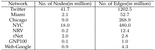
[image:9.612.307.566.44.132.2]For our experiments, we use synthetic social contact net-works of the following cities and regions: Miami, Chicago, New River Valley (NRV), and New York City (NYC) (see [7] for detains). We consider demographic labels –{kid, youth, adult, senior} based on the age and gender for individu-als. We also run experiments on a G(n, p) graph (denoted GNP100) withnnodes, where each pair of nodes are con-nected with probabilityp, and are randomly assigned node labels. We also experiment on a few other networks: Web-Google [2], RoadNet (rNet) [2], Twitter [21] and Chung-Lu random graphs [9]. Table 3 summarizes the characteristics of the networks.
TABLE 3: Networks used in the experiments
Network No. of Nodes(in million) No. of Edges(in million)
Twitter 41.7 1202.5
Miami 2.1 52.7
Chicago 9.0 268.9
NYC 18.0 480.0
NRV 0.2 12.4
rNet 2.0 2.8
GNP100 0.1 1.0
Web-Google 0.9 4.3
8.1.2 Templates
The templates we use in the experiments are shown in Figure 5. The templates vary in size from 5 to 12 nodes, in whichU5-1,. . .U10-1are the unlabeled templates and
L7-1 ,L10-1 as well as L12-1 are the labeled templates. In the
labels, m,f, k, y, a and s stand for male,female,kid,youth,
adultandsenior, respectively.
8.1.3 Computing Environment
For experiments with SAHAD, we use a computing cluster
Athena, with 42computing nodes and a large RAM
mem-ory footprint. Each node has a quad-socket AMD 2.3GHz Magny Cour 8 Core Processor, i.e., 32 cores per node or 1344 cores in total, and 64 GB RAM(12.4 TFLOP peak). The local disk available on each node is750GB. Therefore,
U5-1 U5-2 U5-3 U7-1 U10-1
L7-1 L10-1
ms
ma fa
fa my
my fy
fk
fy fy
fy
fy fa
fa fs fa
fs L12-1
mk
ma
ms mk
ms
my fk
fk my
mk ms
ma
Fig. 5: Templates used in the experiments.
we can have maximum 31.5T B storage for the HDFS. In most of our experiments, we use up to 16 nodes, which give up to 12T B capacity for the computation. Although the number of cores and RAM capacity on each node can support a large number of mappers/reducers, the avail-ability of a single disk on each node limits aggregate I/O bandwidth of all parallel processes on each node. To make it worse, aggregate I/O bandwidth of parallel processes doing sequential I/O could result in many extra disk seeks and hurt overall performance. Therefore, disk bandwidth is the bottleneck for more parallelism in each node. This limitation is further discussed in section 8.2.2. We also use the public Amazon Elastic Computing Cloud (EC2) for some of our experiments. EC2 enables customers to instantly get cheap yet powerful computing resources, and start the computing process with no upfront cost for hardware. We allocated 4
High-CPU Extra-Largeinstances from EC2. Each instance has
8cores,7GB RAM, and two250GB virtual disks (Elastic Block Store Volume).
For experiments with HARPSAHAD+, we use the Juliet cluster (Intel Haswell architecture) with 1, 2, 4, 8 and 16 nodes. The Juliet cluster contains 32 nodes each with two 18-core 36-thread Intel Xeon E5-2699 processors and 96 nodes each with two 12-core 24-thread Intel Xeon E5-2670 processors. All the nodes used in the experiments are with Intel Xeon E5-2670 processors and 128 GB memory. All the experiments are performed on InfiniBand FDR with 10Gbit/s per link.
8.1.4 Performance metrics
We carry out experiments on SAHAD, EN-SAHAD and HARPSAHAD+. For SAHAD, we measure the approxima-tion bounds, the impact of Hadoop configuraapproxima-tion including number of Mapper/Reducers and performance on queries related with various templates and graphs. For enhanced SAHAD, we measure the performance improvement gained by eliminating the sorting in the intermediate stage. We also measures the impact with difference partitioning schemes. Then with Harp, similar to SAHAD, we measure the perfor-mance impact with various templates and graphs, as well as the system performance regarding number of computing nodes. We also compare HARPSAHAD+ and SAHAD to
study the improvement Harp brings.
8.2 Performance of SAHAD
[image:9.612.46.303.461.545.2]IEEE TRANSACTIONS ON MULTI-SCALE COMPUTING SYSTEMS 10
1. Approximation bounds: While the worst case bounds
on the algorithm implyO(eklog (1/δ)ε12)rounds to get an
(ε, δ)-approximation (see Lemma 6.2), in practice, we find that far fewer iterations are needed.
2. System performance: We run our algorithm on a
diverse set of computing resources, including the publicly available Amazon EC2 cloud. Here, we find that our algo-rithm scales well with the number of nodes, and disk I/O is one of the main bottlenecks.We posit that employing multiple disks per node (a rising trend in Hadoop) or using I/O caching will help mitigate this bottleneck and boost performance even further.
3. Performance on various queries: We evaluate the
performance on templates with sizes ranging from 5 to 12. Here, we find that labeled queries are significantly faster than unlabeled ones, and the overall running time is under 35 minutes for these queries on our computing cluster (described below). We also get comparable performance on EC2.
8.2.1 Approximation bounds
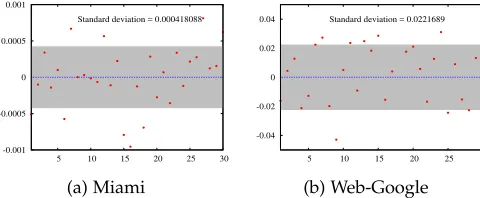
As discussed in Section 3, the color coding algorithm aver-ages the estimates over multiple iterations. Figure 6 shows the error for each iteration in countingU5-1for Miami and Web-Google, respectively. It is observed that the standard deviation for the error is 2% and 0.4% for Miami and Web-Google, which is very small.
-0.001 -0.0005 0 0.0005 0.001
5 10 15 20 25 30
Standard deviation = 0.000418088
(a) Miami
-0.04 -0.02 0 0.02 0.04
5 10 15 20 25 30 Standard deviation = 0.0221689
[image:10.612.58.298.362.461.2](b) Web-Google
Fig. 6: Error in countingU5-1for 30 iteration
In Figure 7, we show that the approximation error is below0.5% for the template U7-1 for the GNP100 graph, even for one iteration. The figure also plots the results based on using more than 7 colors, which can sometimes improve the running time, as discussed in [16]. In the rest of the experiments, we only use the estimation from one iteration, because of the small error shown in this section. The error foriiterations is computed using |(
P
iZi)/i−emb(T ,G)|
emb(T ,G) .
0 0.002 0.004 0.006 0.008 0.01
1 2 3 4 5 6 7 8
error
[image:10.612.315.566.462.552.2]number of iterations size of colorset = 7 size of colorset = 8 size of colorset = 9 size of colorset = 10 size of colorset = 11
Fig. 7: Approximation er-ror in counting U7-1 on GNP100.
0 50 100 150 200 250
2 4 6 8 10 12 14
running time (min)
number of computing nodes Miami GNP100
Fig. 8: Running time for countingU10-1vs number of computing nodes.
8.2.2 Performance Analysis
We now study how the running time is affected by the number of total computing nodes and number of reduc-ers/mappers per node. We carry out 3 sets of experiments: (i) how the total running time scales with the number of computing nodes; (ii) how the running time is affected by varying assignment of mappers/reducers per node.
1. Varying number of computing nodesFigure 8 shows
that the running time for Miami reduces from over 200 minutes to less than 30 minutes when the number of com-puting nodes increases from 3 to 13. However, the curve for GNP100 does not show good scaling. The reason is that the actual computation for GNP100 only consumes a small portion of the running time, and there is overhead from managing the mappers/reducers. In other words, the curve for GNP100 shows a lower bound on the running time in our algorithm.
2.Varying number of mappers/reducers per nodeHere
we consider two cases.
2.a. Varying number of reducers per node. Figure 9 shows
the running time on Athena when we vary the number of reducers per node. Here we fix the number of nodes to be 16 and the number of mappers per node to be 4. We find that running 3 reducers concurrently on each node minimizes the total running time. In addition we find that although increasing the number of reducers per node can reduce the time for the Reduce stage for a single job, the running time increases sharply in Map and Shuffle stage. As a result, the total running time increases with the number of reducers. This can be explained by the visible I/O bottleneck for concurrent accessing on Athena, since Athena has only 1 disk per node. This phenomenon is not present on EC2, as seen from Figure 11b, indicating that EC2 is better optimized for concurrent disk accessing for cloud usage.
0 20 40 60 80 100 120
0 2 4 6 8 10 12 14 16 18
running time (min)
number of reducers per node
(a) Total running time v.s. num-ber of reducers.
0 5 10 15 20 25
0 2 4 6 8 10 12 14 16 18
running time (min)
number of reducers per node mapper shuffle and sorting reducer
(b) Running time of job stages v.s. number of reducers.
Fig. 9: Running time v.s. number of reducers per node
2.b. Varying number of mappers per node.Figure 10 shows
the running time on Athena when we vary the number of mappers per node while fixing the number of reducers as 7 per node. We find that varying the number of mappers per node does not affect the performance. This is also validated in EC2, as shown in Figure 11.
2.c. Reducers’ running time distribution. Figure 12 shows
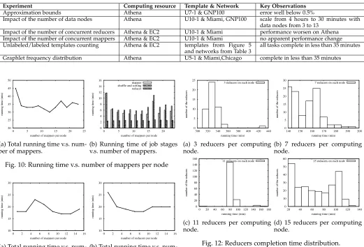
[image:10.612.51.301.601.687.2]TABLE 4: Summary of the experiment results (refer to Section 8.1 for the terminology used in the table)
Experiment Computing resource Template & Network Key Observations
Approximation bounds Athena U7-1 & GNP100 error well below 0.5%
Impact of the number of data nodes Athena U10-1 & Miami, GNP100 scale from 4 hours to 30 minutes with
data nodes from 3 to 13
Impact of the number of concurrent reducers Athena & EC2 U10-1 & Miami performance worsen on Athena
Impact of the number of concurrent mappers Athena & EC2 U10-1 & Miami no apparent performance change
Unlabeled/labeled templates counting Athena & EC2 templates from Figure 5
and networks from Table 3
all tasks complete in less than 35 minutes
Graphlet frequency distribution Athena U5-1 & Miami,Chicago complete in less than 35 minutes
20 25 30 35 40 45 50
0 5 10 15 20 25
running time (min)
number of mappers per node
(a) Total running time v.s. num-ber of mappers.
0 2 4 6 8 10 12 14 16
0 5 10 15 20
running time (min)
number of mappers per node mapper shuffle and sorting reducer
[image:11.612.50.571.56.410.2](b) Running time of job stages v.s. number of mappers.
Fig. 10: Running time v.s. number of mappers per node
10 15 20 25 30
0 2 4 6 8 10 12 14 16
running time (min)
number of mappers per node
(a) Total running time v.s. num-ber of mappers on EC2.
10 15 20 25 30
0 2 4 6 8 10 12 14 16
running time (min)
number of reducers per node
[image:11.612.314.566.428.507.2](b) Total running time v.s. num-ber of reducers on EC2.
Fig. 11: Running time w.r.t. number of mappers and reduc-ers on EC2.
This also indicates the bad I/O performance on Athena for concurrent accessing.
8.2.3 Illustrative applications
In this section, we illustrate the performance on3different kinds of queries. We use Athena and assign 16 nodes as the data nodes; for each node, we assign a maximum of 4 mappers and3reducers per node. Our experiments on EC2 for some of these queries are discussed later in Section 8.2.4.
1. Unlabeled subgraph queries: Here we compute the
counts of templatesU5-1,U7-1andU10-1on GNP100 and Miami, as well as the running time, as shown in Figure 13 – we observe that for unlabeled templates with up to 10 nodes on the Miami graph, the algorithm runs in less than 25minutes.
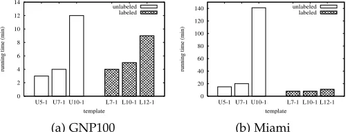
2. Labeled subgraph queries: Here we count the total
number of embeddings of templatesL7-1,L10-1andL12-1in Miami and Chicago. Figure 14b shows that the running time for counting templates up to12nodes is around15minutes on Miami, which is less than35minutes needed for Chicago. The running time is much less for the labeled subgraph queries than that for the unlabeled subgraph queries. This is
0 5 10 15 20 25
300 320 340 360 380 400 420 440
number of the reducers
running time (min) 3 reducers on each node
(a) 3 reducers per computing node.
0 5 10 15 20 25 30
140 150 160 170 180 190 200
number of the reducers
running time (min) 7 reducers on each node
(b) 7 reducers per computing node.
0 20 40 60 80 100 120 140 160
0 20 40 60 80 100 120 140 160 180
number of the reducers
running time (min) 11 reducers on each node
(c) 11 reducers per computing node.
0 10 20 30 40 50 60
20 40 60 80 100 120 140
number of the reducers
running time (min) 15 reducers on each node
(d) 15 reducers per computing node.
Fig. 12: Reducers completion time distribution.
1e+08 1e+09 1e+10 1e+11 1e+12 1e+13 1e+14 1e+15 1e+16 1e+17
Miami GNP100
number of subgraph matchings
graph U5-1
U5-2 U5-3 U7-1 U10-1
(a) The counts of unlabeled sub-graphs.
0 5 10 15 20 25 30
Miami GNP100
running time (min)
graph U5-1
U5-2 U5-3 U7-1 U10-1
(b) Running time for counting unlabeled subgraphs.
Fig. 13: Querying unlabeled subgraphs on GNP100 and Miami
due to the fact that labeled templates contain a much fewer number of embeddings due to the label constraints.
3. Computing graphlet frequency distribution:
Fig-ure 15 shows the graphlet frequency distribution in the networks of Miami and Chicago, respectively. By using templateU5-1for this experiment, we observe that it takes 15 minutes and 35 minutes to compute graphlet frequency distributions on Miami and Chicago, respectively.
8.2.4 Performance Study with Amazon EC2
On EC2, we run unlabeled and labeled subgraph queries on Miami and GNP100 for templatesU5-1,U7-1,U10-1,L7-1,
IEEE TRANSACTIONS ON MULTI-SCALE COMPUTING SYSTEMS 12
1e+10 1e+11 1e+12 1e+13 1e+14 1e+15 1e+16
Chicago Miami
number of subgraph matchings
graph L7-1
L10-1 L12-1
(a) The counts of labeled sub-graphs.
0 5 10 15 20 25 30 35
Chicago Miami
running time (min)
graph L7-1
L10-1 L12-1
[image:12.612.52.301.47.129.2](b) Running time for counting labeled subgraphs.
Fig. 14: Querying labeled subgraphs on Miami and Chicago.
1 10 100 1000 10000 100000 1e+06
0 5e+08 1e+09 1.5e+09 2e+09 2.5e+09 3e+09
number of nodes
number of graphlet adjacent to a node Miami
(a) Miami
1 10 100 1000 10000 100000 1e+06
0 1e+09 2e+09 3e+09 4e+09 5e+09 6e+09
number of nodes
number of graphlet adjacent to a node Chicago
[image:12.612.313.566.164.263.2](b) Chicago
Fig. 15: Graphlet distribution on Miami and Chicago.
discussed previously, and each node runs up to a maximum of 2 mappers and 8 reducers concurrently. As shown in Figures 16, the running time on EC2 is comparable to that on Athena, except forU10-1on Miami, which takes roughly2.5 hours to finish on EC2, but only25minutes on Athena. This is because for large templates and graphs as large as Miami, the input/output data as well as the I/O pressure on disks is tremendous. EC2 uses virtual disks as local storage, which hurt overall performance when dealing with such a large amount of data.
0 2 4 6 8 10 12 14
L12-1 L10-1 L7-1 U10-1 U7-1 U5-1
running time (min)
template unlabeled
labeled
(a) GNP100
0 20 40 60 80 100 120 140
L12-1 L10-1 L7-1 U10-1 U7-1 U5-1
running time (min)
template unlabeled
labeled
[image:12.612.51.314.193.292.2](b) Miami
Fig. 16: Running time for various templates on EC2.
8.3 Performance of EN-SAHAD
In this section we experiment our algorithms on two real-world networks NRV and RoadNetand a number of their shuffled versions. We generate shuffled networks with 20, 40, 60, 80 and 100 percent shuffling ratio, and name them as
nrv20tonrv100, andrNet20torNet100.
As discussed in Section 5.2, a major factor that impacts the overall performance is the heavy shuffling and sorting cost in the intermediate stage of a Hadoop job. We mitigate this factor by designating node indexvto Reducers, and pre-allocating Reducers among computing nodes. In this way,
the key-value pairs from Mappers can be directly sent to corresponding Reducers without being shuffled and sorted. Figure 17 shows the overall running time of our algo-rithm onNRV,RoadNetand their variations. Here we gen-erate the variations of the graph by shuffling a proportion of the edges in the graph, e.g., nrv40 is a NRV with 40% of its edges being shuffled. As a result, we observe that pre-allocating a Reducer can deliver roughly a 20% performance improvement.
0 100 200 300 400 500
nrv nrv20 nrv40 nrv60 nrv80 nrv100
running time (sec)
graphs SAHad Enhanced-SAHad
(a) NRV and its variations
0 100 200 300 400 500
rnet rnet20 rnet40 rnet60 rnet80 rnet100
running time (sec)
graphs SAHad En-SAHad
(b) RoadNet and its variations
Fig. 17: SAHADv.s. EN-SAHADon RoadNet and NRV.
8.4 Performance of HARPSAHAD+
In the following experiments, we evaluate the performance of HARPSAHAD+ by comparing it with a state-of-the-art MPI subgraph counting program called Fascia. MPI-Fascia is developped by Slota et al. [34], which implements the same color coding algorithm as SAHAD and HARP -SAHAD+. MPI-Fascia uses a MPI+OpenMP programming model. In our tests, it is compiled with g++ 4.4.7 and compiler option -O3 as well as OpenMPI 1.8.1. Also, we choose InfiniBand instead of Ethernet as the interconnect to test MPI-Fascia and HARPSAHAD+, thus offering more challenges to the Java based communication operation of HARPSAHAD+.
8.4.1 Execution Time
In Figure 18a, we observe that HARPSAHAD+ has a 100x to 200x speedup over SAHAD on a single Haswell node. This tremendous improvement comes from two sides: 1) HARPSAHAD+ has a better utilization of the hardware
[image:12.612.51.304.465.561.2]Miami Web-Google 10
100 1,000
4 2 800 170 8 2 1200 260 Graphs R unning time (Sec) HarpSahad+ u5-1 SAHad u5-1 HarpSahad+ u7-1 SAHad u7-1
(a) SAHADvs. HARPSAHAD+
NYC Twitter
0 2,000 4,000 6,000
355
1,360 546
1,887 1,201
6,874
1,486
7,217
Graph R unning time (Sec) HarpSahad+ U10-1 MPI-Fascia U10-1 HarpSahad+ U12-2 MPI-Fascia U12-2
(b) HARPSAHAD+ vs. MPI-Fascia
Fig. 18: (a) Test on 1 Haswell Node and each node running 40 threads; (b) Test on 16 Haswell Nodes and each node running 24 threads
0 1,000 2,000 3,000 4,000 5,000 6,000 7,000 8,000
HarpSahad+ MPI-Fascia
Counting Time in Seconds
[image:13.612.52.299.47.146.2]Computation Communication
Fig. 19: BreakDown of Time for Twitter-U12-2 on 16 Nodes
8.4.2 Problem Size Scaling
Next we study the performance of HARPSAHAD+ by con-trolling the number of nodes in a graph while increasing the number of edges. In this experiment, we use the Chung-Lu model [9] to generate a series of random graphs given the degree sequence and its variations of Miami and NYC. The average degree of the generated random graphs range from 50 to 150 for Miami and 10 to 100 for NYC. In Figure 20, the running time generally increases with the number of edges, which meets the time complexity we propose in Section 6. For Miami, when the average degree increases from 50 to 150, the running time only increases by 1.7x. Also, a tenfold (x10) increase in average degree for the NYC graph only accounts for less than 2x of an increase in running time. This indicates that our HARPSAHAD+ implementation maintains good performance in computing the neighbours of vertices in parallel, which is due to the high efficiency of Java threads.
CL0 CL1 CL2 CL3 CL4 CL5 CL6 CL7 CL8 CL9 0 50 100 150 200 110 118 146 136 161 161 157
185 188 188
Graph Name Coun ting Time (sec) HarpSahad+
(a) Miami Dataset
CL0 CL1 CL2 CL3 CL4 CL5 CL6 CL7 CL8 CL9 0
200 400 600 800 1,000 1,200 1,400
712 777 886 956
1,0041,049 1,016 1,179
1,312 1,240
Graph Name Coun ting Time (sec) HarpSahad+
(b) NYC Dataset
Fig. 20: (a) Test on Miami graph, Template U10-1, 4 Haswell Nodes, and 40 threads/node; (b) Test on NYC graph, Tem-plate U10-1, 4 Haswell Nodes and 40 threads/node;
8.4.3 Varying number of computing nodes
In this section, we study the performance of HARPSAHAD+ as a function of computing resources, i.e., computing nodes
and threads per node. In Figure 21, we compare the inter-node strong scaling test results between HARPSAHAD+ and MPI-Fascia. For the NYC dataset, we ran strong scaling tests on three templates, and the value of the y-axis represents the speedup onN nodes by dividing the time on a single node by the time onNnodes. Since the NYC dataset is rela-tively small for HARPSAHAD+ and MPI-Fascia, both of the two implementations are not bounded by the computation overhead, which prevents them from achieving the linear speedup. However, HARPSAHAD+ (solid lines) still obtains a better strong scalability than MPI-Fascia (dashed lines). Furthermore, MPI-Fascia could not run on two nodes due to a memory capacity bottleneck and it shows no scalability after 4 nodes. For the Twitter Dataset, HARPSAHAD+ again outperforms MPI-Fascia after 4 nodes. The speedup is also improved as Twitter gives a much larger workload than NYC and HARPSAHAD+ is more bounded by computation overhead.
2 4 8 16
0.2 0.4 0.6 0.8 1 1.2
1.4
0.4 0.6
0.7 0.9
0.4 0.5
0.7 0.8 0.6
0.8 1
1.4
Num of Nodes
Sp
eedup
(T1/T
n)
HarpSahad+
U5-1 HarpSahad+U7-1 HarpSahad+U10-1 MPI-Fascia
U5-1 MPI-FasciaU7-1 MPI-FasciaU10-1
(a) NYC Dataset
2 4 8 16
0 2 4 6 8 2 2.9
4.4 7.2
2 3.1
5.6 8.4
2 2.5
4.3 5.1
Num of Nodes
Sp
eedup
(T1/T
n)
HarpSahad+
U3-1 HarpSahad+U5-1 HarpSahad+U7-1 MPI-Fascia
U3-1 MPI-FasciaU5-1 MPI-FasciaU7-1
(b) Twitter Dataset
Fig. 21: (a) Test on NYC graph each node running 24 threads; (b) Test on Twitter graph each node running 24 threads
8.4.4 Degree based partitioning schemes
In the above experiments, we evenly partition the graphs without considering the nature of the problem and structure of the graphs. In that naive approach, each partition has the same number of vertices.
In this section, we experiment a new partitioning scheme based on a degree-related metricDpas shown in Equation 5.
Given a vertex with degreed, there are in total d2
different pairs of edges that sub-templates τ0 and τ can reside at, or O(d2)
ways to join 2 sub-templates. Hence, in order to induce a roughly equal computational cost within each par-titionpwe partition the graph such that each partition has similarDp. We expect that the computation in each partition
will be roughly the same with this partitioning scheme, hence lightening the overhead due to synchronization and unbalanced loads.
Dp=
X
∀v∈p
dv2 (5)
Heredvis the degree of nodev.
[image:13.612.48.298.206.283.2] [image:13.612.315.568.263.387.2] [image:13.612.50.303.552.642.2]