Automatic Task Re organization in MapReduce

Automatic Task Re-organization in MapReduce

Zhenhua Guo1_{, Marlon Pierce}2_{, Geoffrey Fox}3_{, Mo Zhou}4

School of Informatics and Computing, Indiana University, Bloomington, IN, 47405 U.S. {1_zhguo, 2_mpierce, 3_gcf, 4_{mozhou}@cs.indiana.edu}

Abstract—MapReduce is increasingly considered as a useful parallel programming model for large-scale data processing. It exploits parallelism among execution of primitive map and reduce operations. Hadoop is an open source implementation of MapReduce that has been used in both academic research and industry production. However, its implementation strategy that one map task processes one data block limits the degree of concurrency and degrades performance because of inability to fully utilize available resources. In addition, its assumption that task execution time in each phase does not vary much does not always hold, which makes speculative execution useless. In this paper, we present mechanisms to dynamically split and consolidate tasks to cope with load balancing and break through the concurrency limit resulting from fixed task granularity. For single-job system, two algorithms are proposed for circumstances where prior knowledge is known and unknown. For multi-job case, we propose a modified shortest-job-first strategy, which minimizes job turnaround time theoretically when combined with task splitting. We compared the effectiveness of our approach to the default task scheduling strategy using both synthesized and trace-based workloads. Simulation results show that our approach improves performance significantly.

Keywords: MapReduce, Bag-of-Divisible-Tasks, Task Splitting, Load Balancing

I. INTRODUCTION

MapReduce [1] has gained popularity as a programming model for large-scale data processing in both academia [2] and industry, because of scalability, fault tolerance and ease of use. In contrast to the traditional parallel programming models, e.g. MPI and workflow, where end users take the responsibility of decomposing a job into multiple tasks, in the MapReduce model, the framework itself takes the burden of the job decomposition. The MapReduce model is based on data parallelization [3] which focuses on parallelization of data rather than operations applied to data. In MapReduce model, input data is modeled as key-value pairs. Two primitive operations (map and reduce) are provided. Each map operation operates on a key-value pair and may produce optional intermediate key-value pairs. Different map operations are independent. The reduce operation takes output of map operations as input and produces final results.

On the implementation side, tasks are schedulable entities and map operations must be organized as tasks for execution. The model itself does not impose any constraint on how map operations are grouped into tasks. Theoretically, map operations of a job can be grouped arbitrarily without affecting correctness. However, it affects efficiency of execution. To maximize performance, load unbalancing

should be avoided and tradeoff between concurrency and management overhead must be considered.

Hadoop provides an open source implementation of MapReduce. In addition, a distributed file system - Hadoop File System (HDFS) is provided which derives from Google File System. HDFS chunks files into equally sized data blocks. The default strategy of map operation organization in Hadoop is that each map task processes key-value pairs contained in one block. The size of key-value pairs may vary so that the number of key-value pairs stored in different blocks may differ. This simple and intuitive implementation strategy has several drawbacks we are targeting to solve.

Firstly, it limits the degree of concurrency that can be achieved. The number of map tasks is fixed given an input data size, an input format and a block size. This imposes a limit on how concurrent the processing can be, because even if the number of available resources is larger than that of map tasks, not all available resources can be utilized.

Secondly, Hadoop assumes that map tasks of a job require the same amount of work. This assumption may not hold for several reasons. The nature of the map operation may result in computation time skew even if map tasks process the same amount of data. In addition, each task may process data of different sizes if user-defined input format is used. Moreover, map tasks may slow down because of process hanging, software bug, software mis-configuration, and system fluctuation. In clusters, the underlying hardware may be heterogeneous and the time taken to run a map task may be drastically different depending on the capacity of the node the task is dispatched to.

Cluster resource usage varies depending on workload characteristics. Usually severs are neither completely idle nor fully loaded. A study [4] done by Google shows that server utilization is between 10% and 50% most of the time based on profiling result of 5000 servers during a six-month period. As a result, the scheduling algorithm should fully exploit parallelism to utilize available resources to reduce job execution time. Also, task execution time skew is observed in real studies. In the study of parallel BLAST, one task takes more than 18 hours to complete while other tasks take 30 minutes to complete on average [5].

of a system, compared with throughput that measures the performance from the perspective of system owner. Analysis of collected data from real Hadoop clusters shows that most of Hadoop jobs are map-only [6]. So in our study, we only consider map-only jobs. We come up with Bag-of-Divisible-Tasks model and propose two new processing steps - task consolidation and task splitting which dynamically adjust the granularity of tasks. Then task splitting algorithms are proposed for single-job scenario where prior knowledge is known and unknown. After that, multi-job scheduling is investigated and algorithms are proposed integrating Shortest-Job-First strategy and task splitting. Then extensive simulation experiments are conducted and performance is compared. Finally we summarize and conclude our work.

II. RELATED WORK

Traditional task scheduling algorithms [7] (e.g. list scheduling and clustering scheduling) utilize task graphs which capture data flow and dependency among tasks to make scheduling decisions. Each scheduling decision has both spatial and temporal aspect, which means it decides when to start a task and on which node to start it. The task graph itself is not adjusted to improve performance. Bag-of-Tasks [8,9] simplifies task graph by assuming that tasks of each application are independent, which is motivated by prior efforts such as SETI@home [10] and parameter sweep applications [11]. Infrastructures (e.g. Condor [12] and BOINC [13]) haven been developed for both computing grids and more distributed and heterogeneous architectures (e.g. desktop grids). Traditional task scheduling research takes the strategy that once tasks start running, they are not modified dynamically. Our work is complementary in that during run time tasks can be split and consolidated as needed to improve performance.

There has been substantial research on load balancing which tries to balance resource usage in clusters [14]. Pre-emptive process migration supports dynamically migrating of processes from overloaded nodes to lightly-loaded nodes. It’s possible that the whole system is well balanced while some nodes are idle (e.g. when the number of task processes is less than that of nodes). In that case, traditional load balancing algorithms cannot utilize idle nodes while our solution can split running tasks and dispatch spawned tasks to idle nodes.

Hadoop supports speculative execution to cope with the situations where some tasks in a job become laggard compared with other tasks. The assumption of speculative execution is that the execution time of map tasks does not differ much, which makes it possible for Hadoop to predict map task execution time without any prior knowledge. When Hadoop detects that a task runs longer than expected, it starts a duplicate task to process the same data. Whenever any task completes, its other duplicate tasks are killed. This can improve fault tolerance and mitigate performance degradation. However the performance gain is obtained at the expense of duplicate processing of some data and more

resource usage compared with process migration. In addition speculative execution triggered by uneven map task execution caused by the nature of map operation does not benefit at all, because duplicate tasks cannot shorten the run time either. Our work is complementary to task speculation in that task splitting and task duplication can be used together to deal with long running tasks resulting from either the nature of map operation or system failure.

Divisible load theory [15] tries to solve the problem that how load received at one node (called originator node) can be distributed to other nodes in a system so that processing time is minimized. By and large, load is assumed to be arbitrarily partitionable, which has root in early sensor network research. Initially all input data is stored on originator node and during run time it is distributed to other nodes. It assumes that computation time per unit of data is known and task execution time is linear with the amount of processed data. Our work tries to minimize job turnaround time instead of job execution time. In addition, our work enables load to be dynamically adjusted across nodes even if no prior knowledge is known.

III. PRELIMINARY

Resource Model In Hadoop, each slave/worker node hosts a fixed number of map slots, which determines maximum number of map tasks a node can run simultaneously. If the number of map slots is too small, resources cannot be fully utilized. If it is too big, severe resource use contention may happen and overhead is increased. For either case, performance is not optimal. We assume the number of map slots per node is perfectly turned, while how to tune it is out of our scope.

Task Model We propose Bag-of-Divisible-Tasks, derived from Bag-of-Tasks [8, 9], as our task model. We use Atomic Processing Unit (APU) to represent a segment of processing that cannot be parallelized. Then we call a nonempty set of APU a divisible task such that it could be divided into sub-divisible-task(s) (or sub-task for short). Each job is modeled as a bag of independent divisible tasks. And from now on, we use divisible task and task interchangeably if no confusion under context. APUs may be heterogeneous in that data size and processing time vary. Given a set of independent APUs derived from a problem domain, how to organize them into tasks has significant impact on performance. The optimal solution depends on both characteristics of APUs and real-time system load. If tasks are too coarse-grained and therefore too large, load unbalancing is likely to happen because of large variation of task execution time. If tasks are too fine-grained and therefore too small, overhead and actual processing time get comparable and latency becomes significant.

available resources. Task splitting is a process that a task is split to spawn new tasks. Meanwhile input data is also split accordingly so that each newly spawned task processes part of it. After a task T is split, m new tasks { , , … , } are spawned and T itself becomes task with smaller input. Following two equations hold where ( ) is unprocessed input data of a task T. The processing that has been done by a task is not re-done after it is split.

( ) = ( ) ∪ ( ) ∪ ( ) ∪ ⋯ ∪ ( ) ₍₁₎

∀ , 0 ≤ < ≤ ( ) ∩ = ∅ ₍₂₎

Task consolidation is the inverse process, by which multiple tasks are merged into one task. Formally, if a set of tasks { , , … , } are merged into a single task T, following equation holds.

( ) ∪ ( ) ∪ ⋯ ∪ ( ) = ( ) ₍₃₎

Task consolidation and split can be used to adjust task organization to adapt system environment changes. They make the scheduling more flexible and robust. If tasks are split too aggressively, overhead of splitting and task management may outweigh benefit of higher concurrency. So being splittable does not mean task splitting is beneficial. Based on the fact that tasks usually run much longer than APU, we make a simplification that APU is arbitrarily small. A. Split Tasks Waiting in Queue

In this section, we give examples about how to split and consolidate tasks that are waiting in queue. Running tasks are considered in the next section. Our task splitting process considers all map tasks in queue, which may be from different jobs.

If there are no available map slots, no map task in the queue is split or consolidated.

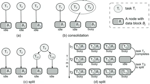
If the number of available map slots is smaller than that of map tasks in queue, one possible strategy is to consolidate map tasks so that all of them can be dispatched immediately. The data to be processed is the same no matter whether map tasks are consolidated or not. Overall overhead of map task start-up and teardown is different because there are fewer tasks after consolidation. Another potential drawback brought up by consolidation is loss of data locality. The more map tasks are consolidated, the smaller the possibility becomes that input blocks of all consolidated tasks are located on the same node. As a result, the amount of data transferred from remote nodes increases. So the optimal decision relies on the tradeoff between task overhead and data transfer cost. Plot (b) in Fig. 1 shows an example. Three map tasks , and are waiting and two nodes are available. So we can schedule two map tasks at most immediately. If we consolidate two map tasks, all map tasks can be scheduled to run immediately. In the plot, map task and are consolidated into map task which is dispatched to node where block is stored. Block is remotely accessed by task .

If the number of available map slots is larger than that of map tasks in queue, map tasks can be split to spawn new map tasks to fill idle map slots. Resultant benefits include better parallelism and load balancing. As number of map

tasks increases, overall task start-up and teardown overhead increases as well. Another disadvantage is data locality may become worse. If a map task can be dispatched to a node where its input block is stored, one of the spawned map tasks is guaranteed to be able to be dispatched to that node while others may or may not be dispatched to it depending on map slot availability. Otherwise none of its spawned map tasks after split can be dispatched to the node if they are run immediately. Plot (c) in Fig. 1 shows an example of task splitting. Initially there are four available nodes and three map tasks , and . Task is split to task . and task . and all tasks are scheduled. Task . and . share the

same input block but process different portions. Compared with the situation that splitting is not applied, task

. needs to access remotely but all nodes are utilized.

One way to mitigate the data locality problem is data replication. When there are multiple copies of a block, the possibility is larger that data-local scheduling is achievable after task spit. One extreme case is each block is replicated on all nodes so that data locality becomes less significant.

Figure 1. Task splitting and task consolidation. Arrows are scheduling decisions. Each node has one map slot and block is input of task .

B. Split Running Tasks

Besides tasks waiting in queue, running tasks can also be split dynamically to improve performance. When tasks are scheduled and running, computation time skew of tasks may slow down the progress of the whole job. Task splitting can be applied dynamically during task execution to offload some processing to other available map slots. Plot (d) in Fig. 1 shows an example. At time , four tasks are running. At time , task completes and the slot originally occupied by task becomes available while the other three tasks are still running. Task is chosen to spawn a new task . which

is scheduled to the available slot released by completed task . Again, all nodes are utilized but task . accesses

its input data remotely. C. Summary

The previous two algorithms are combined together to adjust all unfinished tasks (waiting tasks + running tasks), which achieves continuous optimization during whole lifetime of jobs.

management overhead is high and task start-up and teardown overhead is comparable to the actual execution time. We assume task execution time is significantly longer than task start-up and teardown time. If this does not hold, blocks can be enlarged to increase task granularity.

Task splitting is beneficial when loss of data locality does not impose critical performance degradation. When data are replicated on every node, the data access time is approximate no matter where a task is dispatched if data access contention (e.g. multiple tasks access different data on the same node) is not severe. If data access contention is severe, the number of map slots on each node can be tuned appropriately to achieve the optimal tradeoff between concurrency and resource use contention, so that data access does not affect scheduling much. This conclusion also holds when jobs are CPU-intensive and the data access cost is negligible. In other words, if the ratio of computation to data access is large, the computation factor is critical and other factors, such as disk I/O and network I/O, can be ignored. We focus on CPU-intensive jobs in the following discussions.

IV. SINGLE-JOB TASK SCHEDULING

First, we consider the task scheduling problem when only one job is running at most at any time. In the next section, multi-job case is discussed. The following algorithm shows how task splitting is hooked into the task scheduling process.

Algorithm skeleton

while isRunning = true: split_tasks();

schedule_tasks();

In the beginning of each scheduling iteration, task splitting is applied if needed. This step makes tradeoffs between concurrency and overhead. Then an existing task scheduling strategy (e.g. Hadoop’s data locality based scheduling) is used to schedule tasks. So task splitting can be seamlessly integrated with existing schedulers. We focus on the task splitting process and present our proposed solutions when prior knowledge about workload is known and unknown. We summarize issues shown below that need to be solved to address the problem.

a) When to trigger task splitting

b) Which tasks should be split and how many new tasks to spawn; and

c) How to split

A. Task Splitting without Prior Knowledge

When no prior knowledge is known about execution time, a strategy we term Aggressive Splitting (AS) is proposed.

1) When to trigger task splitting: The goal of task splitting is to shorten the average job turnaround time by utilizing as many nodes as possible. Assume the scheduler is invoked at time , task splitting decision is made if following inequality is satisfied

( ) + ( ) < ₍₄₎

where ( ), ( ) and are the number of map tasks in queue at time t, the number of running map tasks at

time t and the total number of map slots respectively. That means there are idle map slots even if all tasks in queue are scheduled to run immediately. In this case, the default scheduling strategy cannot use all idle slots. So the task splitting process should be initiated. Otherwise, it does not make sense to split tasks because there are no idle slots where newly spawned tasks can run. This will not make long-running tasks become stragglers because our task splitting process is invoked continuously and long-running tasks will become candidates of split target whenever there are idle slots.

2) Which tasks should be split and how many new tasks to spawn: We evenly allocate available map slots to unfinished tasks. Without prior knowledge, what we do is divide the number of idle map slots by the number of unfinished tasks to calculate how many new tasks to spawn for each task on average. Then tasks are split one by one until no map slots are idle. The algorithm skeleton is shown below.

Algorithm skeleton

UTS:set  unfinished tasks

IMS:int  number of idle map slots

MST:int  | | /

for each task T in UTS:

if IMS ≤ 0: break

if IMS < MST:

NS  split(T, IMS)

else

NS  split(T, MST)

IMS  IMS - NS

Function ( , ) splits task to spawn new tasks at most. Depending on map slot availability, split policy and overhead, the actual number of spawned tasks may be smaller than . The actual number is returned from the function call so that following code can update the number of available map slots accordingly. Implementation of split is described in next section.

3) How to split: Given a task and the maximum number of new tasks it may spawn, this section solves the problem how to split. Firstly, the number of new tasks is adjusted so that it does not exceed the number of available map slots. Data block is logically split to equally sized sub-blocks. We consider the task processing one sub-block is not splittable. So it specifies the smallest granularity of spawned tasks. For task T, the total number of sub-blocks, the number of sub-blocks that have been processed or are being processed, and the number of new tasks to spawn are denoted by

( ), ( ) and ( ) respectively. Since we don’t have prior knowledge about map execution time, we blindly spawn new tasks so that each one processes the same amount of data.

make them all complete simultaneously if map operation execution time is heterogeneous theoretically. To avoid inefficiency caused by spawning small tasks, a threshold is set to prevent small tasks being split. Optimal threshold depends on workload and map operation characteristics. It is our future work to make the threshold automatically tuned.

4) Complexity: The whole task list is scanned at most once, so time complexity is ( ) with regard to the number of tasks.

B. Task Splitting with Prior Knowledge

Now we assume that prior knowledge about task execution time is known. By prior knowledge, we mean that Estimate Remaining Execution Time (ERET) is known or predictable. ERET indicates how long a task will run before completion approximately. We propose Aggressive Split with Prior Knowledge (ASPK) to optimize job turnaround time.

1) When to trigger task splitting: The same algorithm from last section can be reused here.

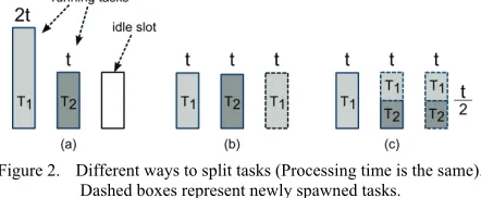
2) Which tasks should be split and how many new tasks to spawn: Ways to split tasks are not unique. Number of task splits done during whole lifetime of a job should be as small as possible without degrading performance. Fig. 2 demonstrates different ways to split tasks to achieve the same turnaround time. Graph (a) shows a scenario where there are two running tasks - , , one idle slot and no waiting tasks. ERET of and is 2 and respectively. If overhead and data locality are negligible, we definitely should split tasks to fill the idle slot. We can split task to spawn a new task and both will run for period before completion, which is demonstrated in (b). At time all tasks complete. Another way shown in (c) is to split task to spawn a new task and both will run for period /2. At time /2, two slots become idle and task is split to spawn two new tasks each of which runs for (2 /2)/3 = /2. In both cases, the final job turnaround time is t. However the number of spawned tasks is different. In (b), one task is spawned while in (c) three tasks are spawned. More task splits incur higher probability to degrade performance and destabilize system. In the example, (b) is preferred to (c).

Figure 2. Different ways to split tasks (Processing time is the same). Dashed boxes represent newly spawned tasks.

Tasks that complete last determine when a job finishes. For jobs with tasks that have highly varied execution time, the scenario should be avoided that few long tasks last much long after other short jobs complete. When long running tasks exist, to split tasks with small ERET generates smaller tasks, which doesn’t affect job turnaround time. So our

heuristics is that tasks with large ERET should be split first so that they do not become “stragglers”.

Firstly, tasks with small ERET are filtered because to split a task that will end very soon does not provide much benefit. In addition, task filtering is an optimization step that reduces the number of map tasks considered by following steps for faster processing. Secondly remaining tasks are sorted by ERET in descending order. After that, tasks are clustered into { , , … , } according to ERET so that tasks with similar ERET belong to the same cluster. Each cluster has several pieces of information including task list ( . ), the number of tasks ( . ), the sum of ERET ( . ) and the average of ERET ( . ). We go through task clusters one by one to evaluate whether task splitting is beneficial. Initially, we only consider tasks in cluster . Tasks in are split to fill all idle slots, and average task execution time is calculated. If is larger than . , it doesn’t benefit to split tasks contained in following clusters and estimated execution time of newly spawned tasks is set to . . If is significantly smaller than . , spawned tasks are small compared with tasks in . So we consider tasks from both and for split. Time is calculated and compared with . . If much smaller, we consider , and . This process is repeated until is larger than or comparable to . or all clusters are included. The algorithm skeleton is shown below.

Algorithm skeleton

IMS  number of idle map slots

UTS  unfinished tasks

FTS  filterTasks (UTS)

STS  sortByERET (FTS)

{C1,C2,…,Cm}  clusterTasks (STS)

sumERET  0, count  IMS

for cluster Ci, 1≤i≤m:

sumERET += Ci.ERET

count += Ci.Count

avgERET = sumERET / count if i = m: break

if avgERET << Ci+1.AE:

continue else

break

splitting outweighs potential gain of higher concurrency. So we filter out tasks that are close to completion without affecting overall performance. Thus the filtering process is adaptive to workloads of different types.

Clustering Task clustering algorithm is designed to group tasks with similar ERET and separate tasks with significantly different ERET. Existing clustering algorithms, such as K-means, Expectation-Maximization and agglomerative hierarchical clustering, from the machine learning community can be used without modification. Considering that scheduling routine is called frequently and its performance is critical to the whole system, we favor simple linear algorithms. Tasks being clustered have been ordered by ERET, which guarantees that tasks belonging to the same cluster are consecutive in the task list. Our current algorithm requires that the task list is scanned once by moving a “cursor” from beginning to end. A running list is maintained to contain tasks that are before the “cursor” and belong to current cluster. If ERET of the task pointed by cursor is much smaller than the average ERET of the current cluster, then the current cluster is added to cluster set and a new cluster is created which initially only contained the task pointed by cursor. This guarantees maximal ERET of tasks within a cluster is significantly smaller than average ERET of tasks within previous cluster.

3) How to split: The way to split tasks can be optimized if we also have prior knowledge about mean task execution time, network throughput, disk I/O throughput, etc. For task T, disk I/O cost, network I/O cost, and computation cost are denoted by ( ), ( ) and ( ) respectively. So total time is ( ) + ( ) + ( ), if these operations don’t overlap. Task being split is denoted by

, and newly spawned tasks are { , , …, }. Ideally, following equation should be satisfied to make tasks complete simultaneously after split.

( ) + ( ) + ( ) = ∙∙∙∙∙

= ( ) + ( ) + ( )

= ( ) + ( ) + ( )

Because we assume ( ) and ( ) are negligible compared to ( ), the above equation is converted to

( ) = ( ) = ∙∙∙ = ( ) = C ( )

So unfinished work of task T is evenly distributed to T and newly spawned tasks after split.

4) Complexity: In ASPK, complexity of sorting is

( ) and that of other operations is not greater than ( ). So overall complexity is ( ). However, sorting can be further optimized considering that in each iteration, except the first one, tasks are mostly ordered. C. Fault Tolerance

Our proposed algorithms do not handle fault tolerance directly. Task splitting is not enough to cope with situations where some tasks stall or fail due to hardware failure, severe system fluctuation or hanging process. We integrate speculative execution to solve the problem. Whenever the

system detects failure, duplicate tasks are created automatically to replace failed tasks. Now we have a complete solution which can speed single-job execution by splitting relatively long tasks and speculatively re-execute failed tasks.

V. MULTI-JOB OPTIMIZATION

We put multi-job scheduling into the context of classic queuing theory. We adopted M/G/s model [16]. Jobs arrive according to a homogeneous Poisson process. Job execution time is independent and may follow generic distributions. Also there is more than one server in the system. One difference from the classic model is that a job may use multiple servers during its execution and the execution time depends on the number of used nodes. We propose Greedy Task Splitting (GTS) which minimizes run time of each job by splitting tasks to occupy all map slots and making tasks of last round complete simultaneously. Because each job uses all available nodes, following jobs cannot execute until current running job completes. In other words, the queue time of some jobs is increased compared with non-GTS scheduling. As a result, change of job turnaround time depends on both decrease of job execution time and possible increase of job queue time. We will show that GTS gives optimal job turnaround time.

A. Optimality of Greedy Task Splitting

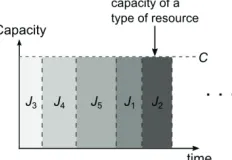
Fig. 3 shows two examples of execution arrangement of a job J. In (a), job J starts at S(J) and completes at F(J). It uses all resources during the execution. In (b), the processing is grouped to four segments - 1, 2, 3 and 4. Now we formulate the scheduling model. C denotes capacity of a certain type of resource in the system. n denotes number of jobs to run. Si (1 ≤ i ≤ n) denotes total resource requirement

of job i. Resource usage function ( , ) represents the amount of resource consumed by job i at time t. Constraints are:

≥ 0 (6)

∀ , ∑ ( , ) ≤ (7)

∀ 1 ≤ ≤ ∑ ( , ) ≥ ( ( , )dt ≥ ) (8)

and objective function is

min(∑ { ( , ) ≠ 0}) (9)

Inequality (7) means that at any moment, resource consumed by all jobs must not be more than capacity. Inequality (8) means that the sum of resource consumption by any job across time is not less than requirement of the job. The ideal case that actual resource consumption is equal to resource requirement, which means no overhead is incurred. In the objective function, { ( , ) ≠ 0} is turnaround time for job i. So our goal is to minimize overall job turnaround time.

Firstly we will show that once a job starts running, it should complete as soon as possible by using all available resources. Secondly we will convert this problem to n/1 (n jobs/1 machine) scheduling problem solved in [17].

completion time of other jobs. One fact is start time of job J does not matter when ( ) is fixed. Intuitively, all parts of execution of Job J should be placed as close to ( ) as possible. In plot (b) execution of job J is interspersed along time axis. Execution arrangement demonstrated in plot (b) can be converted to that demonstrated in plot (a) by interchanging interspersed execution segments of job J (e.g. marked by 1, 2 and 3 in the plot) and execution segments of other jobs falling into the continuous area S. After the interchange, completion time of those affected jobs either does not change or becomes earlier because their changed execution segments starts earlier. This interchange process can be iterated until each job utilizes all resources during its execution (see Fig. 3 for an example). In each iteration, only one job is considered. The whole process makes overall turnaround time monotonically decrease regardless of order of jobs picked during iterations.

Figure 3. Different ways to arrange execution of a job.

Figure 4. Multiple scheduled jobs (Each uses all resources for execution)

However, different job execution orders may result in different overall turnaround time. The next question is how to determine job execution order so that objective function is minimized. Because at any moment only one job consumes all resources, we can view the whole system as a single big virtual node. This problem becomes the n/1 problem (n jobs / 1 machine) solved in [17]. Shortest-job-first strategy gives overall optimal turnaround time. So jobs should be executed in ascending order of execution time.

B. Multi-Job Scheduling

Given a number of jobs to run, the algorithm skeleton of Shortest Job First Scheduling (SJFS) is shown below. Serial Execution Time (SET) represents how long a job runs serially.

Algorithm skeleton of SJFS

order jobs by SET in ascending order schedule jobs in turn

If we know serial execution time of all jobs that are to be run, we can apply SJFS directly. However, in real systems, it is hard, if not impossible, to know all jobs to run ahead. Jobs are submitted dynamically by end users or batch scripts. To cope with the uncertainty, we use Non Overlapped Periodic Shortest Job First Scheduling (NOPSJFS) in which SJFS is run periodically. Let I be interval that SJFS is called. So scheduling decision is made at time 0, , 2 , … Let be set of jobs that are submitted at or earlier than time t. At time ∙ , SJFS is applied to the job set ∙ ( )∙. So

jobs that are scheduled at time ∙ only include those submitted between time ( 1) ∙ and ∙ . Jobs submitted prior than time ( 1) ∙ are not considered at all even if some of them are still waiting in the queue. This strategy makes each job scheduled just once and jobs scheduled during different period do not overlap. But unexpected system fluctuation exists and prior knowledge of SET may be inaccurate. So assumptions made when a job is scheduled may be rendered useless by the time it is dispatched to run. Overlapped Shortest Job First Scheduling (OSJFS) is proposed in which all jobs are considered that have been submitted but not completed yet. To avoid starvation of long jobs, an aging factor is associated with each job which measures how long a job has been waiting in the queue. Priority is positively correlated to aging factor. So the longer a job has waited, the higher its priority becomes.

VI. EXPERIMENT

We conduct experiments using the MapReduce simulator mrsim [18] which is built on top of an event-driven framework. Table I shows the configuration of simulated system. Data is placed randomly on nodes. Each node hosts only 1 map slot. We will assess effectiveness of our approaches. So hardware configuration affects absolute job turnaround time, but it does not affect comparison between our strategies and default strategy.

TABLE I. CONFIGURATION OF TEST ENVIRONMENT

Number of nodes 64 Disk I/O - read 40MB/s Processor frequency 500MHz Disk I/O - write 20MB/s Map slots per node 1 Network 1Gbps

Two distributions are used to model execution time of map operations - Gaussian distribution and step functions abstracted from real workload trace. Firstly, we set up tests to show that our approach improves performance in single job environment.

A. Single-Job

In this set of tests, we investigate the effect of variation of map task execution time on performance. We design a micro-benchmark to measure performance improvement of task splitting. Based on total number of map slots and that of map tasks, two cases are considered.

Gaussian distribution with negative values cut off. Mean is fixed and variance is varied which is an indicator of variation of execution time of map tasks. Baseline distribution is uniform distribution with mean and coefficient of variance (CV) is zero by definition. We let Gaussian distributions have the same mean and change variance to ( ∙

) (1 ≤ ≤ 10). So CV is between 1 and 10. Job turnaround time is shown in plot (a) in Fig. 5. One observation is that job turnaround time increases as CV increases. That results from cut-off of negative values sampled from tested distributions. So the mean of sampled values is no longer and it increases slightly with CV. Both AS and ASPK improves performance significantly and performance gain increases with CV. AS incurs larger variation compared with ASPK. When CV is small, the difference between AS and ASPK is not significant. As CV becomes large, ASPK performs significantly better than AS. When CV is 10, ASPK improves AS by 50%.

Now, we increase the number of map tasks of a job to 200 to make it significantly larger than the number of map slots. Test environment is the same as previous test. Plot (b) in Fig. 5 shows results. Distributions of task execution time are the same as in previous test. Default scheduling has embedded support for load balancing. Whenever a map slot becomes available, it dispatches a waiting task to it. Because execution time of map tasks is sampled from the same distribution, the sum of task execution time for different nodes follows the same distribution as well. In other words, mixture of long and short tasks dispatched to nodes naturally makes the load balanced during early lifetime of the job. In the early phase of job execution, all map slots are occupied so that task splitting does not benefit. Towards the end of execution, all tasks are either running or completed. Any released map slot cannot be utilized because there is no waiting task. Then task splitting improves performance by rebalancing load. Considering task splitting is mostly applied near job completion, it may not benefit much. Test result shows that even in that situation, AS and ASPK improves performance by 50% at most. The larger CV is, the more efficient ASPK is compared with AS.

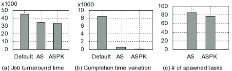
Besides synthesized workload, workload data collected in real clusters is also used. Concretely, we use cluster data published by Google [19]. It is analyzed in [20] to extract characteristics of jobs and tasks. One observation made in the paper is that task execution time for three types of jobs is bimodal. Around 75% of map tasks are short, running for approximately 5 minutes. Around 20% of map tasks are long, running for approximately 360 minutes. Execution time of the remaining 5% the map tasks is between 5 minutes and 360 minutes. This distribution is used to model task execution time in this test. Slot completion time is termed to describe when the last task run in a map slot completes. We measured both job turnaround time and the variation of slot completion time for all slots. Fig. 6 shows the results. AS and ASPK shorten job turnaround time by 20% - 30%. ASPK performs slightly better than AS by reducing job turnaround time by 5% - 10%. Standard deviation of slot completion time is shown in plot (b). For the default scheduling, the value is 8521 seconds which indicates that

the last round of map task execution results in severe load unbalancing. ASPK achieves the smallest standard deviation around 9 seconds, so that its histogram is almost invisible in the plot. This result is surprisingly good considering that the job runs for tens of thousands of seconds. For AS, standard deviation is around 570 seconds. To figure out whether the best performance of ASPK is achieved by splitting much more tasks than AS, number of spawned tasks is measured. Plot (c) shows that ASPK even has smaller number of spawn tasks than AS. So ASPK achieves shortest job turnaround time and smallest variation of slot completion time by spawning fewer tasks. This means when prior knowledge is known additional optimization done in ASPK is effective.

Figure 5. Single-Job test results (Gaussian distribution is used)

Figure 6. Single-Job test results (Real profiled distribution is used)

Above tests demonstrate that task splitting strategy improves performance significantly and the degree of improvement is related to characteristics of map tasks. B. Multiple jobs

As M/G/s model is adopted for multi-job scenario, inter-arrival time of jobs follows exponential distribution. We generate a workload to have 100 jobs each of which is synthesized according to Google cluster data. We measure average job turnaround time with and without SJF policy applied. If interarrival time is longer than job execution time, on average one job is running at most at any time. Single-Job scheduling can be used directly. So we set mean of interarrival time to be much shorter than average job execution time.

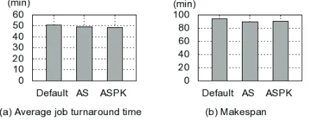
Then we tested the case where different jobs have the same serial execution time. Obviously SJF strategy does not make sense because all jobs are equally long. So we ignore SJF and evaluate task splitting strategies. Task execution time of each job follow the same distribution extracted from Google cluster data. 100 jobs are generated and all slots are used at any time except near completion. Fig. 8 shows that both job turnaround time and makespan are shortened by 5% - 10%. One well-known fact is that if a system is fully loaded, it is harder to make optimization compared with the situation where a system is partially loaded. Our test results show that even if the system is fully loaded and SJF is useless, task splitting still benefits. Considering that study in Google shows CPU utilization ratio is between 20% and 50% for their production clusters, task splitting will give more improvement in real clusters than in this test.

Figure 7. Multi-Job test results (task execution time is the same for a job)

Figure 8. Multi-Job test results (job execution time is the same)

VII. CONCLUSIONS

In this paper, we examined strategies for optimizing job turnaround time in MapReduce. Firstly, we analyzed the MapReduce model and its Hadoop implementation, and found that the way map operations are organized into tasks in Hadoop has several drawbacks, such as limit of concurrency, task completion time skew and load unbalancing. Then we proposed task splitting, which is a process to split unfinished tasks to fill idle map slots, to tackle those problems. For single-job scheduling, Aggressive Scheduling (AS) and Aggressive Scheduling with Prior Knowledge (ASPK) were proposed for cases where prior knowledge is known and unknown respectively. For multi-job scheduling, we proved that combination of Shortest-Job-First strategy and task splitting mechanism gives optimal average job turnaround time if tasks are arbitrarily splittable. Overlapped Shortest-Job-First Scheduling (OSJFS) was proposed which invokes basic short-job-first scheduling algorithm periodically and schedules all waiting jobs. We also conducted extensive

experiments to show that our proposed algorithms improve performance significantly compared with default strategy. One thing we may explore in the future is how task splitting and consolidation can benefit IO intensive applications. Tradeoffs between data access concurrency and data locality should be considered to achieve optimal performance.

ACKNOWLEDGMENT

This work is funded in part by the Pervasive Technology Institute. We would like to thank Lizhe Wang for in-depth discussions and feedbacks about our work.

REFERENCES

[1] J. Dean and S. Ghemawat, “MapReduce: simplified data processing on large clusters,” Commun. ACM 51, 1 (January 2008),p107-113 [2] X. Qiu, J. Ekanayake, S. Beason, T. Gunarathne, G. Fox, R. Barga

and D. Gannon, “Cloud Technologies for Bioinformatics Applications,” 2nd MTAGS, SC2009

[3] A. Grama, A. Gupta, G. Karypis, and V. Kumar, Introduction to Parallel Computing, 2nd edition, Pearson AddisonWesley, London, UK, 2003

[4] L. A. Barroso and U. H. Olzle, “The case for energy-proportional computing,” Computer, 40(12), 2007.

[5] W. Lu, J. Jackson, J. Ekanayake, R. S. Barga, and N. Araujo, “Performing Large Science Experiments on Azure: Pitfalls and Solutions,” in Proc. CloudCom’10, 2010, p209-217

[6] S. Kavulya, J. Tan, R. Gandhi, and P. Narasimhan, “An Analysis of Traces from a Production MapReduce Cluster,” in Proc. CCGRID '10, 2010. p. 94-103

[7] O. Sinnen, Task Scheduling for Parallel Systems, Wiley 2007 [8] M. Adler, Y. Gong, and A. L. Rosenberg. “Optimal sharing of bags of

tasks in heterogeneous clusters,” In Proc SPAA'03 2003. p1-10. [9] C. Weng and X. Lu, “Heuristic scheduling for bag-of-tasks

applications in combination with QoS in the computational grid,” FGCS, Vol. 21, no. 1, pp. 271–280, 2005.

[10] SETI@home, http://setiathome.ssl.berkeley.edu

[11] H. Casanova and F. Berman, “Parameter sweeps on the grid with APST,” in Grid Computing: making the global infrastructure a reality, F. Berman, G. Fox, and T. Hey, Eds. Wiley, 2003

[12] M. Litzkow, M. Livny, and M. W. Mutka, “Condor - A hunter of idle workstations,” In Proc. ICDCS’88 1988, pp. 104–111.

[13] BONIC http://boinc.berkeley.edu

[14] X. Zhang, Y. Qu and L. Xiao, “Improving Distributed Workload Performance by Sharing both CPU and Memory Resources,” in Proc. ICDCS’00, 2000, p.233-241

[15] V. Bharadwaj, D. Ghose, and T. G. Robertazzi, “Divisible Load Theory: A New Paradigm for Load Scheduling in Distributed Systems,” Cluster Computing Vol. 6, no. 1, Jan. 2003, p7-17 [16] D. G. Kendall, “Stochastic Processes Occurring in the Theory of

Queues and their Analysis by the Method of the Imbedded Markov Chain,” The Ann. Math Stat. Vol. 24, No. 3, Sep. 1953, pp. 338-354 [17] R. W. Conway, W. L. Maxwell, and L. W. Miller, “Theory of

Scheduling,” Addison Wesley, 1967.

[18] S. Hammoud, M. Li, Y. Liu, N. K. Alham, and Z. Liu, “MRSim: A discrete event based MapReduce simulator,” FSKD 2010, p2993-2997

[19] http://code.google.com/p/googleclusterdata/