Modelling of ship bank interaction and ship squat for ship handling simulation

(1)

Modelling of Ship-Bank Interaction and Ship

Squat for Ship-Handling Simulation

by

Jonathan Duffy, B.Eng. (Hons)

Submitted in fulfilment of the

requirements for the degree of

Doctor of Philosophy

(2)

Signed Statement

This thesis contains no material which has been accepted for a degree or diploma by the University or any other institution, except by way of background information and duly acknowledged in the thesis, and to the best of my knowledge and belief no material previously published or written by another person except where due acknowledgement is made in the text of the thesis, nor does the thesis contain any material that infringes copyright.

(3)

Authority of Access

This thesis may be made available for loan and limited copying in accordance with the Copyright Act 1968.

(4)

Abstract

This thesis reports on an investigation into the simulation of ship manoeuvring in restricted waters; in particular ship squat and ship-bank interaction.

A time-domain mathematical model has been developed to predict unsteady squat and dynamic acceleration effects for a vessel travelling in non-uniform water depth. A quasi-steady approach was adopted, where the prediction at each time step is based on steady-state heave force and pitch moment in uniform water depth. A comprehensive set of model scale experiments was conducted to investigate squat in both uniform and non-uniform water depth. Regression analysis was performed on the uniform water depth test data to develop empirical equations for steady-state squat, which were used as input to the mathematical model. The equations apply to a full form vessel and are dependent on under keel clearance parameters, channel width parameters and depth Froude number. Empirical correction factors were also developed to estimate the effect of propulsion on squat.

Good correlation was observed between predictions from the squat mathematical model and steady-state sinkage measurements for a wide range of water depth to draught ratios. Predictions from the mathematical model were also compared with unsteady sinkage measurements on a ship model travelling over a simplified ramp bank. The general trend of the predicted unsteady sinkage was reasonable, improving the realism of simulation for abrupt changes in water depth compared to predictions where acceleration effects in the vertical plane are neglected. However, the maximum unsteady sinkage was not always predicted accurately, which may be attributable to limitations and assumptions associated with the technique.

A comprehensive model scale experiment program was conducted to investigate ship-bank interaction. The following parameters were systematically varied for three different hull forms: flooded bank height, water depth, bank slope, lateral ship to bank distance, vessel speed and vessel draught. The results from these experiments were used to develop a bank parameter to estimate the effects of lateral surface piercing and flooded banks. This parameter was utilised in regression analyses to develop empirical formulae for steady-state bank induced sway force and yaw moment.

(5)

Acknowledgements

My supervisors, Dr Giles Thomas and Professor Martin Renilson, have provided a wealth of information concerning the project, along with valuable guidance and support. I would like to thank them for their enthusiasm and for always making time to answer my questions.

During the course of this work I conducted model scale experiments using the towing tank facility at the Australian Maritime College. Many thanks to towing tank staff who provided valuable assistance during the conduct of the experiments. Thanks particularly to Gregor Macfarlane and Richard Young.

Throughout this project I have worked with a number of staff and students from the Department of Maritime Engineering at the Australian Maritime College and the Department of Applied Mathematics at the University of Adelaide. In particular, I would like to thank Professor Ernie Tuck and Dr Tim Gourlay for their valuable assistance and fruitful discussions and to Roger Duffield and Gillian Carter for their assistance with model scale experiments.

I wish to thank the Australian Research Council and STN Atlas for partly funding this project.

(6)

List of Figures

Figure 0.1 Co-ordinate system xxiv

Figure 2.1 Shipflow co-ordinate system, Larsson et al. (1989) 19 Figure 2.2 Flow zones used in Shipflow, Larsson (1993) 19

Figure 2.3 Squat mathematical model flow chart 20

Figure 3.1 Schematic of simplified bank geometries for unsteady squat tests 26 Figure 3.2 Schematic of model setup for measurement of sinkage, trim and surge force 26 Figure 3.3 Schematic of model setup for measurement of heave force and

pitch moment for unsteady squat tests 27

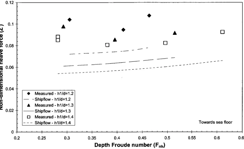
Figure 3.4 Schematic of model setup for measurement of forces and moments 28 Figure 3.5 Midship sinkage coefficient as a function of F„ h, h 1 /d=1.2, W/B=4.8 32 Figure 3.6 Midship sinkage coefficient as a function of F r,h, h 1/d=1.3, W/B=4.8 32 Figure 3.7 Midship sinkage coefficient as a function of F nh, h 1/d=1.4, W/B=4.8 33 Figure 3.8 Bow sinkage coefficient as a function of Fnh, h 1/d=1.2, W/B=4.8 33 Figure 3.9 Bow sinkage coefficient as a function of F nh, h 1/d=1.3, W/B=4.8 34 Figure 3.10 Bow sinkage coefficient as a function of F nh, h 1 /d=1.4, W/B=4.8 34 Figure 3.11 Non-dimensional heave force as a function of F nh, varying h i/d, W/B=5.0 39 Figure 3.12 Non-dimensional pitch moment as a function of F nh, varying h i/d, W/B=10.3 39 Figure 3.13 Non-dimensional pitch moment as a function of F nh, varying h i/d, W/B=3.0 40 Figure 3.14 Non-dimensional heave force (using the Bis system) as a function of F„h,

varying h i/d, W/B=5.0 40

Figure 3.15 Non-dimensional pitch moment (using the Bis system) as a function of F„h,

varying h i/d, W/B=10.3 41

Figure 3.16 Non-dimensional heave force as a function of F ni„ varying W/B, h 1/d=1.2 41 Figure 3.17 Non-dimensional pitch moment as a function of F nh, varying W/B, 12 1 /(1=1.7 42 Figure 3.18 Centre of pressure location as a function of F ni„ varying W/B, h 1/d=1.7 42 Figure 3.19 Predicted sinkage at forward perpendicular as a function of F nn,

varying W/B, h 1/d=1.7 43

(12)

Figure 3.26 Schematic of additional heave force due to propulsion 50 Figure 3.27 Additional heave force due to propulsion as a function of F nh, varying T",

h 1/d=1.1 50

Figure 3.28 Additional pitch moment due to propulsion as a function of Fth, varying T",

h1/d=1.1 51

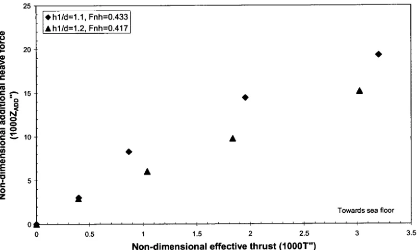
Figure 3.29 Additional heave force due to propulsion as a function of h i/d,

varying T" and Fri', 51

Figure 3.30 Additional pitch moment due to propulsion as a function of h i/d,

varying T" and FnL 52

Figure 3.31 Longitudinal position of additional heave force due to propulsion as a function of

Fnh, varying T", h1/d=1.1 52

Figure 3.32 Longitudinal position of additional heave force due to propulsion as a function of

Fni„ varying T", h 1/d=1.2 53

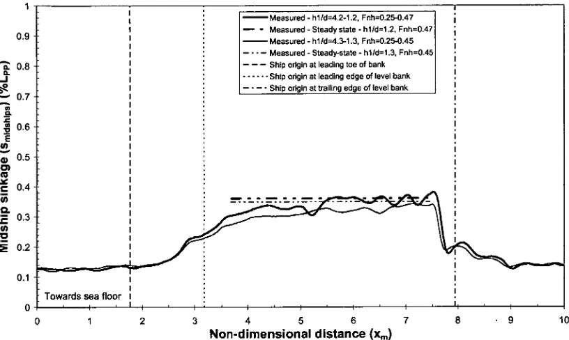
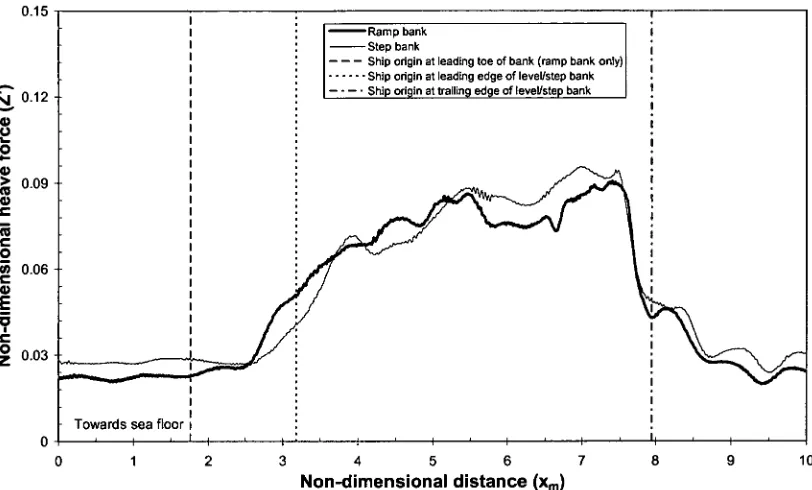
Figure 3.33 Sinkage over ramp bank, F=0.30-0.55, h 1/d=4.3-1.3 57 Figure 3.34 Trim over ramp bank, Fnh=0.30-0.55, h 1/d=4.3-1.3 57 Figure 3.35 Midship sinkage over ramp bank for different water depths 58 Figure 3.36 Bow sinkage over ramp bank for different water depths 58 Figure 3.37 Midship sinkage over ramp bank for different vessel speeds 59 Figure 3.38 Bow sinkage over ramp bank for different vessel speeds 59 Figure 3.39 Heave force over ramp bank and step bank, h 11d=4.3-1.3, Fnh=0.35-0.63 60 Figure 3.40 Pitch moment over ramp bank and step bank, h i/d=4.3-1.3, Fnh=0.35-0.63 60 Figure 3.41 Comparison between measured heave force and Shipflow predictions,

W/B=10.3 62

Figure 3.42 Comparison between measured pitch moment and Shipflow predictions,

W/B=10.3 62

Figure 4.1 Non-dimensional additional heave force due to propulsion as a function of

T",varying h i/d 73

Figure 4.2 Non-dimensional additional pitch moment due to propulsion as a function of

T",varying h i/d 73

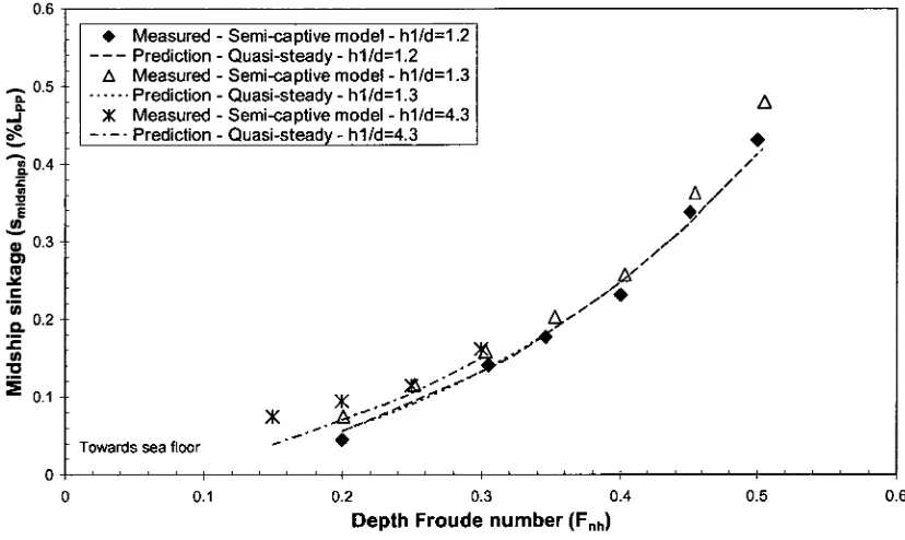
Figure 4.3 Comparison of midship sinkage measured from semi-captive experiments and

quasi-steady mathematical model predictions 76

Figure 4.4 Comparison of bow sinkage measured from semi-captive experiments and

quasi-steady mathematical model predictions 76

(13)

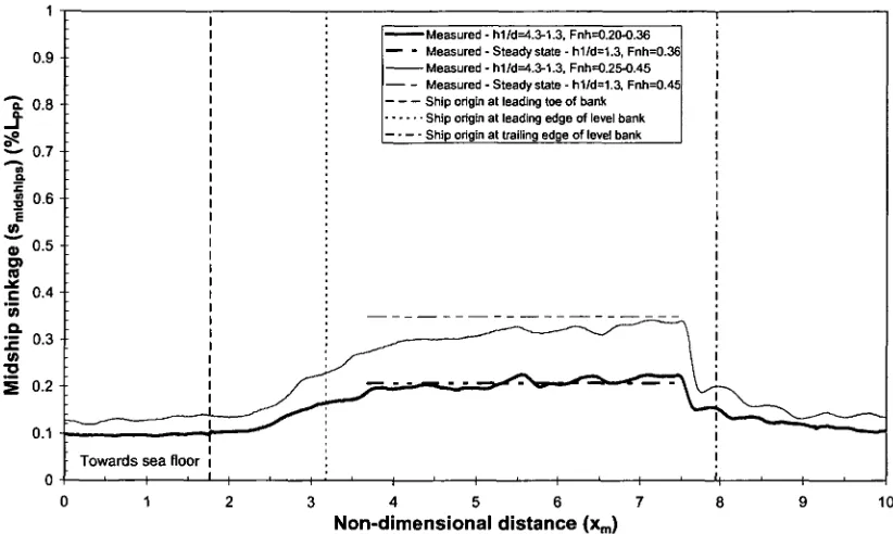
Figure 4.9 Midship sinkage over ramp bank, F6=0.25-0.43, h1/d=4.51-1.51 79 Figure 4.10 Bow sinkage over ramp bank, F6=0.25-0.43, h1/d=4.51-1.51 79 Figure 4.11 Midship sinkage over ramp bank, F6=0.20-0.36, hi/d=4.3-1.3 80 Figure 4.12 Bow sinkage over ramp bank, F6=0.20-0.36, h1/d=4.3-1.3 80 Figure 4.13 Midship sinkage over ramp bank, F6=0.25-0.45, h1/d=4.3-1.3 81 Figure 4.14 Bow sinkage over ramp bank, F6=0.25-0.45, h1/d=4.3-1.3 81 Figure 4.15 Midship sinkage over ramp bank, F6=0.30-0.55, h1/d=4.3-1.3 82 Figure 4.16 Bow sinkage over ramp bank, F6=0.30-0.55, h1/d=4.3-1.3 82 Figure 4.17 Midship sinkage over ramp bank, F6=0.25-0.47, h1/d=4.2-1.2 83 Figure 4.18 Bow sinkage over ramp bank, F6=0.25-0.47, h1/d=4.2-1.2 83 Figure 5.1 Schematic of model set up for sway force and yaw moment tests 88

Figure 5.2 Parameters defining bank geometry 90

Figure 5.3 Non-dimensional sway force as a function of Fnh, MarAd L series model 92 Figure 5.4 Non-dimensional yaw moment as a function of Fnh, MarAd L series model 92 Figure 5.5 Non-dimensional sway force as a function of Fnh 93 Figure 5.6 Non-dimensional yaw moment as a function of Frill 93

Figure 5.7 Non-dimensional sway force as a function of Fth, MarAd L series model 94 Figure 5.8 Non-dimensional yaw moment as a function of Fnh, MarAd L series model 94 Figure 5.9 Non-dimensional sway force as a function of d/(hi-d) 96 Figure 5.10 Non-dimensional yaw moment as a function of d/(hi-d) 96 Figure 5.11 Non-dimensional sway force as a function of yB, for surface piercing banks 98 Figure 5.12 Non-dimensional yaw moment as a function of yBt for surface piercing banks 98 Figure 5.13 Non-dimensional sway force as a function of yBt for flooded banks,

MarAd L series model 99

Figure 5.14 Non-dimensional yaw moment as a function of yBt for flooded banks,

MarAd L series model 99

Figure 5.15 Non-dimensional sway force as a function of 102p/h1) 101 Figure 5.16 Non-dimensional yaw moment as a function of 1-(h2cih1) 101 Figure 5.17 Non-dimensional sway force as a function of 1-(h2p/121) 102 Figure 5.18 Non-dimensional yaw moment as a function of 1-(h2p/h1) 102 Figure 5.19 Non-dimensional sway force as a function of F„L, varying ap, d/(h1 d)=3.35,

Ypt/B=1.00, 1-(h21/h1)=1.00, MarAd L series model 104

(14)

Figure 5.21 Non-dimensional sway force as a function of ap 105

Figure 5.22 Non-dimensional yaw moment as a function of up 105

Figure 5.23 Non-dimensional sway force as a function of F ni„ ypt/W=0.162, d/(h1-d)=9.63,

1-(h21,/h1)=1.00, ap=90° 107

Figure 5.24 Non-dimensional yaw moment as a function of Fnh, ypt/W=0.162, d/(h1-d)=9.63,

1-(h21,/h1)=1.00, ap=90° 107

Figure 5.25 Non-dimensional sway force as a function of Fnh for bulk carrier and

containership models 108

Figure 5.26 Non-dimensional yaw moment as a function of Fnh for bulk carrier and

containership models 108

Figure 5.27 Non-dimensional sway force as a function of Fnii for bulk carrier and containership

models, ypt/W=0.118, d/(h 1 -d)=5.13, 1-(h2p/h1)=1.00, ap=90° 109

Figure 5.28 Non-dimensional yaw moment as a function of Fnh for bulk carrier and

containership models, ypt/W=0.118, d/(h1-d)=5.13, 1-(h2p/h1)=1.00, ap=90° 109

Figure 5.29 Comparison between measured sway force and Shipflow predictions, yBt=-0.403,

1-(h2p/h1)=-1, 1 -(h21111)=1 , a=90°, MarAd L series model 113

Figure 5.30 Comparison between measured yaw moment and Shipflow predictions, yBt=-0•403,

1-(h2 /h1)=1, 1-(h2s1h1)=1, ap=90°, MarAd L series model 113

Figure 6.1 Non-dimensional sway force as a function of d/(h i-d) 118

Figure 6.2 Non-dimensional yaw moment as a function of d/(hi-d) 118

Figure 6.3 Lateral ship to bank distances for surface piercing banks, Ch'ng (1991) 124 Figure 6.4 Lateral ship to bank distances for flooded and surface piercing banks 125 Figure 6.5 Non-dimensional sway force as a function of yBt, varying up,

d/(h1-d)=9.63, MarAd L series 125

Figure 6.6 Non-dimensional sway force as a function of yB5, varying up,

Figure 6.9 Non-dimensional yaw moment as a function of yBt, varying ap,

Figure 6.10 Non-dimensional yaw moment as a function of yB5, varying ap,

Figure 6.11 Non-dimensional yaw moment as a function of yB6, varying ap,

Figure 6.12 Non-dimensional yaw moment as a function of yB7, varying up,

(15)

Figure 6.14 cn as a function of Fith, MarAd L series model 132

Figure 6.15 c3, as a function of d/(hi-d) 133

Figure 6.16 c. as a function of d/(hi-d) 133

Figure 6.17 Non-dimensional sway force as a function of 1-(h2p/h1), MarAd L series model 134

Figure 6.18 Non-dimensional yaw moment as a function of 1-(h2p/h1), MarAd L series

model 134

Figure 6.19 Non-dimensional sway force as a function of BPy6 for varying bank submergence,

Ypt/B=0.69, MarAd L series 135

Figure 6.20 Non-dimensional yaw moment as a function of BPN6 for varying bank submergence,

ypt/B=0.69, MarAd L series 135

Figure 6.21 Non-linear relationship between non-dimensional sway force and yaw moment with

CB, d/(h1-d)=9.63, ypt/W=0.097, 1-(h2p/h1)=1.00, ap=90°, MarAd L series, MarAd F

series, 5-175 containership 138 Figure 6.22 Sample of a test conducted to assess the accuracy of regression equations,

y,/B=1.00, Yst/13=5 .15, d/(h 1 -d)=2.00, 1-(h2p/h1)=0.47, 1-(h2,/h1)=1.00, ap=90°,

MarAd L 140

Figure 6.23 Comparison between regression prediction and non-dimensional sway force

measured by Dand (1981), Cases 1 - 4 144

Figure 6.24 Comparison between regression prediction and non-dimensional sway force

measured by Dand (1981), Cases 5 -8 144

Figure 6.25 Comparison between regression prediction and non-dimensional yaw moment

measured by Dand (1981), Cases 1 —4 145

Figure 6.26 Comparison between regression prediction and non-dimensional yaw moment

measured by Dand (1981), Cases 5 — 8 145

Figure 6.27 Predicted ship path using empirical equations from the present study in the AMC

ship-handling simulator for the Port of Weipa 147

Figure 6.28 Predicted bank induced sway force and yaw moment for the simulation of a

manoeuvre at the Port of Weipa (output from AMC ship-handling simulator) 148 Figure B1 Body plan of MarAd L series model (Roseman 1987) 162 Figure B2 Body plan of MarAd F series model (Roseman 1987) 162

Figure B3 Body plan of S-175 containership (ITTC 1987) 163

Figure B4 MarAd L series model with propeller fitted 163

Figure Cl Channel walls constructed in towing tank for squat tests 164 Figure C2 Photograph showing steel port wall set up in the towing tank 165

Figure C3 Flooded bank assembly prior to water fill 166

Figure El Non-dimensional sway force as a function of FnL, yBt=-0.629, d/(h1-d)=5.13,

(16)

Figure E2 Non-dimensional yaw moment as a function of FnL, ym=-0.629, d/(h1-d)=5.13,

1-(h21fli1)=1.00, 1-(h2s/h1)=1.00, a=90°, as=90°, MarAd L 174 Figure E3 Non-dimensional sway force as a function of FnL, ym=-0.629, d/(h1-d)=2.00,

1-(h2p/h1)=1.00, 1-(h2s/h1)=1.00, a=90°, as=90°, MarAd L 175 Figure E4 Non-dimensional yaw moment as a function of Fnu Ys -O.629, d/(h1-d)=2.00,

(17)

List of Tables

Table 2.1 Number of panels for a Shipflow mesh, W/B=3, h 1/d=1.4 18

Table 3.1 Principal particulars of models 25

Table 3.2 Test program: effect of scale on squat measurement using MarAd F series 30 Table 3.3 Test program: effect of vessel speed, water depth and channel width on heave force

and pitch moment due to squat, B/d=4.42 36

Table 3.4 Test program: effect of vessel speed, water depth and vessel draught on heave force

and pitch moment due to squat, W/B=10.3 36

Table 3.5 Test program to investigate the influence of propulsion on squat 46

Table 3.6 Test program for unsteady squat tests 54

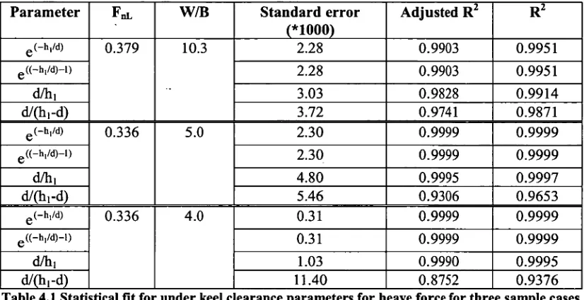
Table 4.1 Statistical fit for under keel clearance parameters for heave force for three sample

cases 66

Table 4.2 Statistical fit for under keel clearance parameters for pitch moment for three sample

cases 66

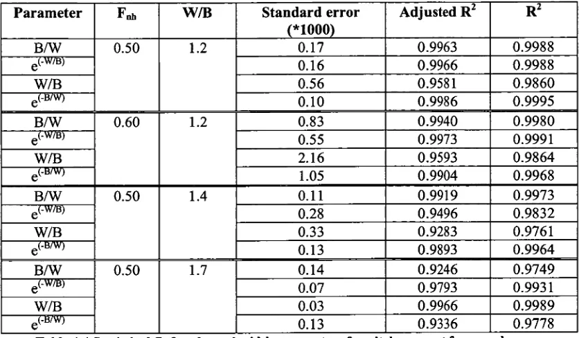
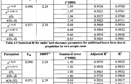
Table 4.3 Statistical fit for channel width parameters for heave force for sample cases 67 Table 4.4 Statistical fit for channel width parameters for pitch moment for sample cases 68 Table 4.5 Statistical fit for under keel clearance parameters for additional heave force due to

propulsion for two sample cases 71

Table 4.6 Statistical fit for under keel clearance parameters for additional pitch moment due to

propulsion for two sample cases 71

Table 6.1 Statistical fit for under keel clearance parameters for sway force for three sample

cases 119

Table 6.2 Statistical fit for under keel clearance parameters for yaw moment for three sample

cases 119

Table 6.3 Statistical fit for ship to bank distance parameters for a sample of surface piercing

bank cases for sway force 121

Table 6.4 Statistical fit for ship to bank distance parameters for a sample of surface piercing

bank cases for yaw moment 121

Table 6.5 Statistical fit for ship to bank distance parameters for a sample of flooded bank

cases for sway force 122

Table 6.6 Statistical fit for ship to bank distance parameters for a sample of flooded bank

cases for yaw moment 123

Table 6.7 Analysis of hull form parameters for non-dimensional sway force, Fnh=0.176, 0.194, 0.219, ci/(11 1-d)=9.63, ypt/W=0.097, 1-(h211h1 )=1.00, a90, MarAd L series,

(18)

Table 6.8 Analysis of hull form parameters for non-dimensional yaw moment, FO. 176, 0.194, 0.219, cl/(h1-d)=9.63, ypt/W=0.097, 1-(h21,/h1)=1.00, u=90°, MarAd L series,

MarAd F series, S-175 containership 137

Table 6.9 Analysis of hull form parameters for non-dimensional sway force, Fith=0.269,

0.296, d/(h1-d)=9.63, 1-(h2p/h1)=0.65, ypt/W=0.097, ap=90°, MarAd L series,

Table 6.10 Analysis of hull form parameters for non-dimensional yaw moment, Fnh=0.269,

0.296, 0.219, d/(h1-d)=9.63, ypt/W=0.097, 1-(h2p/h1)=0.65, ap=90°, MarAd L series,

(19)

Nomenclature

A Panel area Vessel beam CB Block coefficient Cp Pressure coefficient

Vessel draught

DB Bank height

Fnh Depth Froude number,

gh

JgL p

Acceleration due to gravity Water depth in channel h2p Depth of water over port bank h2s Depth of water over starboard bank In Pitch mass moment of inertia Edyy Added pitch mass moment of inertia Izz Yaw mass moment of inertia

L pp Length between perpendiculars

Pitch moment due to squat M' Non-dimensional pitch moment_'

— pU 2 L pp 3

2 Length Froude number,

MADD MADD"

Mdaroping

Mhydrostatic

Mpropelled

Munpropelled

Nr, Non-dimensional pitch moment,

pgYolapp

Additional pitch moment due to propulsion

ADD Non-dimensional additional pitch moment due to propulsion,

Damping pitch moment Hydrostatic pitch moment Pitch moment on propelled hull Pitch moment on unpropelled hull

(20)

Outward normal Yaw moment

N' Non-dimensional yaw moment,

pu2Lpp2d

2 N" Non-dimensional yaw moment,

pgVoLpp

Pressure

Free stream pressure

Pd Dynamic pressure

R2 Coefficient of determination

R2adjusted Adjusted coefficient of determination

Show Bow sinkage (at forward perpendicular)

smidsbips Midship sinkage

sstem Stern sinkage (at aft perpendicular) Ss Ship cross-sectional area

scbow Bow sinkage coefficient scmidships Midship sinkage coefficient SS Sum of squares

So Channel cross sectional area Time

propelled — Xtutpropolled)

Effective thrust (X

T" Non-dimensional effective thrust,

Velocity Velocity vector Free stream velocity U. Free stream velocity vector

Component of U along x ship body axis Component of U along y ship body axis Velocity along y ship body axis

Channel width

(21)

X

Xpropelled Xunpropelled XADD XLCF-FP

Surge force

Surge force on propelled hull Surge force on unpropelled hull

Longitudinal position of additional heave force due to propulsion Distance from static LCF to forward perpendicular

Non-dimensional distance along channel centreline (x*/Lpp) Distance along channel centreline relative to an earth fixed point Distance from midships to static LCF

Sway force

Non-dimensional sway force,

1 pU 2 Lppd 2

ylf

YBt

Non-dimensional force,

B sway

pgV o

Ship to bank distance parameter, (

1 Y_pty_st 2

YBi Ship to bank distance parameter, [ — + —1 1 — B

pt si

YPi Distance from ship's centreline to port bank on different vertical planes

Ypw Width of port flooded bank

Ypt Distance from ship's centreline to toe of bank on port side

Ysi Distance from ship's centreline to starboard bank on different vertical planes

Yst jcp

Distance from ship's centreline to toe of starboard bank Sinkage at LCF

ZLCF0 Sinkage at LCF (initial condition) Z LCF Heave velocity at LCF

Z LCFO Heave velocity at LCF (initial condition) Z LCF Heave acceleration at LCF

ZFp Sinkage at forward perpendicular due to pitch

(22)

Heave force due to squat

Z' Non-dimensional heave force due to squat,

Z" Non-dimensional heave force, Pgv. ZADD Additional heave force due to propulsion

—1 pU 2 L pp 2

2

Z

ZADD" Non-dimensional additional heave force due to propulsion, ADD Pg\70

Zdampmg Damping heave force Zhydrostatic Hydrostatic heave force Zpropelled Heave force on propelled hull Zunpropelled Heave force on unpropelled hull

Water density

Volumetric displacement at rest V Del operator

u

p

Port bank angle with respect to the horizontal plane as Starboard bank angle with respect to the horizontal plane a Source strength

A Ship displacement SA Heave added mass 0 Pitch

O Pitch velocity

60 Pitch velocity (initial condition) 0 Pitch acceleration

4:13, Velocity potential

(Do Double body velocity potential

11 Free surface elevation

Double body free surface elevation 'Nave Heave damping coefficient

ipitch Pitch damping coefficient

(23)

Yaw velocity Yaw acceleration

Abbreviations

AMC Australian Maritime College AP Aft perpendicular

FP Forward perpendicular

ITTC International Towing Tank Conference LCB Longitudinal centre of buoyancy LCF Longitudinal centre of floatation LVDT Linear variable differential transformer MCTC Moment to change trim one centimetre NTSB National Transportation Safety Board

PIANC Permanent International Association of Navigation Congresses TPC Tonnes per centimetre

(24)

Co-ordinate System

The co-ordinate system used in the present study is shown in Figure 0.1, unless stated otherwise. The origin is situated at midships on the static waterline.

(25)

Chapter 1 Introduction

1.1 Background

A ship operating within a port environment is likely to travel in close proximity to waterway boundaries. The change in flow due to interaction with these restrictions influences the manoeuvring behaviour of a ship. These interactions are exacerbated by the fact that ship size is steadily increasing to cope with productivity demands. Real-time simulation of ship manoeuvring is widely used to predict the path of a ship within restricted water to assist with tasks such as channel design, developing safe port operating procedures and conducting ship operation training. This thesis reports on a study into the modelling of the interaction between a ship and waterway boundaries, i.e. the sea floor and lateral banks.

(26)

square of the ship speed in the sub-critical flow regime (Norrbin 1978). The attraction sway force can also be described, in general, as a simple Bernoulli effect due to the flow contraction between the ship and near bank. The sway force generally changes to repulsion from the near bank when the blockage is increased and/or when the vessel speed is sufficiently high. The bank induced sway force and yaw moment can influence the manoeuvring properties of a ship, which may lead to potentially dangerous situations, such as collisions with other ships or with waterway boundaries.

Accurate prediction of squat and ship-bank interaction is crucial for realistic real-time simulation of the manoeuvring behaviour of a ship in restricted water. If squat can be predicted accurately, ship-handling simulators may be used to determine the optimum under keel clearance so that the payload can be maximised whilst minimising the risk of grounding. Accurate prediction of ship-bank interaction will enable simulators to be used to determine optimum channel widths and/or to determine if vessels can safely manoeuvre within proposed or existing channel geometries. Such predictions will allow accurate assessment of dredging requirements, potentially reducing dredging expenses. Also, safe operating ship speeds can be determined for specific operating conditions in relation to squat and ship-bank interaction. Numerous prediction techniques exist to predict squat in uniform depth. In comparison, the prediction of squat in non-uniform depth has received little attention to date (Gourlay 2003). Previous predictions of squat in non-uniform depth have generally been undertaken using constant depth formulae based on the average depth under the ship, assuming that the ship speed and water depth are both sufficiently slowly varying functions of time to neglect unsteadiness NTSB (1993). It is uncertain whether this approach will under or over predict unsteady squat. Hatch (1996) developed a mathematical model to predict unsteady squat, but poor correlation was observed with model scale measurements.

In recent years a number of studies have been conducted to predict the interaction between ships and lateral surface piercing banks for the purpose of ship-handling simulation, for example Ch'ng et al. (1993) and Vantorre (1995). However, experimental data and prediction methods for the interaction between ships and flooded banks for ship-handling simulation are scarce, limiting the applicability of most simulators to surface piercing bank cases.

1.2 Objectives

As identified in Section 1.1, there is a need for a practical prediction technique for unsteady squat including dynamic acceleration effects and for the quantification of interaction between a ship and flooded lateral banks.

Therefore, the objectives of this work are:

• to develop and validate a practical technique for predicting vessel motion in the vertical plane due to unsteady squat for use in real-time ship-handling simulators, and

(27)

1.3 Methodology

The simulation of both squat and ship-bank interaction was undertaken in two steps; the first was the prediction of steady-state forces and moments in the horizontal and vertical planes, and the second was the prediction of real-time motions using quasi-steady mathematical models. The requirement was to develop techniques to predict steady-state squat and ship-bank interaction in real-time simulation, whilst achieving sufficient accuracy. Developing empirical formulae by performing regression analysis on model scale measurements is an effective method to accurately account for the complex restricted water flow phenomena, whilst satisfying the real-time computation condition. Therefore, model scale experiments were conducted to measure steady-state forces in the horizontal and vertical planes on different ship models for a wide range of channel geometries and waterway parameters. The number of model scale experiments that could be conducted was limited by the resources and time required to perform them. Steady-state heave force and pitch moment due to squat and bank induced sway force and yaw moment were also predicted using a three-dimensional panel method. The aim was to compare the predictions to model scale experiment results to assess if the method was sufficiently accurate to be used to extend the steady-state experimental data matrix for the regression analysis.

Using regression analysis techniques empirical formulae were developed for steady-state heave force and pitch moment due to squat for an unpropelled bulk carrier hull form and a correction was generated for the effect of propulsion. The ship-bank interaction experiments were used to develop a bank parameter to allow approximation of the effects of lateral surface piercing and flooded banks. This parameter was utilised in regression analyses to develop the empirical formulae for steady-state bank induced sway force and yaw moment.

A mathematical model was developed to predict squat and associated acceleration effects for a vessel travelling in water of non-uniform depth. The empirical formulae to predict steady-state heave force and pitch moment due to squat were used as input to the real-time, two degree of freedom mathematical model. Predictions from the quasi-steady model were assessed against model scale steady-state sinkage measurements and unsteady sinkage measurements on a vessel travelling over a simplified ramp bank.

The empirical formulae to predict steady-state bank induced sway force and yaw moment were validated against independent model scale measurements from literature. The formulae were incorporated into an existing mathematical model to predict vessel motions in the horizontal plane. The quasi-steady technique was used to predict the path of a vessel for a manoeuvre where ship-bank interaction is used to aid a turn and the predicted path was compared to that known to occur in the real-life manoeuvre.

The novel components of the work and contributions to knowledge in the field of ship-handling simulation include:

• A comprehensive set of model scale experiments has been conducted for a wide range of conditions, enhancing the understanding of vessel squat and ship-bank interaction. • Empirical equations have been developed to predict the steady-state heave force and

(28)

and channel widths. Correction factors for the influence of propulsion have also been presented.

• A mathematical model has been developed to estimate unsteady squat and dynamic acceleration effects in the vertical plane, which is applicable to a wide range of bathymetries.

• Empirical formulae have been developed through the use of a bank parameter that enables estimation of the influence of port and starboard surface piercing and flooded banks. With the capability to predict the influence of flooded banks for such a wide range of cases the proposed prediction technique is applicable to a broader range of port geometries, when compared to previous prediction techniques.

• The empirical formulae to predict steady-state ship-bank interaction have been incorporated into an existing mathematical model to predict the real-time manoeuvring behaviour of a ship travelling in close proximity to lateral flooded and surface piercing banks.

1.4 Overview of thesis structure

A review of previous work on the prediction of squat and ship-bank interaction is given in Chapter 2, together with mathematical details concerning the prediction techniques used in the present study.

Chapters 3 and 4 relate exclusively to ship squat. Both steady and unsteady model scale experimental results are presented and discussed in Chapter 3, whilst in Chapter 4 empirical equations are developed to predict steady-state heave force and pitch moment in the squat mathematical model. Unsteady squat predictions using the mathematical model are compared with unsteady squat measurements from model scale experiments in Chapter 4.

Ship-bank interaction is addressed in Chapters 5 and 6. Model scale experiment results for bank induced sway force and yaw moment are presented in Chapter 5. In Chapter 6 empirical equations are developed to predict steady-state bank induced sway force and yaw moment and are validated against independent results from literature. These equations are incorporated into an existing mathematical model to predict the path of a ship for a manoeuvre that is performed in an Australian port, where bank effect is utilised to aid a turn. The predictions are compared to the ship path that is known to occur in the real-life manoeuvre.

Finally, conclusions and recommendations for further work for both squat and ship-bank interaction are presented in Chapter 7.

(29)

Chapter 2 Squat and Ship-Bank Interaction Prediction

Techniques

2.1 Introduction

Existing prediction techniques for ship squat and ship-bank interaction are reviewed in Section 2.2.

The aim of the present study was to develop real-time simulation models for ship squat and ship-bank interaction. Due to the complex flow phenomena associated with vessel transit in restricted water the proposed methodology for real-time simulation was to use regression analysis techniques to develop empirical equations to predict steady-state forces and moments for use as input to quasi-steady mathematical models. However, predictions were also performed for steady-state cases using a three-dimensional panel method with the aim to determine if the method is sufficiently accurate to complement experimental measurements for input data to the regression analyses. In Section 2.3 background on the three-dimensional panel method is given along with details concerning the regression techniques used to develop the empirical equations.

A quasi-steady mathematical model has been developed to predict unsteady squat and associated acceleration effects in the vertical plane. An existing mathematical model was used to predict sway and yaw motions due to ship-bank interaction. Both models are outlined in Section 2.4.

2.2 Background

2.2.1 Steady-state prediction

A steady-state case is defined as a ship moving at constant speed in water of uniform depth, travelling parallel to straight uniform lateral banks.

Squat

Numerous techniques exist to predict steady-state vessel squat. These can be broadly classified into the following categories: prediction of water level depression, theoretically based prediction of sinkage and trim, semi-empirical prediction of sinkage and trim, and empirically based prediction of sinkage and trim.

(30)

depression is assumed to be equal to the ship sinkage, ignoring the trim of the vessel. This approach assumes that the flow is one-dimensional and the velocities of the water particles in any channel cross section are constant over that cross section. This technique is useful near the ship where the lengthwise-averaged water-level depression and ship's sinkage are similar. However, this assumption breaks down as the channel width becomes large with respect to the vessel beam.

The prediction of water level depression and back flow velocity using the momentum approach was undertaken by Sharp and Fenton (1968) and Bouwmeester (1977). The latter author accounted for the water level rise in front of the bow and made use of an empirical correction factor to improve the accuracy of the technique. Blaauw and Van Der Knaap (1983) compared predictions from the Bouwmeester method against model scale experiment sinkage results. The correlation was reasonable for channel width to vessel beam ratios between 5 and 8. They found that sinkage predictions from Sharp and Fenton's method were around 20% less than those of Bouwmeester.

Ship sinkage has been predicted by the water level depression technique using the continuity equation in conjunction with the conservation of energy by many authors, such as Balanin and Bykov (1965), Constantine (1961), Tothill (1967), McNown (1976) and Gates and Herbich (1977). These methods all yielded similar results, which showed reasonable correlation with measured sinkage values for channel width to vessel beam ratios less than 5. Vessel sinkage was under predicted using this prediction technique for greater channel width to beam ratios (Blaauw and Van Der Knaap 1983).

Tuck (1966) used slender body theory to predict vertical forces on slender ships in shallow water at both sub-critical and super-critical speeds, sinkage and trim were then calculated using ship hydrostatic particulars. The predictions showed reasonable correlation with scale model experiment results presented by Graff et al. (1964) for low water depth to ship length ratios and low depth Froude numbers. However, the correlation deteriorated for larger water depths and as the depth Froude number approached 1.0. Blaauw and Van Der Knaap (1983) found that Tuck's theory gave reasonable agreement with experimental results for channel width to vessel beam ratios between 6 and 13. It was found that trim correlated reasonably well with model experiment results, except for some cases with an LNG carrier model, where the wrong trim direction was predicted. Hooft (1974) proposed a modified version of Tuck's formula to compute bow squat and Huuska (1976) proposed new coefficients, for Hooft's formulae, and introduced a blockage correction factor. Vermeer (1977) proposed approximations to the coefficients in Tuck's formulae to predict sinkage and trim for ships in narrow canals. Tuck (1967) extended his earlier work to account for the presence of vertical side walls, but only for sub-critical flow, with the assumption that the channel width is comparable with the ship length. The work was extended further by Tuck and Taylor (1970) to a three-dimensional squat theory for water of finite depth and width. Slender body theory was further utilised to predict squat for the case of a ship travelling in a dredged channel (Beck et al. 1975).

(31)

Rubin (1984) used a two-dimensional theory to predict steady-state squat in shallow water based on non-linear directed sheet theory. Good agreement was found with data from Graff et al. (1964) for ship length to water depth ratios of 3 and 4.8, but poorer correlation was observed

when the ship length to water depth ratio was increased to 8. Kijima and Higashi (1996) presented a prediction method for ship squat considering non-linear terms on the effect of the free surface using slender body theory. The results of the numerical calculation on sinkage agreed well with model experiment results but showed an over estimation of trim. A simpler prediction method based on principal ship particulars was also presented by Kijima and Higashi (1996). The predictions using this simple prediction were reasonable when compared to model experiment results; however, it was concluded that further work is required to include the influence of a working propeller. Gourlay (2000) applied slender body theory to predict squat in open water of finite depth.

Semi-empirical techniques have been used to predict squat, where empirical correction factors were used in conjunction with numerical methods, for example Dand and Ferguson (1973), Fuehrer and Romisch (1977) and Anlcudinov and Jakobsen (1996). Dand and Ferguson (1973) and Fuehrer and Romisch (1977) developed empirical correction factors to be used in conjunction with a one-dimensional theory based on the continuity equation and conservation of energy. Dand and Ferguson (1973) made use of an effective width parameter developed by Tuck (1967) and also developed propulsion correction factors. They obtained full-scale measurements from a number of ships and compared the results to their predictions. The comparisons were encouraging given the practical limitations of the accuracy of the full-scale results. Blaauw and Van Der Knaap (1983) compared the predictions from Dand and Ferguson and Fuehrer and Romisch with measured squat values. They found that the predictions using the method proposed by Dand and Ferguson showed reasonable correlation with model experiment results for channel width to vessel beam ratios between 7 and 13. The predictions were found to underestimate squat for channel width to beam ratios less than 7. The Fuehrer and Romisch approach was found to generally over predict squat. However, Millward (1990), on comparing Fuerhrer and Romisch's prediction to model scale experiments found that it underestimated bow squat by up to 50%, but was more accurate for midship sinkage.

(32)

Model scale experiments have also been used to develop empirical equations for ship squat in laterally restricted water. For example, Blaauw and Van Der Knaap (1983) conducted experiments in a flume tank with self-propelled scale models of a VLCC and an LNG carrier for a number of different channel widths and water depths. They measured the water-level depression near the model and near the lateral bank, and developed an empirical equation to describe the relationship between the water-level depression at the ship and the lateral bank. Barrass (1979), Millward (1992), and Eryuzlu et al. (1994) developed empirical formulae to predict squat in laterally restricted water of finite depth.

Collinson (1994) compared the results from well known published sinkage and trim prediction techniques against experimental results from Millward (1990, 1992) and found that the predictions produced a large divergence of results and that no single prediction technique provided the best correlation for all cases. He stated that no single method accurately predicted squat for all ships and conditions. Dand (1996) compared squat prediction methods for typical ships. It was found that there was a wide scatter in the results, although there was some evidence of 'common ground' near the centre of the scatter.

Ship-bank interaction

There have been a number of simplified bank effect prediction techniques developed based upon model scale investigations. For example, Schoenherr (1960) used model scale experiment results to develop design charts, from which bank induced sway force and yaw moment could be determined for a range of channel parameters. Fuehrer and Romisch (1983) conducted a comprehensive set of model scale experiments on models fitted with propellers and rudders. An empirical equation for the prediction of rudder force was developed along with a series of diagrams for calculating lateral forces and yaw moment acting on a ship for different channel widths at various drift angles. The diagrams were based on the equilibrium of lateral hydrodynamic forces acting on a ship and can be used to determine optimum channel profiles. The predictions were found to correlate well with experiment results published by Gates and Herbich (1977).

Several empirical equations have been developed to predict bank induced sway force and yaw moment utilising linear superposition of the effect of port and starboard banks. Norrbin (1985) presented empirical equations to predict bank induced sway force and yaw moment valid for water depth to draught ratios as low as 1.1 for surface piercing banks, which included the effect of ship speed, ship to bank distance, draught to water depth ratio and bank slope. Ch'ng (1991) developed empirical equations for the prediction of steady-state bank induced sway force and yaw moment for surface piercing banks down to a water depth to draught ratio of 1.2. These formulae accounted for the same variables as Norrbin's equations, and included the effect of hull form and propulsion. Vantorre (1995) found that Ch'ng's empirical formulae significantly over predicted bank induced sway force and yaw moment when extrapolated to a water depth to draught ratio of 1.1. Vantorre (1995) proposed empirical mathematical models for surface piercing banks for a number of different water depth to draught ratios for bank induced sway force and yaw moment.

(33)

deep water near an infinitely long wall. Newman (1972) developed a numerical technique using an approximate method of source images to predict the non-circulatory force on slender ships moving alongside vertical surface piercing side banks or between parallel walls in shallow water. Norrbin (1974) compared model experiment results to Newman's approximate method for an ore/oil carrier. It was found that the predictions underestimated the lateral force by approximately 40%. Tuck and Newman (1974) developed a numerical prediction technique for interaction forces between two slender ships by extending the work of Newman (1972) to include the presence of a large circulatory force in compliance with the requirements of the Kutta trailing edge condition. Predictions from this method were found to be in better agreement with experimental results. This theory was applied to the case of a ship travelling alongside a lateral bank by Beck (1977) and Hess (1978). Chen and Sharma (1994) used slender body theory in the near field and a non-linear shallow water wave theory in the far field to investigate the general problem of a ship moving off the centreline of a shallow channel at sub-, trans- and super-critical speeds. The theory was based on the technique of matched asymptotic expansions. Numerical examples were conducted for the case of a ship travelling off the centreline of a channel without drift angle and for the case of a ship travelling in oblique motion along the channel centreline. The computed longitudinal force, sinkage, trim, lateral force and yaw moment were found to be in reasonable agreement with experimental results. The flow around a ship operating in water restricted in depth and width was investigated by Xiong and Wu (1996). The free surface wave patterns and bank induced forces on a ship were predicted using a three-dimensional Rankine source method. Miao et al. (2003) used a modified version of Dawson's (1977) method to predict bank induced sway force and yaw moment when a ship travels off the centerline of a rectangular channel. Rankine sources were distributed over the vessel and channel boundary surfaces and the free surface condition was linearised in terms of double body model solutions. The correlation with model experiments from Duffy (2002) was reasonable for water depth to draught ratios down to 1.5. However, for lower water depth to draught ratios the correlation was found to be poor.

2.2.2 Unsteady prediction

The following definitions apply to unsteady squat and unsteady ship-bank interaction for the present work. Unsteady squat is the sinkage and trim experienced by a vessel travelling on the centreline of a symmetrical channel that has non-uniform depth along its longitudinal axis. The water depth is considered uniform along the transverse axis of the channel. Unsteady ship-bank interaction is defined as the sway force and yaw moment experienced by a vessel travelling parallel to non-uniform vertical banks, or travelling at an angle to uniform or non-uniform lateral banks.

Squat

(34)

where ship grounding has been partly attributed to unsteady squat include the grounding of the MV Wellpark in 1977 and the grounding of the QE2 in 1992 (Ferguson et al. 1982; USCG

1993).

Examples of numerical techniques proposed for the prediction of unsteady squat include Plotkin (1976a, 1976b), Tuck (1976), Mei and Choi (1987), Gourlay and Tuck (1998), Drobyshevskiy (2000) and Gourlay (2000, 2003). Plotkin (1976a, 1976b) presented a technique to predict squat for a slender-ship travelling over a bottom topography that varied sinusoidally with small amplitude in the direction of travel only. Tuck (1976) discussed the extension of variable depth slender body theory to include depth changes transverse to the direction of travel. Mei and Choi (1987) used the technique of matched asymptotics to predict the sinkage and trim of a slender ship near the critical speed in a wide canal for an unsteady case. On comparison with measured values it was found that their predictions overestimated sinkage and trim. Gourlay and Tuck (1998) and Gourlay (2000, 2003) presented one-dimensional theories to predict vessel squat in a channel with non-uniform water depth for simplified bottom topographies, which are valid for cases where the channel width is similar to the vessel beam. Drobyshevslciy (2000) and Gourlay (2000, 2003) applied slender body theory to develop prediction techniques for unsteady heave force and pitch moment due to squat in non-uniform water depth for simplified bottom topographies, which were valid for wider channels and open water. However, both Drobyshevskiy (2000) and Gourlay (2000, 2003) used vessel hydrostatic calculations to predict the sinkage and trim, neglecting dynamic acceleration effects.

Renilson and Hatch (1998) developed a quasi-steady mathematical model, based on Newton's second law of motion, to predict the sinkage and trim and dynamic vertical plane acceleration effects of a vessel travelling over an undulating bottom in the time domain. The steady-state midship sinkage and trim were predicted using empirical formulae from Millward (1990). Renilson and Hatch found that the correlation with experiments was reasonable for steady-state conditions; however, the correlation with model experiments was poor for cases with an undulating bottom.

Ship-bank interaction

(35)

Analytical work on the hydrodynamic interaction of a ship in a restricted waterway with uniform water depth and non-uniform vertical surface piercing banks has been undertaken by several authors. For example, Yeung and Tan (1980) and Hsiung and Gui (1988) presented techniques based on slender body theory using matched asymptotics and a rigid free-surface boundary condition. Neither method was validated with experiment results. The hydrodynamic interaction forces acting on a ship in shallow water in the proximity of a non-uniform bank wall were predicted by Zhang and Wu (1998) using a numerical method based on the boundary element method.

2.2.3 Review of prediction techniques

Numerous techniques exist to predict steady-state squat. However, comparisons conducted by previous authors have revealed a large divergence in predictions and no single prediction technique provides the best correlation with squat measurements for all cases. Hence, empirical equations have been developed in this study from model scale experiments to predict steady-state heave force and pitch moment. These formulae have been used as input to the unsteady squat prediction technique. Background on the regression techniques used to develop the empirical input formulae is given in Section 2.3.1.

In comparison to steady-state squat there has been little previous work undertaken to develop prediction techniques for unsteady squat and the associated acceleration effects in the vertical plane. In existing numerical prediction techniques for unsteady squat in practical channel widths the dynamic acceleration effects in the vertical plane were neglected (Gourlay 2000, 2003; Drobyshevsldy 2000). Also, such techniques provide a solution to specific simplified bottom topographies but are not easily adaptable to more complex cases. Renilson and Hatch (1998) used a quasi-steady mathematical model to predict unsteady squat and dynamic acceleration effects based on the prediction of steady-state sinkage and trim from published empirical formulae. However, the correlation with unsteady model scale measurements was poor. In the present study a more direct approach has been developed than that used by Renilson and Hatch (1998), where the empirical formulae for heave force and pitch moment from the present study are used as inputs for a quasi-steady mathematical model. The proposed mathematical model is outlined in Section 2.4.1.

Norrbin (1985), Ch'ng (1991) and Vantorre (1995) presented empirical formulae for the prediction of steady-state sway force and yaw moment induced by surface piercing banks. In comparison to work conducted on the prediction of interaction with surface piercing banks, little work has been carried out to predict the influence of flooded banks. Norrbin (1978) presented a semi-empirical bank submergence correction factor, however there is a need for a prediction technique that can account for the influence of bank flooding for a wide range of channel geometries. Hence, empirical formulae have been developed to predict steady-state sway force and yaw moment induced by surface piercing and flooded banks.

(36)

2.3 Steady-state prediction

Methods used in this study to predict steady-state squat and ship-bank interaction are outlined in this section. Firstly, background is given on the regression analysis techniques used to develop empirical equations from model scale experiment results. Secondly, background is provided on a three-dimensional panel method that was assessed for the purpose of predicting steady-state squat and ship-bank interaction to extend the experimental data matrix for the regression analyses.

2.3.1 Regression analysis: squat and ship-bank interaction

The general aim of regression analysis is to evaluate the relationship between independent variables and a dependent variable. Regression analyses were performed on model experiment data to develop prediction techniques for steady-state squat and ship-bank interaction forces and moments to be used as input to quasi-steady mathematical models. The regression analyses were performed using the statistical analysis software package, Statistica for Windows Version 5.0 software (StatSoft 1994).

Statistical terminology

There are a number of statistical measures that are used in the regression process, and to assess the fit of a regression equation. Some of these are introduced in this section and used in following sections. Further information concerning statistical measures can be found in statistics literature or StatSoft (1994).

The relationship between variables has two basic formal properties: magnitude (size), described by correlation coefficient and reliability (truthfulness), described by statistical significance or p-level.

The correlation coefficient measures the magnitude of the relation between variables. It takes on a value of +1 and -1 for perfect positive correlation and positive negative correlation, respectively.

The p-level represents the probability of error that is involved in accepting the observed results as valid, that is, as representative of the population. For example, a p-level of less than 0.05 means that there is less than 5% probability of error, that is, the conclusion is more than 95% reliable. In many areas of research a p-level of 0.05 is customarily treated as a border-line acceptable error (Bojovic 1999).

The difference between a predicted and observed value is defined as the residual. Regression equations are developed by minimising a function of the residuals. Commonly the sum of the squared residuals is minimised, which is known as least squares estimation.

(37)

variability, while 10% variability is left unexplained. The coefficient of determination is given in Equation 2.1.

R2 = 1-(Residual SS/Total SS) (2.1)

The adjusted coefficient of determination is obtained by dividing the residual sum of squares and total sum of squares by their respective degrees of freedom, as presented in Equation 2.2. R2adjusted = 1-[(Residual SS/degree of freedom)/(Total SS/degree of freedom)] (2.2)

The dispersion of the observed values about the regression line is measured by the standard error of estimate. A small standard error of estimate represents a low dispersion of observed values about the regression line.

Multiple linear regression analysis

In the present study multiple linear regression analysis techniques were used to produce empirical equations. This regression technique assumes a linear relationship between the independent variables, X„ and the dependent variable W, as shown in Equation 2.3. Another requirement for this regression technique is that the residuals follow a normal distribution.

W = b0+b 1X1+b2X2+...+bpXp (2.3)

Where 1)0, 1) 1 , b2, bp are constants.

A model known as "non-linear in the variables" is utilised, where transformations of the independent variables are used, i.e. X2=X 12, X3=X 13, X4=X 14, ... X,I=X n. Such a model is still

linear in terms of the unknown coefficients, b i The aim of multiple linear regression analysis is to fit the above mathematical model to the experimental data points. The regression coefficients are obtained by minimisation of the square of the residuals, known as least squares estimation. No variable may be linearly (directly) related to another variable, or the sum of the other variables in multiple linear regression analysis.

A forward stepwise regression technique has been used, which starts with a single independent variable in the model. At each succeeding step further independent variables are introduced based on significance testing. The variables with the greatest statistical significance relative to the dependent variable are added first. If a previously added variable becomes insignificant due to the addition of new variables the now statistically insignificant variable is removed from the regression. The above procedure is repeated until no significant independent variables can be found outside the regression model. The acceptance and rejection of variables is based upon statistical tests. The limits for these tests were adjusted to ensure that statistically insignificant variables were omitted from the regression model.

(38)

The statistical significance of each independent variable in the regression model was assessed using a p-level measure. Limits were set such that the final regression model contained no variables with a p-level greater than 0.05 (5%). The standard error of estimate and the coefficient of determination were used to assess the fit of the regression equations.

Multiple linear regression analysis assumes linear relationships between the variables in the equation and a normal distribution of residuals. The normal probability plot of residuals has been used for each regression model to ensure that the two assumptions above have not been violated excessively. This plot has also been used to ensure that outliers have not seriously biased the regression equations.

Non-linear regression analysis

A non-linear regression technique has been used to establish the relationship between dependent and independent variables to determine the form of the independent parameters for the multiple linear regression analyses. In linear multiple regression analysis it was assumed that the relationship between the independent variables and the dependent variable is linear in nature. However, with the non-linear estimation module the user may specify the nature of the relationship between the independent variables and the dependent variable (for example, exponential or logarithmic relationships). The multiple linear regression model is just one of the possible estimation functions that can be used in non-linear estimation. In multiple linear regression analysis the loss function is set to be the sum of the squared residuals, whereas in the non-linear estimation module the user can specify the loss function.

2.3.2 Three-dimensional panel method

Squat and ship-bank interaction

The number of model scale experiments that could be conducted was limited by the resources and time required to perform them. Steady-state heave force and pitch moment due to squat and bank induced sway force and yaw moment have been predicted using a three-dimensional panel method. The aim was to compare the predictions to model scale experiment results to assess if the method was sufficiently accurate to be used to extend the steady-state experimental data matrix for the regression analyses. The predictions were performed using Shipflow 2.5, which is a three-dimensional panel method software package developed by Flowtech International AB specifically for flow around ship hulls (Larsson 1993).

In this section a brief overview of panel methods and the Shipflow computation methodology is provided. The co-ordinate system and nomenclature relevant to Shipflow are given in Figure 2.1. The Shipflow predictions are compared against model scale squat and ship-bank interaction measurements in Sections 3.11 and 5.9, respectively.

(39)

Panel methods cannot be used to directly account for viscous effects and 'no slip' conditions on solid surfaces. Therefore wakes downstream from the body, due to separation and boundary layers have to be computed using other methods. To account for this the flow is divided into three zones in the Shipflow computation method, as shown in Figure 2.2. Zone 1 represents the outer flow where potential flow theory is used with a free surface. The Shipflow potential flow model uses a panel method, where Rankine sources are used on the hull and part of the free surface. The panels are either flat with a constant source distribution or parabolic with a linearly varying source distribution. A momentum integral method is used in Zone II to account for the viscous effects in the boundary layer. A Reynolds-Averaged Navier Stokes model is used in Zone III to account for the viscous effects in the stem/wake flow. Unfortunately the methods in Zones II and III can only be applied to simplified cases where the flow around the ship is symmetrical. Therefore only the potential flow solution was used for the present study. The potential flow solution is valid for cases where the flow is inviscid, incompressible and irrotational. A brief description of the Shipflow computation method follows. A more detailed description can be found in Larsson etal. (1989) and Larsson (1993).

The flow field around a ship is described by a velocity potential. The velocities U can be found from the velocity potential, (130, from:

=

-

6

(2.4)

The continuity equation must be satisfied:

Substituting the velocity potential into the continuity equation gives Laplace's equation: a2 24,

2

o

= " " =

a_x 2 ₍

_ay

2 a_z 2

The potential satisfies the regularity condition at infinity, i.e. at infinite distance from the body the flow is undisturbed:

=

(2.7)

To generate a streamline that coincides with the body surface the fluid velocity component normal to the surface, evaluated at the wetted hull surface, must be zero, such that:

(2.5)

(2.6)

(2.8)

Where n denotes the outward normal.

(40)

(D(x, y, z) = lics(q)/r(p, q)ds + U- x (2.9)

Where szi(q) is the source density on the surface element dS and r(p,q) is defined as the distance from point q to the field point p (see Figure 2.1).

Since the sources automatically satisfy the Laplace equation (Equation 2.6) and the condition that the flow is undisturbed as the distance from the body approaches infinity (Equation 2.7), the source strengths are determined using boundary conditions on the hull and free surface. On the wetted portion of the hull the boundary condition specified in Equation 2.8 is enforced. There are two boundary conditions that need to be satisfied on the free surface panels. The first is a kinematic condition that the flow must be tangent to the surface, i.e. zero outflow through the free surface:

ax ax

_{ay ay az}

(2.10)

The second boundary condition is a dynamic condition developed from the Bernoulli equation, which states that the pressure is constant at the free surface:

r(a(D) 2

+ ao)

2 4. ao) 2 u 2 .\

ax y z a ) a )

An additional condition must be satisfied at the free surface, which is a radiation condition that states that no upstream waves must be generated. This is satisfied by using an upstream differencing method to calculate the potential derivatives.

The potential, 0° , and the free surface elevation, , are computed for the double body case and are used as the base solution. The double body free surface elevation is obtained by re- arranging Equation 2.11 and neglecting — due to symmetry:

az

2

1

u2

a

4 :1)

2 —

2g ax ) ) (2.12)

Small potential and free surface perturbations of the double body solution (based on ()O and ri° ) are introduced:

Co= + (2.13)

+ _(2.14)

A linearisation of the free surface boundary conditions (by neglecting higher order terms) is obtained by introducing Equations 2.13 and 2.14 into 2.10 and 2.11. This gives:

Modelling of ship bank interaction and ship squat for ship handling simulation