Eleventh International Conference on CFD in the Minerals and Process Industries CSIRO, Melbourne, Australia
7-9 December 2015
SIMULATION OF FLOW OF FIBRE SUSPENSIONS USING AN IRBF-BCF BASED
MULTISCALE APPROACH
H.Q. NGUYEN1∗, C.-D. TRAN1, T. TRAN-CONG1
1Computational Engineering and Science Research Centre, Faculty of Health, Engineering and Science, The University of Southern Queensland, Toowoomba, QLD 4350, AUSTRALIA
∗Corresponding author, E-mail address: [email protected]
ABSTRACT
In this paper, a multiscale method based on the combination of the Integrated Radial Basis Function (IRBF) approximation and the Brownian Configuration Field (BCF) approach is used to simulate the mechanical behaviours of flow of fibre suspensions. The bulk properties of flow including velocity and stresses are governed by conservation equations in continuum mechanics. Meanwhile the evolution of fibres’ configuration such as the position and direc-tion of fibres are described by the Jeffery’s modirec-tion equadirec-tion in the Eulerian form. The decoupled calculations at two different scales are linked together through the formula of stress by Lipscomb, by which the mutual influence between the kinematic properties of flow and the dynamic behaviours of fibres is represented. In this work, the IRBF based approximations are employed in two sepa-rate processes of the numerical discretisation. While the IRBF high-order approximations yield higher accuracy and faster convergence of the method, they might enhance the stability of the fibre dynam-ics simulation as well, especially for the case of concentrated fibre suspension. The validity of the method is demonstrated by simu-lating flows of different fibre concentrations between two parallel plates.
Keywords:Multiscale method, Brownian Configuration Field, In-tegrated Radial Basis Function, dilute fibre suspension flow.
NOMENCLATURE
ar fibre’s aspect ratio. D rate of strain tensor. kf fibre parameter.
np number of collocation points. Nf number of fibre configuration fields. p dimensionless pressure.
P direction unit vector of fibre. Q length vector of fibre. Re Reynold number. t dimensionless time.
u dimensionless velocity vector.
u,v two components on x and y directions of u .
φ volume fraction of fibre. η0 Newtonian fluid viscosity,[kg/ms]
λ dependent parameter of ar. µ material constant,[kg/ms].
θ angle between the x-axis and the fibre’s axis. τττe extra-stress tensor.
τττf fibre-contributed stress tensor. τττs solvent-contributed stress tensor. ω vorticity.
Ω
ΩΩ vorticity tensor. Ψ stream function.
INTRODUCTION
Fibre-reinforced composite materials, e.g. polymer matrices strengthened by glass fibres, are popularly used in many im-portant industrial areas because of their advanced mechanical properties such as high strength and stiffness but low den-sity. These exceptional properties are mostly dominated by the position and direction of fibres existing inside surround-ing matrices. Hence, a competent understandsurround-ing of the ori-entation distribution of fibre configurations in the solvent is very important and needs to be carefully investigated by re-searchers in both experimental and numerical aspects. From the literature, a numerical simulation of fibre suspen-sion basically consists of three following steps (Chiba et al.,
2001). In the first step, a fibre stress term is added to the momentum conservation equation to include dynamic effects of fibre on the bulk properties of the flow. The second step is to use an equation of motion to describe the evolution of fibres, where the Jeffery’s equation is suitable for dilute sus-pension while the Folgar and Tucker’s equation is applicable for semi-dilute and concentrated ones. The final step is to use a model to calculate the fibre stress from fibre configurations. The fibre stress tensor is determined by the fourth-order ori-entation tensor hPPPPi. There are two main approaches used to calculate the hPPPPi tensor. One method relies on a closure approximation such as the quadratic or or-thotropic ones (Advani et al.,1987;Cintra Jr and Tucker III,
1995) and the other method is based on the idea of Brow-nian Configuration Field (BCF) developed byHulsen et al.
(1997). Whereas the closure approximation approach has shown several non-physical behaviours and the uncertainty in the solution (Szeri and Leal,1994), the BCF has emerged as a robust method for the simulation of fibre suspensions in complex flows (Fan et al.,1999;Lu et al.,2006;Dou et al.,
2007). For this approach, a large number of fibre configu-ration fields is generated on each and every computational nodes and the fourth-order tensors are then averagely calcu-lated. This yields a good convergent solution, even at high levels of concentration of fibre (Fan et al.,1999).
accuracy of the solution.
THE GOVERNING EQUATIONS FOR FIBRE SUSPENSION FLOW IN DIMENSIONLESS FORM
Consider an isothermal and incompressible flow of fibre sus-pensions in two-dimensional (2-D) space. The continuity and momentum equations for the flow in dimensionless form are given by (Lu et al.,2006)
∇·u=0, (1)
∂u
∂t +u·∇u=−∇p+
1
Re∇·τττe, (2) where t, u, p and τττe are the time, velocity field, pressure and extra-stress tensor in the dimensionless form, respec-tively and Re the Reynolds number. For fibre suspensions in a Newtonian solvent, the extra-stress tensor (τττe) consists of two components as follows.
τττe=τττs+τττf, (3)
whereτττs=2D andτττf are stress components contributed by Newtonian solvent and fibre suspensions, respectively and D=1
2
∇u+ (∇u)Tthe rate of strain tensor.
There are several models used to calculate the stress con-tributed by fibre suspensions, for example, the Lipscomb model (Lipscomb et al., 1988) for dilute suspensions and Phan-Thien and Graham model (Phan-Thien and Graham,
1991) for semi-dilute and concentrated suspensions. In this paper, the former one is used to investigate the present method in the simulation of the flow of dilute fibre suspen-sions. The Lipscomb model is given by
τττf =kfD :hPPPPi, (4) whereη0is the Newtonian fluid viscosity; P the orientation unit vector of fibre; h(·)ithe statistical average of (·)and hPPPPithe fourth order orientation tensor or structure ten-sor. The dimensionless quantity kf is the fibre parameter and written by
kf=φµ η0
, (5)
whereφ is the volume fraction of fibres and defined as the volume of all fibres in one unit volume of the flow; andµis the material constant, which is chosen in the limit of a high aspect ratio of fibre as follows (Chiba et al.,2001).
µ= η0ar
2
ln(ar)
, (6)
where aris the aspect ratio of the fibre.
Substituting Eq. (6) into Eq. (5) yields kf = φar 2
ln(ar).
There-fore, the fibre parameter is considered as the single one in the fibre stress equation (4), which describes the impact of fibre suspension on the kinematic behaviour of the flow.
The evolution of fibres’ orientation in flow is captured by the Jeffery’s equation as (Lipscomb et al.,1988)
∂P
∂t +u·∇P=ΩΩΩ·P+λ(D−D : PPI)·P, (7) whereΩΩΩ=1
2
(∇u)T−∇uis the vorticity tensor;λ a
de-pendent parameter of aspect ratio,λ=a2r−1
a2
r+1
and I the iden-tity matrix. Like in (Chiba et al.,2001), the parameterλ is chosen as 1 in this paper.
It is worth noting in Eq. (7) that the orientation unit vector P is a function of space and time (P=P(x,t)). However, its unit length (kPk) is often violated by numerical simulations due to computational errors. Therefore, a configuration field Q(x,t), which is no concern of fibre’s length, is introduced as follows.
Q(x,t) =QP(x,t), (8)
where Q is the modulus of Q. Withλ =1, the Jeffrey’ equa-tion (7) is rewritten for the evolution of Q as follows.
∂Q
∂t +u·∇Q= (∇u)
T·Q. (9)
The fourth order orientation tensorhPPPPican be now de-fined by
hPiPiPiPii= 1 Nf
Nf
∑
i=1Qi Qi
Qi Qi
Qi Qi
Qi Qi
, (10)
where Nf is the number of fibres. The components of the tensor hPPPPiin a two-dimensional fibre orientation field are given by (Chiba et al.,2001)
P1111=
Nf
∑ i=1
cos4θ
i
Nf , P1112=
Nf
∑ i=1
cos3θ
isinθi
Nf ,
P1122=
Nf
∑ i=1
cos2θisin2θi
Nf , P1222=
Nf
∑ i=1
cosθisin3θi
Nf ,
P2222=
Nf
∑ i=1
sin4θi
Nf ,
(11)
whereθiis the angle between the x-axis and the axis of fibre i.
The quantities P1111 and P1122 are also given by P1111 =
hP1P1P1P1iand P1122=hP1P1P2P2i, where P1and P2are two components of the unit vector P along x-direction and y-direction, respectively.
A VORTICITY-STREAM FUNCTION FORMULATION FOR SIMULATIONS OF FIBRE SUSPENSION FLOW
In this paper, the vorticity-stream function approach is used to solve the macroscopic governing equations (1) and (2). Let x and y be two orthogonal coordinates of a 2-D space and x is chosen as the flow direction; u and v are two veloc-ity components along x and y directions, respectively. The velocity-vorticity and velocity-stream function relations are given by
ω=1
2
∂u
∂y−
∂v ∂x
, (12)
u=∂Ψ
∂y, v=−
∂Ψ
∂x, (13)
whereω andΨare vorticity and stream function variables, respectively.
Taking the curl of Eq. (2) and using Eqs. (1), (3) and (12), the vorticity transport equation of fibre suspension flow is expressed as
∂ω
∂t +u
∂ω
∂x +v
∂ω
∂y =
1 Re
∂2ω
∂x2 +
∂2ω
∂y2
+ 1
2Re ∂2τxx
f ∂x∂y+
∂2τxy f
∂y2 −
∂2τyx f
∂x2 −
∂2τyy f ∂x∂y
!
,
Simulation of flow of fibre suspensions using an IRBF-BCF based multiscale approach whereτxxf ,τxyf ,τyxf andτyyf are the stress components of the
symmetric fibre stress tensorτττf.
Substituting expressions in Eq. (13) into Eq. (12) yields the equation for stream function as follows.
∂2Ψ
∂x2 +
∂2Ψ
∂y2 =2ω. (15)
NUMERICAL METHOD
In this work, an IRBF-BCF multiscale approach is used to simulate fibre suspension flows where a semi-implicit scheme is applied to discretise both the vorticity equation (14) and the equation of fibre configuration fields (9) with respect to time. At each time step, the 1D-IRBF scheme is employed to approximate both the field variables of flow and the fibre configuration field.
The 1D-IRBF based spatial discretisation scheme
Consider a second order one-dimensional elliptic differential equation of a variableω=ω(x)and its boundary conditions as follows.
Lω=f (x∈Γ), Bω=h (x∈∂Γ), (16) whereL is the second order differential operator; B the operator expressing the boundary conditions; f and h the known functions; and Γand∂Γ the domain and boundary of the variableω.
For IRBF-based methods, the highest order derivative (the second order one in this case), the lower order derivatives and the original function are decomposed by a set of RBFs and their RBF weights as follows (Mai-Duy and Tran-Cong,
2007).
d2ω dx2 =
m
∑
j=1wj(t)gj(x) = m
∑
j=1wj(t)G[2]j (x), (17)
dω dx =
m
∑
j=1wj(t)G[1]j (x) +C1(t), (18)
ω(x,t) = m
∑
j=1wj(t)G[0]j (x) +C1(t)x+C2(t), (19)
where wj(t) mj=1 is the RBF weights, m the number of
grid lines; gj(x) mj=1is the RBFs; G[1]j (x) =RG[2]j (x)dx;
G[0]j (x) =RG[1]j (x)dx; and C1 and C2unknown integration constants. In this paper, the multi-quadric RBFs (MQ-RBFs) is used and given by
gj(x) = q
(x−cj)2+a2j, (20)
wherecj m
j=1and
aj
m
j=1are RBF centres and widths, re-spectively. A set of collocation pointsxj mj=1is taken to be the set of centres.
The Eqs. (17), (18) and (19) are written on every collocation point and re-arranged to produce the following set of alge-braic equations
d d2ωωω
dx2 =Gb
[2]wb, dcωωω
dx =Gb
[1]wb, ωωωb =Gb[0]wb, (21)
where
b
w= w1(t) w2(t) · · · wm(t) C1(t) C2(t) T;
b ω
ωω= ω1(t) ω2(t) · · · ωm(t) T withωj=ω(xj);
d
diωωω
dxi =
diω1(x,t) dxi
diω2(x,t) dxi · · ·
diωm(x,t)
dxi
T ;
b G[i]=
G[1i](x1) · · · G[
i]
m(x1) a[
i]
1 b
[i] 1 ..
. . .. ... ... ... G[1i](xm) · · · Gm[i](xm) am[i] b[mi]
,
with i={0,1,2}and
a1[i],a2[i], . . . ,a[mi] T
=
(0 · · · 0)T,i=2
(1 · · · 1)T,i=1
(x1 · · · xm)T,i=0 ;
b1[i],b2[i], . . . ,b[mi] T
=
(0 · · · 0)T,i=1,2
(1 · · · 1)T,i=0 .
Owing to the presence of integration constants in the IRBF based approximation, more additional constraints can be in-corporated into the algebraic equation system through the last equation of (21) as follows.
b ωωω
bf
=Cbwb,
whereCb= "
d G[0]
b L
#
andbf=Lbw are additional constraints.b
It is preferable to be working with variables in the physical space, so a transformation is done as follows.
b w=Cb−1
b ω ω ω
bf
, (22)
whereCb−1is the conversion matrix. Eq. (22) is substituted into Eqs. (17) and (18) to obtain the second and first-order derivatives ofωin terms of nodal variable values as
d2ω
dx2 =D2ωωωb+k2,
dω
dx =D1ωωωb+k1 (23)
whereD1andD2are known vectors of length m; and k2and k1are scalars determined bybf. Applying Eq. (23) at every collocation points yields
d d2ωωω
dx2 =Db2xωωωb+bk2x,
ddωωω
dx =Db1xωωωb+bk1x (24)
whereDb2xandDb1xare known matrices of dimension m×m; b
k2x andbk1xare known vectors of length m and m is defined as before. The subscript x expresses the spatial direction, on which the matrices (Db2x,Db1x) and the vectors (bk2x,bk1x) are constructed. For 2-D problems, a similar process is pro-ceeded on y-direction in order to achieve known matrices and vectorsDb2y,Db1y,bk2yandbk1y. After obtaining these known matrices and vectors, equations (14) and (8) can be solved with appropriate boundary conditions at each time step.
Time discretisation of the vorticity transport equation and the equation of fibre configuration fields
ωn+1− ∆t 2Re
∂2ωn+1
∂x2 +
∂2ωn+1
∂y2
=ωn+
∆t 2Re
∂2ωn
∂x2 +
∂2ωn ∂y2
−∆tun∂ω n
∂x −∆tv
n∂ωn
∂y +
∆t 2Re
∂2(τxx f )n
∂x∂y +
∂2(τxy f )n
∂y2 −
∂2(τyx f )n
∂x2 −
∂2(τyy f )n ∂x∂y
!
,
(25)
where superscripts(n+1)and n indicates the two succes-sive time steps at tn+1= (n+1)∆t and tn=n∆t, respectively. The components of fibre stress tensorτxxf ,τxyf ,τyxf andτyyf are known quantities, which are calculated from the fibre config-uration fields.
The temporal discretisation of the equation of fibre configu-ration fields Eq. (8) is carried out using the Crank-Nicolson scheme as follows.
Q(x,tn+1) +∆t
2 u(x,tn)·∇Q(x,tn+1) =Q(x,tn)− ∆t
2 u(x,tn)·∇Q(x,tn) +∆t(∇u(x,tn)) T
·Q(x,tn), (26)
where tn=n∆t and tn+1= (n+1)∆t are time at steps n and
(n+1), respectively; and∆t the time step size.
It is worth noting that the velocity field and its gradient in Eq. (26) are known and obtained by the numerical approxi-mation of vorticity-stream functions. For the stability of the present method, high-order upwind schemes (Ferreira et al.,
2002) are applied to approximate the gradient of the fibre configuration field (∇Q) at the right-hand-side of Eq. (26). Since the fibre configuration fields, Qi, i= 1,2,· · ·,Nf, are independent with each other, (26) can be processed in paral-lel. The configuration fields of Qi’s are then conversed to the orientation unit vector of fibres Pi’s using Eq. (8) for the solutions of the fourth-order orientation tensor and the fibre stress. Thus, the fibre stress is known in the transport vortic-ity equation (14).
A NUMERICAL EXAMPLE
In this section, a flow of fibre suspensions between two par-allel plates is simulated using the present method. This prob-lem was previously studied byChiba et al. (2001) using a combined approach based on the finite different method and a statistical simulation for fibre configurations.
The geometry of the problem is given as in Fig. 1, where L=10 and H=1 are the length and height of the channel, respectively. The Lipscomb’s fibre stress model is used with a range of values of fibre parameter, kf ={2,6,10}. The other parameters used in the simulation include: the Reynold number, Re=10; the time step size, ∆t=0.001; and the number of fibre configuration fields, Nf=180.
Cartesian grid and boundary conditions
Let∆x and∆y be grid spaces on x and y-directions, respec-tively. A non-uniform Cartesian grid described in Fig. 2
[image:4.595.312.551.54.126.2]is used to simulate the problem. The grid’s parameters are as follows:∆y=0.05 on y-direction;∆x is non-uniform on x-direction with∆x1=0.05 at regions near the inlet and out-let boundaries and∆x2=0.125 at the intermediate section of the channel. The numerical experience shows that a finer mesh at regions near the inlet and outlet allows the physical
Figure 1: Flow of fibre suspensions between two parallel plates: the geometry of the problem.
Figure 2: Flow of fibre suspensions between two parallel plates: the non-uniform Cartesian grid is used in the simu-lation.
behaviours of flow and fibre configurations to be captured ac-curately in these regions. It is worth noting that a finer mesh of∆x=∆y=0.025 was used inChiba et al.(2001). The boundary conditions:
• At the inlet AB:
With the velocity field, the flow is fully developed where the velocity profile for the Newtonian fluid in this
work is parabolic: u=umax
1−2yH−1 2
and v=0
where umaxis the maximum velocity on the flow direc-tion and chosen as 1.5.
With the fibre configuration field, a set of Nf fibres is generated and assigned at each collocation point on the inlet boundary. A fibre i is defined by the angle θi= −π2+π(Ni−1)
f , i=1, ...,Nf
;
• On the walls BC and AD:
With the velocity field, there is no slip, i.e. u=0 and v=0.
With the fibre configuration field, co-linear alignment, i.e.θi=0;
• At the outlet DC:
A flow out condition is used, i.e. ∂∂ux=0 and v=0.
Making use of the approximation schemes presented above, the simulation is terminated when the convergence of field variable(s) is/are reached a preset tolerance as follows.
CM(var) = v u u
t∑n1p∑
ds
i=1 varin−var n−1
i
2
∑np
1 ∑
ds
i=1(varni)2
≤tol, (27)
[image:4.595.53.286.56.157.2]Simulation of flow of fibre suspensions using an IRBF-BCF based multiscale approach Results and discussion
It can be seen that the present method outperforms the method by Chiba et al. (2001) regarding convergence (see Fig.3). Indeed, for the fibre parameter kf=10, after 7000 it-erations of the simulation, the CMs of vorticity, velocity and stream function can reach to 10−4, 10−5and 10−6, respec-tively whereas they were 10−3and 10−4for the vorticity and the stream function, respectively inChiba et al.(2001) using a finer mesh as mentioned above.
Time [t]
0 2 4 6
Convergence Measure [CM]
10-6
10-5
10-4
10-3
10-2
CM(ω)
[image:5.595.343.525.53.201.2]CM(Ψ) CM(V)
Figure 3: Flow of fibre suspensions between two parallel plates: the convergence measure of velocity, vorticity and stream function with kf=10.
Fig. 4 describes the development of velocity along the centreline of channel for a range of fibre parameters kf = (2,6,10). The velocity undershoot is observed for all cases of fibre parameter and reflects the effect of the fibre config-uration at the inlet. In other words, a random distribution of fibres’ orientation at the inlet resists the development of ve-locity near the inlet area. The effect of inlet fibre configura-tion is gradually reduced down-to the outlet and the flow can reach a fully developed state with an enough long channel. Furthermore, the undershoot increases with the increment of fibre parameter.
x
0 2 4 6 8 10
Centreline velocity profile [u]
1.3 1.35 1.4 1.45 1.5
φµ/η0 = 2
φµ/η 0 = 6
[image:5.595.46.278.165.298.2]φµ/η0 = 10
Figure 4: Flow of fibre suspensions between two parallel plates: the centreline velocity profiles with kf = (2,6,10).
The effect of the fibre parameter on the outlet velocity pro-files was also studied and presented in Fig. 5for a range of kf = (2,6,10). Results depict the outlet velocity profile of flow become more plug-like with higher values of the fibre parameter as compared with the fully developed outlet veloc-ity profile in the Newtonian fluid.
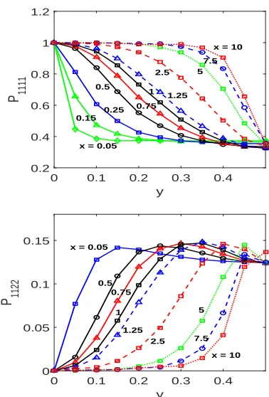
Figs. 6 describes the distribution of two components P1111 (Top figure) and P1122 (Bottom figure) of the fourth-order
y
0 0.1 0.2 0.3 0.4 0.5
Outlet velocity profile [u]
0 0.5 1 1.5
Newtonian case
φµ/η0 = 2
φµ/η0 = 6
φµ/η0 = 10
Figure 5: Flow of fibre suspensions between two parallel plates: the velocity profile at the outlet of the Newtonian fluid flow and the fibre suspension flows with kf = (2,6,10).
tensorhPPPPion the width of the channel as well as along the channel. The distribution shows that fibres have a ten-dency to be associated to the flow direction (x-direction in this example) when approaching the outlet. In other words, the components P1111and P1122of tensor P converge to unity and zero, respectively at the region near the outlet. Fur-thermore, the isotropic state of fibre configurations is mostly maintained on the centreline along the channel.
y
0 0.1 0.2 0.3 0.4
P 1111
0.2 0.4 0.6 0.8 1 1.2
x = 10
0.15 0.25 0.5
0.75 1 1.25
2.5 5 7.5
x = 0.05
y
0 0.1 0.2 0.3 0.4
P 1122
0 0.05 0.1
0.15 x = 0.05
x = 10 0.5
0.75
1
1.25 2.5
5
7.5
Figure 6: Flow of fibre suspensions between two parallel plates: the distribution of the components P1111(Top figure) and P1122(Bottom figure) along the channel with kf =10.
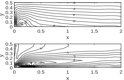
[image:5.595.333.522.375.654.2] [image:5.595.65.254.502.649.2]Txyand Txx−Tyyas well as their values are close match with those byChiba et al.(2001).
x
0 0.5 1 1.5 2
y
0 0.1 0.2 0.3 0.4
0.5 0
2
4
6 8
10 12
x
0 0.5 1 1.5 2
y
0 0.1 0.2 0.3 0.4 0.5
-1
-1
1 3 5 7
[image:6.595.50.267.78.218.2]9 11
Figure 7: Flow of fibre suspensions between two parallel plates: The distribution of shear stress (Top figure) and the first normal stress difference (Bottom Figure) in flow with kf =10.
Finally, the orientation of fibres along the channel is de-scribed by ellipses whose shape and major axes are deter-mined by the eigenvalues and eigenvectors of the second-order orientation tensorhPPi. For example, a circular ellipse implies a fibres’ isotropic direction at a collocation point, while a horizontal straight-line ellipse indicates that all fi-bres at that point completely align with the flow direction. Fig. 8shows the evolution of the fibres’ orientation along the channel. The result shows that the fibres’ orientation is strongly impacted by the shear stress field of the flow along the channel (see Fig. 7, Top)and the boundary conditions for fibre configurations at the inlet and the wall. Indeed, the isotropic orientation is maintained at the inlet and the centre-line, where having the zero-value shear stress. This isotropic state is gradually reduced to the completely alignment state when approaching the wall, where the maximum shear stress exists.
x
0 0.5 1 1.5 2
y
[image:6.595.54.289.495.576.2]0 0.2 0.4
Figure 8: Flow of fibre suspensions between two parallel plates: the evolution of the fibres’ orientation from the in-let x=0 to x=2 in flow with kf=10.
CONCLUSION
This paper reports the use of a 1D-IRBF-BCF method to simulate dilute fibre suspension flows. At a time step, all governing differential equations including the vorticity trans-port equation and the Jeffery’s equation of fibre configura-tion fields are separately solved using the 1D-IRBF method. The evolution of fibre configurations captured by the Jef-fery’s equation is approximated using the BCF idea. The two processes are closed by Lipscomb’s model. The significant contribution of this work is to integrate the 1D-IRBF scheme into the numerical approximation of two phases solvent and fibres. Taking the advantages of the method, the stability and
the accuracy of solutions are significantly improved. Indeed, the obtained results by simulating the fibre suspension flow through a channel including velocity, stress and the distribu-tion of fibre configuradistribu-tion are in very good agreement with those of Chiba et al. (2001) whereas the convergence mea-sure is significantly improved even with a coarser mesh used.
ACKNOWLEDGEMENT: The first author would like to thank USQ for a Postgraduate Research scholarship and Scholarship Sup-plements by FoHES and CESRC. These supports are gratefully ac-knowledged.
REFERENCES
ADVANI, S. et al. (1987). “The use of tensors to describe and predict fiber orientation in short fiber composites”. Journal of
Rhe-ology (1978-present), 31(8), 751–784.
CHIBA, K. et al. (2001). “Numerical solution of fiber suspen-sion flow through a parallel plate channel by coupling flow field with fiber orientation distribution”. Journal of non-newtonian fluid
mechanics, 99(2), 145–157.
CINTRA JR, J.S. and TUCKER III, C.L. (1995). “Orthotropic closure approximations for flow-induced fiber orientation”. Journal
of Rheology (1978-present), 39(6), 1095–1122.
DOU, H.S. et al. (2007). “Simulations of fibre orientation in dilute suspensions with front moving in the filling process of a rect-angular channel using level-set method”. Rheologica acta, 46(4), 427–447.
FAN, X.J. et al. (1999). “Simulation of fibre suspension flows by the brownian configuration field method”. Journal of non-newtonian fluid mechanics, 84(2), 257–274.
FERREIRA, V.G. et al. (2002). “High-order upwinding and the hydraulic jump”. International journal for numerical methods in
fluids, 39(7), 549–583.
HULSEN, M.A. et al. (1997). “Simulation of viscoelastic flows using brownian configuration fields”. Journal of Non-Newtonian
Fluid Mechanics, 70(1), 79–101.
LIPSCOMB, G.G. et al. (1988). “The flow of fiber suspensions in complex geometries”. Journal of Non-Newtonian Fluid Mechanics,
26(3), 297–325.
LU, Z. et al. (2006). “Numerical simulation of fibre suspension flow through an axisymmetric contraction and expansion passages by brownian configuration field method”. Chemical engineering
science, 61(15), 4998–5009.
MAI-DUY, N. and TRAN-CONG, T. (2001). “Numerical solu-tion of differential equasolu-tions using multiquadric radial basis func-tion networks”. Neural Networks, 14, 185–199.
MAI-DUY, N. and TRAN-CONG, T. (2007). “A collocation method based on onedimensional rbf interpolation scheme for solv-ing pdes”. International Journal of Numerical Methods for Heat
and Fluid Flow, 26, 426–447.
NGUYEN, H.Q. et al. (2015). “RBFN stochastic coarse grained simulation method: PartI - Dilute polymer solutions using Bead-Spring Chain models”. CMES: Computer Modeling in Engineering
& Sciences.
PHAN-THIEN, N. and GRAHAM, A.L. (1991). “A new consti-tutive model for fibre suspensions: flow past a sphere”. Rheologica
acta, 30(1), 44–57.
SZERI, A.J. and LEAL, L.G. (1994). “A new computational method for the solution of flow problems of microstructured flu-ids. part 2. inhomogeneous shear flow of a suspension”. Journal of
Fluid Mechanics, 262, 171–204.
TRAN, C.D. et al. (2011). “An integrated RBFN-based macro-micro multi-scale method for computation of visco-elastic fluid flows”. CMES: Computer Modeling in Engineering and Sciences,
82(2), 137–162.
TRAN, C.D. et al. (2012). “A continuum-microscopic method based on IRBFs and control volume scheme for viscoelastic fluid flows”. CMES: Computer Modeling in Engineering and Sciences,