Perturbative Renormalisation of the Second Moment of Generalised Parton Distributions

arXiv:hep-lat/0410009v1 6 Oct 2004

DESY 04-197 Edinburgh 2004/25 Leipzig LU-ITP 2004/023 Liverpool LTH 637

Perturbative Renormalisation of the Second

Moment of Generalised Parton Distributions

M. G¨ockeler

, R. Horsley

, H. Perlt

, P. E. L. Rakow

, A. Sch¨afer

,

G. Schierholz

and A. Schiller

1 _{Institut f¨ur Theoretische Physik, Universit¨at Leipzig,}

D-04109 Leipzig, Germany

2 _{Institut f¨ur Theoretische Physik, Universit¨at Regensburg,}

D-93040 Regensburg, Germany

3 _{School of Physics, University of Edinburgh, Edinburgh EH9 3JZ, UK} 4 _{Theoretical Physics Division, Department of Mathematical Sciences,}

University of Liverpool, Liverpool L69 3BX, UK 5 _{John von Neumann-Institut f¨ur Computing NIC,}

Deutsches Elektronen-Synchrotron DESY, D-15738 Zeuthen, Germany 6 _{Deutsches Elektronen-Synchrotron DESY, D-22603 Hamburg, Germany}

Abstract

1

Introduction

In recent years generalised parton distributions (GPDs) [1] became a focus of both ex-perimental and theoretical studies in hadron physics. For an extensive up-to-date review including a comprehensive list of references see [2]. GPDs provide a universal (with the meaning used in factorisation proofs), unifying parametrisation for a large class of hadronic correlators, including e.g. form factors and the ordinary parton distribution functions. Thus they provide a solid formal basis to connect information from various inclusive, semi-inclusive and exclusive reactions in an efficient, unambiguous manner. Furthermore they give access to physical quantities which cannot be directly determined in experiments, like e.g. the orbital angular momentum of quarks and gluons in a nucleon (for a chosen specific scheme) and the spatial distribution of the energy or spin density of a fast moving hadron in the transverse plane. This enormous potential motivates the ongoing dedicated investigation of exclusive reactions at DESY, CERN, JLab and other accelerator centers [3, 4]. As GPDs are well-defined QCD objects it was possible to derive many fundamental theoretical results, e.g. the form of their NLO-Q2_{-evolution equations} as well as the NLO coefficient functions for Deeply Virtual Compton Scattering.

However, the direct experimental access to GPDs beyond the limiting cases of distri-bution functions and simple form factors is limited. So one can at most hope to compare experimental data with suitable parametrisations or models. But even under the most optimistic assumptions one would certainly need of the order of 20 parameters per flavour for a reliable fit of all GPDs. (Basically, because GPDs contain so much physics they cannot be expected to be trivial functions.) Another practical problem is that exclusive cross sections typically fall so rapidly with Q2 _{that only moderate Q}2 _{values can be} stud-ied. For these, however, higher-twist contributions can be sizeable, which complicates the situation even further.

More precisely we can write [5] for example

hp′|Oµ1···µn|pi = ¯u(p

′_)γ

(µ1u(p)

[n₋1 2 ]

X

i=0

An,2i(t)∆µ2· · ·∆µ2i+1pµ2i+2· · ·pµn)

− 1 2Mu¯(p

′_)i∆α_σ

α(µ1u(p)

[n₋1 2 ]

X

i=0

Bn,2i(t)∆µ2· · ·∆µ2i+1pµ2i+2· · ·pµn) (1)

+ Cn(t)Mod(n+ 1,2)

1

Mu¯(p

′_)u(p)∆

(µ1· · ·∆µn),

where all indices are symmetrised and trace terms are subtracted as indicated by (· · ·). The leading twist-two operators used in (1) are

Oµ1···µn =

i

2

n−1

¯

ψγ(µ1

↔

Dµ2 · · ·

↔

Dµn) ψ (2)

with the symmetric covariant derivative

↔

D=D→ −D .← (3)

Analogous equations exist for

O_µ51···µn =

i

2

n−1

¯

ψγ(µ1

↔

Dµ2 · · ·

↔

Dµn) γ5ψ (4)

and for the tower of operators involving σµν (related to the generalised transversity) [6].

In (1) we have the nucleon 4-momentum transfer ∆ = p′_{−p and its invariant t = ∆}2_,

p= (p′_{+p)/2 denotes the average nucleon momentum and M its mass.}

The generalised form factors An,2i(t), Bn,2i(t) and Cn(t) are related to the moments

of the GPDs by1

Z 1

−1

dx xn−1H(x, ξ, t) = [n₋1

2 ]

X

i=0

An,2i(t)(−2ξ)2i+ Mod(n+ 1,2)Cn(t)(−2ξ)n,

Z 1

−1

dx xn−1E(x, ξ, t) = [n₋1

2 ]

X

i=0

Bn,2i(t)(−2ξ)2i−Mod(n+ 1,2)Cn(t)(−2ξ)n. (5)

1

The variable ξ =−n·∆/2 is defined with the help of a light-like vector nµ _{which obeys}

p·n= 1.

First results for moments of GPDs obtained on the lattice were published recently [7, 8] (see also [9]) and soon results from improved calculations should become available. Not surprisingly, a number of theoretical problems still has to be settled. One urgent task is to obtain the missing renormalisation factors and to completely analyse the operator mixing. The renormalisation of the operators which are related to (generalised) parton distributions has been discussed extensively, both in the continuum and on the lattice. Up to now, however, almost exclusively the case of forward matrix elements has been considered. When non-forward matrix elements are studied, new features arise, which make a reconsideration of the renormalisation problem necessary. In particular, the mixing with “external ordinary derivatives”, i.e. with operators of the form ∂µ∂ν· · · ψ¯· · ·ψ

, needs to be investigated [11]. They do not contribute in forward matrix elements, but have to be taken into account when calculating e.g. the generalised form factors An,2i(t)

for i >0.

On the lattice the mixing patterns are usually more complicated than in the continuum, because covariance under the hypercubic group H(4) imposes less stringent restrictions than O(4) covariance. The necessity to consider also operators with external ordinary derivatives enlarges the set of contributing operators even further. These complications do not yet arise forn= 1 andn = 2. Hence for these moments the renormalisation factors can be taken over from the forward case.

In this paper we investigate the renormalisation problem for n= 3 within the frame-work of one-loop lattice perturbation theory. Some first results have been presented recently [10]. We find that the numerical values of the renormalisation factors are not very different from one. We also find that the pattern of operator mixing is far more involved than e.g. for moments of the ordinary parton distributions. While the numerical results from one-loop lattice perturbation theory have limited precision, the results con-cerning the mixing of operators are valid in general. Note also that our considerations apply equally well to moments of distribution amplitudes.

Let us fix the notations used in our perturbative calculations. We work in Euclidean space and use the Wilson gauge action and Wilson fermions such that the total action is given by

The fermionic part SW,F for dimensionful massless fermion fields ψ(x) has the form

SW,F = 4a3r

X

x

¯

ψ(x)ψ(x)

− a 3

2

X

x,µ

¯

ψ(x)(r−γµ)Ux,µψ(x+aµˆ) + ¯ψ(x+aµˆ)(r+γµ)Ux,µ† ψ(x)

,

where a is the lattice spacing and the sums run over all lattice sites x and directions µ

on the lattice (all other indices are suppressed). The link matricesUx,µ are related to the

gauge field Aµ(x) by

Ux,µ = exp [igaAµ(x)], Aµ(x) =TcAcµ(x),

where g is the bare gauge coupling and the Tc _{are the generators of the SU(3) algebra.}

The Wilson parameter r can be chosen from the interval (0,1]. The gauge action for the gluon field Aµ(x) is

SW,G= 6

g2

X

x,µ<ν

1− 1

6Tr Ux,µν+U †

x,µν

with

Ux,µν =Ux,µUx+aµ,νˆ Ux†+aν,µˆ Ux,ν† .

In the perturbative calculation the investigated operators are sandwiched between off-shell quark states. We shall denote the momentum of the incoming quark by p and that of the outgoing quark by p′_{. Our calculations are performed in Feynman gauge, the final} numbers will be presented for the Wilson parameter r= 1.

2

Operators and mixing

2.1

Renormalisation and mixing in the one-loop approximation

In this section we discuss renormalisation and mixing in general terms, on the lattice as well as in the continuum.

Let ΓD

dimensions. The corresponding Born terms are denoted by ΓBorn

j (p′, p). The operators

potentially contributing to the mixing have to satisfy certain symmetry requirements. They should transform identically according to a given irreducible representation ofO(4) orH(4), respectively, and they should have the same charge conjugation parity.

The (dimensionless) renormalised coupling constantgR is related to the (dimensionful) bare coupling constant g by

g_R2 =µ−2ǫg2 1 +O(g2)

, (6)

where µ is the renormalisation scale. In one-loop perturbation theory we get results of the form

ΓD_j (p′, p, µ, gR, ǫ) = ΓBornj (p′, p)

+g2_R

" _N X

k=1

γ_jkV

1

ǫ −γE + ln(4π)−ln

(p′_+p)2 4µ2

ΓBorn_k (p′, p) +fj(p′, p)

#

+O(g4_R),

(7) whereγE = 0.5772. . . is Euler’s constant. As usual, contributions which vanish forǫ →0

have been omitted. In what follows, we systematically omit all contributions O(g4 R). In the MS scheme the renormalised vertex functions are then given by

ΓR_j(p′, p, µ, gR) = ΓBorn_j (p′, p)

+g2_R

" _N X

k=1

γ_jkV ·(−1)·ln(p ′_+p)2

4µ2 Γ Born

k (p′, p) +fj(p′, p)

#

. (8)

In the absence of mixing with lower-dimensional operators the vertex functions regu-larised on a lattice can be written as

ΓL_j(p′, p, a, gR) = ΓBornj (p′, p)

+g2 R

" _N X

k=1

γV

jk·(−1)·ln

a2_(p′_+p)2

4 Γ

Born

k (p′, p) +fjL(p′, p)

#

(9)

up to terms vanishing asa →0. There should be anN×N matrixζ such that the relation between the bare lattice vertex functions and the MS renormalised vertex functions can be written as

ΓR_j(p′, p, µ, gR) =

N

X

k=1

δjk+gR2ζjk

ΓL_k(p′, p, a, gR). (10)

So we should have

ΓR_j (p′, p, µ, gR) = ΓBorn_j (p′, p)

+g_R2

" _N X

k=1

ζjk−γjkV ln

a2_(p′_+p)2 4

ΓBorn_k (p′, p) +f_jL(p′, p)

#

Comparing with (8) we arrive at

N

X

k=1

ζjk−γVjkln a2µ2

ΓBorn_k (p′, p) +f_jL(p′, p)−fj(p′, p) = 0. (12)

As this equation must hold for arbitrary momenta p′_{, p, there should be constants c}V jk

such that

f_jL(p′, p)−fj(p′, p) = N

X

k=1

cV_jkΓBorn_k (p′, p). (13)

This fixes the matrix ζjk:

ζjk =γVjkln a2µ2

−cV_jk. (14) If the coefficients cV

jk are uniquely determined, exactly all N operators mix to one-loop

accuracy. It might happen that certain operators contribute to mixing only in higher orders. In that case N is decreased. If Eq. (13) cannot be satisfied, this shows that at least one mixing operator has been overlooked.

Mixing with lower-dimensional operators leads to the appearance of additional terms on the r.h.s. of Eq. (9). For example, consider the case of a single operator which mixes with Oj and whose dimension is one unit smaller. (Such a case will appear in our

appli-cations.) Then we get instead of (9)

ΓL_j(p′, p, a, gR) = ΓBorn_j (p′, p)

+g_R2

" _N X

k=1

γ_jkV ·(−1)·lna

2_(p′_+p)2

4 Γ

Born

k (p′, p) +

1

acjΓ

Born_(p′_{, p) +f}L j (p′, p)

#

, (15)

where ΓBorn_(p′_{, p) is the Born term of the additional lower-dimensional operator. The} 1/a contribution has to be subtracted from ΓL

j(p′, p, a, gR) before the connection with

ΓR

j(p′, p, µ, gR) can be established, i.e. in (10) ΓLk(p′, p, a, gR) has to be replaced by

ΓL

k(p′, p, a, gR)−

g2 R

a ckΓ

Born_(p′_{, p). (16)}

Then Eq. (13) is obtained as before.

In order to compute the matrixZjkof renormalisation and mixing coefficients we note

that the connection between the bare lattice vertex functions and the MS renormalised vertex functions can be written as

ΓR_j(p′, p, µ, gR) = Z_ψ−1

N

X

k=1

with the quark wave function renormalisation constant2 _Z

ψ. (In the presence of

mix-ing with a lower-dimensional operator, ΓL

k(p′, p, a, gR) has again to be replaced by the subtracted expression (16)). Comparison with (10) yields

Z_ψ−1Zjk=δjk+gR2ζjk. (18)

The quark wave function renormalisation constant is calculated from the quark prop-agator. Write the lattice regularised inverse quark propagator in Feynman gauge (after subtracting a linearly diverging contribution∼1/a) as

S_L−1(p) = i6p

1 + g 2

RCF

16π2 −ln a 2_p2

−σL

(19)

where σL = 11.8524 (see e.g. [16]) for Wilson fermions. In dimensional regularisation the

inverse quark propagator is given by

S_D−1(p) = i6p

1 + g 2

RCF

16π2

1

ǫ −γE + ln(4π)−ln p2

µ2 + 1

(20)

and we get for the MS renormalised propagator

S_R−1(p) =i p/

1 + g 2

RCF

16π2

−ln p 2

µ2 + 1

. (21)

Defining Zψ such that

S_R−1(p) =Z_ψ−1S_L−1(p) (22)

we have

Zψ = 1−

g2

RCF

16π2 ln a 2_µ2

+ 1 +σL

. (23)

With the help of this result we get from (14) and (18) for the matrix of the renormalisation and mixing coefficients

Zjk =δjk+g2R

γV_jk−δjk

CF

16π2

ln a2µ2

−cV_jk−δjk

CF

16π2(1 +σL)

. (24)

The basic computational task is thus to find the functions fj(p′, p) and fjL(p′, p) in

Eqs. (7) and (9) (or rather their difference). Then we can compute the coefficients cV jk

from Eq. (13) and use Eq. (24) to get the desired renormalisation and mixing coefficients. If we are only interested in the renormalisation of one particular operator, corresponding toj = 1 say, it is sufficient to restrict the calculations to the case j = 1.

2

2.2

Contributing operators for special representations

Let us introduce the self-explaining notations for operators with covariant and external ordinary derivatives

ODD_µνω = −1 4ψγ¯ µ

↔

Dν

↔

Dω ψ ,

O∂D_µνω = −1 4∂ν

¯

ψγµ

↔

Dω ψ

, (25)

O∂∂_µνω = −1

4∂ν∂ω ψγ¯ µψ

and

O_µνω5,DD = −1 4ψγ¯ µγ5

↔

Dν

↔

Dω ψ ,

O5_µνω,∂D = −1 4∂ν

¯

ψγµγ5 ↔

Dω ψ

, (26)

O_µνω5,∂∂ = −1

4∂ν∂ω ψγ¯ µγ5ψ

,

as well as the lower-dimensional operators

OD_µνω =−i

2ψ¯[γµ, γν] ↔

Dω ψ , Oµνω∂ =−

i

2∂ω ψ¯[γµ, γν]ψ

. (27)

For completeness we include here also operators contributing to non-forwardtransversity

matrix elements with two derivatives which were not considered in Eqs. (2) and (4):

OT,DD_µνωσ =−1

4ψ¯[γµ, γν] ↔

Dω

↔

Dσ ψ , OT,∂∂µνωσ =−

1

4∂ω∂σ ψ¯[γµ, γν]ψ

. (28)

As short-hand notations we use in the following (cf. [12])

O{ν1ν2ν3} =

1

6(Oν1ν2ν3 +Oν1ν3ν2 +Oν2ν1ν3 +Oν2ν3ν1 +Oν3ν1ν2 +Oν3ν2ν1) , (29)

Okν1ν2ν3k = Oν1ν2ν3 − Oν1ν3ν2 +Oν3ν1ν2 − Oν3ν2ν1 −2Oν2ν3ν1+ 2Oν2ν1ν3, (30)

Ohhν1ν2ν3ii = Oν1ν2ν3 +Oν1ν3ν2 − Oν3ν1ν2 − Oν3ν2ν1. (31)

First we consider the operator

O_{124}DD =−1 4ψγ¯ {1

↔

D2 ↔

Its charge conjugation parity is C = −1 and it is a member of an irreducible multiplet of operators transforming according to the representation τ₂(4) of H(4) [12]. Here τ_k(l)

denotes an irreducible representation of H(4) with dimension l, and k = 1,2, . . . labels inequivalent representations of the same dimension. This operator can only mix with

O_{124}∂∂ =−1

4∂{2∂4 ψγ¯ 1}ψ

. (33)

Next we examine the operator

O1 =ODD{114}− 1 2 O

DD

{224}+O{334}DD

. (34)

It has already been used in lattice computations of forward hadronic matrix elements, because in this case it suffers only from rather mild mixing problems. It belongs to the representation τ1(8) with C =−1.

Taking into account also external ordinary derivatives, one finds the following opera-tors which transform identically and could therefore mix with (34)3_:

O2 =O_{114}∂∂ − 1 2 O

∂∂

{224}+O{334}∂∂

,

O3 =O_hh114iiDD − 1 2 O

DD

hh224ii+Ohh334iiDD

,

O4 =Ohh114ii∂∂ − 1 2 O

∂∂

hh224ii+Ohh334ii∂∂

, (35)

O5 =O_||213||5,∂D ,

O6 =O_hh213ii5,∂D ,

O7 =O||213||5,DD

and the lower-dimensional operator

O8 =O∂₄₁₁−1 2 O

∂

422+O433∂

. (36)

As an “axial” analogue of (32) we consider the operator O_{124}5,DD

O_{124}5,DD =−1 4ψγ¯ {1

↔

D2 ↔

D4}γ5ψ , (37)

3

The charge conjugation paritiesC ofO7 andO5coincide sinceO7 is antisymmetric in the indices of

which can mix with

O5_{124},∂∂ =−1

4∂{2∂4 ψγ¯ 1}γ5ψ

. (38)

(37) and (38) belong to τ₃(4) with C = +1.

Similarly, we have as a counterpart of (34) the operator

O5₁ =O_{114}5,DD− 1 2

O_{224}5,DD+O5_{334},DD . (39)

Its charge conjugation parity isC = +1 and it is a member of an irreducible multiplet of operators transforming according the representation τ2(8) of H(4) [12].

The following operators with identical transformation behaviour could potentially mix with (39):

O5₂ =O_{114}5,∂∂ − 1 2

O5_{224},∂∂ +O_{334}5,∂∂ ,

O5₃ =O_hh114ii5,DD − 1 2

O_hh224ii5,DD +O5_hh334ii,DD ,

O5₄ =O_hh114ii5,∂∂ − 1 2

O_hh224ii5,∂∂ +O5_hh334ii,∂∂ , (40)

O5₅ =O_||213||∂D ,

O5₆ =O_hh213ii∂D ,

O5₇ =O_||213||DD

and the lower-dimensional operator

O₈5 =OD₁₂₃−2OD₂₃₁− OD₁₃₂. (41)

For the operators (28) we consider the representations τ₂(3), τ₃(3) and τ₂(6) with C = −1 [13]. In the case of τ₂(3) we choose the representative operator

OT₁ =OT,DD_4{123}, (42)

which may mix with

OT2 =OT,∂∂4{123}. (43)

For τ₃(3) we take

mixing with

OT

4 =−O

T,∂∂

1{133} +O

T,∂∂

1{144}− O

T,∂∂

2{233}+O

T,∂∂

2{244}−2O

T,∂∂

3{344}. (45)

The operator

O₅T =OT,DD_13{32}+O_23{31}T,DD − O_14{42}T,DD − O_24{41}T,DD (46)

belonging to the representation τ₂(6) also mixes with only one additional operator:

O₆T =OT,∂∂_13{32}+O_23{31}T,∂∂ − O_14{42}T,∂∂ − O_24{41}T,∂∂ . (47)

Other representations show a more complicated mixing behaviour and will be not consid-ered here.

3

One-loop calculation of non-forward matrix

ele-ments

3.1

Calculational technique

We calculate the matrix elements of the operators in one-loop lattice perturbation theory in the infinite volume limit following Kawai et al. [14]. The computation is performed symbolically adopting and significantly extending aMathematica program package devel-oped originally for the case of moments of structure functions using Wilson [15], clover [16] and overlap fermions [17].

Using that approach we have full analytic control over pole cancellation. The Lorentz index structure of the matrix elements is left completely free, so that we are able to construct all representations of the hypercubic group for the second moments in the non-forward case. The analytic derivation is disconnected from the numerical calculation of

finite lattice integrals. These integrals are calculated to a high accuracy and are given as look-up tables.

To be more precise, we recapitulate in short the strategy [14, 15] for calculating the diagrams adapted to our case of two distinct external momentap6=p′_{. Basically we have} to evaluate a typical lattice integral of the form

Iµ1···µn(a, p ′_{, p) =}

Z π/a

−π/a

d4_k

(2π)4 Kµ1···µn(a, p

where the integration is performed over the first Brillouin zone. The numerator of the kernel Kµ1···µn(a, p

′_{, p, k) is a polynomial in sines and cosines of the lattice momenta k,} the denominator contains the denominators of lattice quark and gluon propagators. Such an integral I is calculated by splitting it into two parts

I = ˜I+ (I −I)˜ . (49)

Here ˜I denotes the Taylor expansion of the original integral I in the external momenta ˜

I(a, p′, p) = I(a,0,0)

+ X

α

p′_α∂I(a, p

′_{, p)}

∂p′

α

p′_=p=0+pα

∂I(a, p′_{, p)}

∂pα

p′_=p=0

+. . . (50)

where the order of the expansion is given by the degree of ultraviolet (UV) divergence ofI. As a consequence, the differenceI −I˜is UV finite and can be calculated in the (Euclidean) continuum, taking the limit a → 0. The original UV poles appear now as infrared (IR) poles in the Taylor expansion and are regularised using dimensional regularisation with

d >4. Since in that case ˜I|a→0 vanishes, we have (I −I)|˜ a→0 =I|a→0 ≡ Icont(p′, p) and the second contribution to the final lattice result is just a one-loop continuum calculation in dimensional regularisation.

The first (Taylor expanded) part is calculated in d = 4−2ǫ dimensions at finite a, the poles in ǫ analytically cancel those of the second part Icont_{. Note that the first part} depends on the external momenta only via the Taylor expansion, therefore the lattice integrals (the expansion coefficients) are just numbers (independent ofp and p′_).

In the Euclidean continuum part Icont_(p′_{, p) the finite contribution depends on the} (different) external momenta in a complicated manner. As in Minkowski space, the finite part of three-point functions with three different propagators is difficult to represent in a simple compact analytic form (see, e.g., [18]). In parametrising that contribution we have chosen the following form

I_µcont1···µn(p

′_{, p) =} 1

ǫAµ1···µn(p

′_{, p) +} X

i,j,k,m

Bµ1···µn(p

′_{, p, i, j, k, m)F(i, j, k, m, p}′_{, p). (51)}

In (51) the functionsAµ1···µn(p

′_{, p) (known analytically) andB}

µ1···µn(p

′_{, p, i, j, k, m) contain} the general index structure assigned to the external momenta p and p′_{. The symbols F} stand for the remaining integrals (finite forp6=p′_{) over the Feynman parameters}4_:

F(i, j, k, m, p′, p) =

Z 1

0

dx

Z 1−x

0

dy xiyj Q2(x, y, p′, p)k

lnm Q

2_{(x, y, p}′_{, p)}

µ2 (52)

4

with

Q2_{(x, y, p}′_{, p) =p}2_{x(1−x) +p}′2_{y(1−y)−2p·p}′_{x y .}

Only few combinations of the integers i, j, k, m are actually needed in the “continuum part” of the one-loop calculation. But compact expressions for the F(i, j, k, m, p′_{, p) do} not seem to exist.

As we have shown in Section 2.1, in order to calculate the finite renormalisation matrix converting the lattice result to the MS scheme we have to find the difference between the lattice and the continuum one-loop contribution fL

j (p′, p)−fj(p′, p), and similarly for the

wave function renormalisation. Therefore, we do not need the explicit form of the finite continuum one-loop contribution (which is essentially given by the F’s), since it cancels exactly the part coming from the second term of (49). As a consequence, we do not present F-integrals here. However, choosing other schemes, the finite contributions to Iµ1···µn(p

′_{, p)}cont _{might be needed.}

3.2

One-loop renormalisation matrices for the chosen

represen-tations

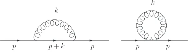
To calculate the one-loop contributions for the above operators between quark states we have to take into account self energy and amputated Green function diagrams. The quark self energy diagrams (contributing to the quark wave function renormalisation) are shown in Fig. 1. Denoting the operator insertions by a black dot, the vertex and tadpole

p p+k p

k

p p

k

Figure 1: One-loop diagrams contributing to the quark self-energy.

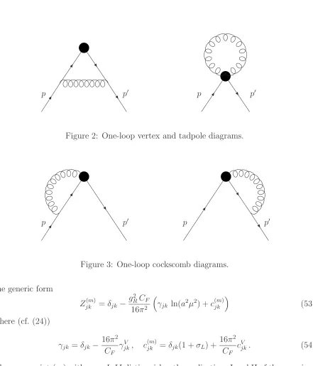
diagrams (Fig. 2) as well as the “cockscomb” diagrams (Fig. 3) contribute in one-loop order to the amputated Green functions.

p p′ _{p p}′

Figure 2: One-loop vertex and tadpole diagrams.

p p′ _{p p}′

Figure 3: One-loop cockscomb diagrams.

the generic form

Z_jk(m) =δjk−

g2

RCF

16π2

γjk ln(a2µ2) +c(jkm)

(53)

where (cf. (24))

γjk =δjk−

16π2 CF

γ_jkV , c(_jkm) =δjk(1 +σL) +

16π2 CF

cV_jk. (54)

3.2.1 ODD

{124}(τ (4)

2 , C =−1)

For this representation we find mixing between ODD

{124} (32) and O∂∂{124} (33). The corre-sponding 2×2-mixing matrices are

γjk=

₂₅

6 − 5 6

0 0

, (55)

c(_jkI,II) =

−11.5632 0.0241 0 20.6178

. (56)

The anomalous dimension matrix was calculated earlier [11]. The elementc11=−11.5632 in the matrix (56) is known from our previous calculation in the forward case [15] andc22 comes from the renormalisation of the local vector current [16]. The matrix c(_jkI,II) shows a very small mixing between the operatorsODD

{124} andO∂∂{124}. Thus it may be justified to neglect the mixing in practical applications.

3.2.2 O1(τ₁(8), C =−1)

We consider the mixing of operators having the same dimension first. The relevant oper-ators have been defined in Section 2.2. To one-loop accuracy the operatorO7 in Eq. (35) does not contribute and we have to consider the following mixing set:

{O1,O2,O3,O4,O5,O6}.

The anomalous dimension matrix is

γjk=



      

25 6 −

5

6 0 0 0 0

0 0 0 0 0 0

0 0 7₆ −5₆ 1 −3₂

0 0 0 0 0 0

0 0 0 0 2 −2

0 0 0 0 −2₃ 2₃



      

(57)

and the finite part of the mixing matrix is given by

c(_jkI) =



      

−12.1274 −2.7367 0.3685 0.9934 0.0156 0.1498

0 20.6178 0 0 0 0

3.3060 18.1841 −14.8516 −4.3023 −0.9285 0.7380

0 0 0 20.6178 0 0

0 3.2644 0 0 0.3501 0.0149 0 3.2644 0 0 0.0050 0.3600



      

or

c(_jkII) =



      

−12.1274 1.4913 0.3685 −0.4160 0.0156 0.1498

0 20.6178 0 0 0 0

3.3060 −8.01456 −14.8516 4.3023 −0.9285 0.7380

0 0 0 20.6178 0 0

0 3.2644 0 0 0.3501 0.0149

0 3.2644 0 0 0.0050 0.3600



      

. (59)

The matrices c(_jkI,II) show a sizeable mixing of the operator O1 with other operators, especiallyO2 containing two external ordinary derivatives. This mixing becomes irrelevant in the forward case, where the matrix element of O2 vanishes. On the other hand, the mixing between the operatorsO1 and O3 is already known from our previous calculations in the forward case [15].

There is also a possible mixing betweenO1 and the lower-dimensional operatorO8(36). Indeed, we find in the one-loop approximation that the vertex function of O1 contains a term ∝1/a:

O1

1

a−part = g

2

RCF

16π2 (−0.5177) 1

aO

Born

8 . (60)

This mixing leads to a contribution which diverges like the inverse lattice spacing in the continuum limit. The operator O8 has to be subtracted non-perturbatively from the operator O1 which might be a difficult task in simulations.

3.2.3 O5_{124},DD(τ₃(4), C = +1)

For this representation we find mixing between O5_{124},DD andO_{124}5,∂∂ . The anomalous dimen-sion matrix is given by (55), the finite contributions are collected in the matrix

c(_jkI,II) =

−12.1171 0.1667 0 15.7963

. (61)

As in the case of the operator ODD

3.2.4 O5 1(τ

(8)

2 , C = +1)

First we discuss the mixing of operators of the same dimension. The set of contributing operators is found to be

{O₁5,O₂5,O5₃,O₄5,O₅5,O5₆}.

As in the case of the operatorO1, one operator – hereO57 – does not contribute to mixing in one-loop order. The finite contributions for the two lattice derivatives are

c(_jkI) =

       

−12.8609 −2.0653 0.3490 0.8538 0.0511 0.0594

0 15.7963 0 0 0 0

3.4220 15.8207 −15.3592 −5.1639 0.1701 −0.9431

0 0 0 15.7963 0 0

0 −8.9124 0 0 0.9597 −0.9597 0 −8.9124 0 0 −0.3199 0.3199

        (62) and

c(_jkII)=

       

−12.8609 1.4894 0.3490 −0.3311 0.0511 0.0594

0 15.7963 0 0 0 0

3.4220 −7.3002 −15.3592 2.5431 0.1701 −0.9431

0 0 0 15.7963 0 0

0 −8.9124 0 0 0.9597 −0.9597 0 −8.9124 0 0 −0.3199 0.3199

        . (63)

The anomalous dimension matrix is the same as for the operators without γ5, see (57). Again, some of the mixing coefficients may be non-negligible. The mixing between O5 1 and O5

3 is visible even in the forward case.

We also find mixing with a lower-dimensional operator, in this case it is the operator O5

8 (41). The corresponding contribution in the vertex function ofO15 reads

O51

1 a−part = g 2

RCF

16π2 (−0.2523) 1

aO

5,Born

8 . (64)

3.2.5 OT

1 (τ (3)

2 , C =−1)

For the mixing between the operators OT

1 (42) and OT2 (43) the matrix of anomalous dimensions is given by

γjk=

and the finite contributions are

c(_jkI,II) =

−11.5483 0.2189 0 17.0181

. (66)

3.2.6 OT

3 (τ (3)

3 , C =−1)

The mixing between the operators OT

3 (44) and O4T (45) leads to the same anomalous dimension matrix (65) as the previous case. For the finite pieces we obtain

c(_jkI,II) =

−11.8688 0.2753 0 17.0181

. (67)

3.2.7 OT

5 (τ (6)

2 , C =−1)

For the operatorsOT

5 (46) and O6T (47) we find the finite mixing contributions

c(_jkI,II)=

−11.7477 0.2380 0 17.0181

(68)

with the identical anomalous dimension matrix (65).

4

Summary

For the representations (τ₂(4), C =−1) and (τ₃(4), C = +1) there are only two multiplets of operators of dimension ≤ 5. Actually, they are all of dimension 5, and the mixing pattern is the same as in the continuum. The mixing coefficients turn out to be quite small.

In the case of the representations (τ₁(8), C = −1) and (τ₂(8), C = +1) we have eight multiplets of operators of dimension ≤ 5. In the one-loop approximation one of them cannot yet contribute, but the remaining seven multiplets do actually show up. Six of them are of dimension 5, but there is also one multiplet of operators of dimension 4. For these representations some of the mixing coefficients are larger than in the above cases. In particular the mixing with the lower-dimensional operators, which will probably receive sizeable non-perturbative corrections, might lead to difficulties in the numerical simulations: 1/a effects are hard to get under control.

In the operators just mentioned the Dirac matrix is either γµ orγµγ5. In connection

with (generalised) transversity distributions operators with [γµ, γν] are of interest. Here we

restricted ourselves to cases where only mixing with the external derivative counterparts is possible and found rather small mixing coefficients.

The results presented in this paper were obtained for Wilson fermions. However, nu-merical simulations will be performed with clover or overlap fermions. Therefore, the numbers given in the preceding section can only serve as first hints at the problems which will occur in these calculations, especially the mixing problem. The sets of mixing oper-ators, on the other hand, follow from symmetry arguments and are therefore universally valid, although additional symmetries may lead to further restrictions, e.g. in the case of overlap fermions. It should also be noted that the overall normalisations of the opera-tors are somewhat arbitrary. So some care has to be exercised when using our results in concrete applications.

Acknowledgements

Appendix: Feynman rules

We need Feynman rules for the lattice operators (25), (26) and (28). Denoting the mo-mentum of the outgoing quark by p′_{, that of the incoming quark by p and the incoming} gluon momenta byki, we use the following Fourier decomposition for the quark and gauge

fields,

ψ(x) =

Z

d4_p

(2π)4ψ(p) e ip·x_,

¯

ψ(x) =

Z

d4_p′ (2π)4ψ¯(p

′_{) e}−ip′_·x

, (69)

Aµ(x) =

Z

d4_k

i

(2π)4Aµ(ki) e

iki·(x+aµ/ˆ 2)_,

where the momenta are restricted to the first Brillouin zone.

We use the standard realisation of the covariant derivatives acting to the right and to the left

→

Dµψ(x) =

1 2a

h

Ux,µψ(x+aµˆ)−Ux†−aµ,µˆ ψ(x−aµˆ)

i

,

¯

ψ(x)D←µ =

1 2a

h

¯

ψ(x+aµˆ)U_x,µ† −ψ¯(x−aµˆ)Ux−aµ,µˆ

i

. (70)

The external ordinary derivative is taken as

∂µ ψ¯· · ·ψ

(x) = 1

a

_¯

ψ· · ·ψ

(x+aµˆ)− ψ¯· · ·ψ

(x)

. (71)

There are two convenient ways to define the corresponding operators in momentum space with non-zero momentum transferq. One possibility is to “act” withqat the lattice point x. For the case of one covariant derivative this leads to (setting the Dirac matrix in the operator equal to the unit matrix for simplicity)

¯

ψ D↔µψ

(I)

(q) = X

x

¯

ψ D↔µ ψ

(x) eiq·x

= 1 2a

X

x

¯

ψ(x)Ux,µψ(x+aµˆ)−ψ¯(x+aµˆ)Ux,µ† ψ(x) eiq·x+ eiq·(x+aµˆ)

. (72)

case of one covariant derivative D~) as follows

¯

ψ D→µψ

(q) = 1 2a

X

x

h

¯

ψ(x)Ux,µψ(x+aµˆ) eiq·(x+aµ/ˆ 2)

−ψ¯(x)U_x†_−aµ,νˆ ψ(x−aµˆ) eiq·(x−aµ/ˆ 2)i,

which leads to

¯

ψ D↔µ ψ

(II)

(q)

= 1

a

X

x

¯

ψ(x)Ux,µψ(x+aµˆ)−ψ¯(x+aµˆ)Ux,µ† ψ(x)

eiq·(x+aµ/ˆ 2). (73)

This realisation might be more suitable for numerical simulations. Note that

¯

ψ D↔µψ

(I)

(q) = cosaqµ 2

¯

ψ D↔µ ψ

(II)

(q). (74)

For the external ordinary derivative we use

∂µ ψ¯· · ·ψ

(q) = 1

a

X

x

_¯

ψ· · ·ψ

(x+aµˆ)− ψ¯· · ·ψ

(x)

eiq·(x+aµ/ˆ 2)

= −2i

a sin aqµ

2 ψ¯· · ·ψ

(q). (75)

The corresponding Feynman rules up to O(g2_{) derived from expressions based on (72)} and (73) are marked by the superscripts (I) and (II), respectively.

O(g0₎

O(µνωII),DD = ψ¯(p′)γµψ(p)

1

a2 sin

a(p+p′₎

ν

2 sin

a(p+p′₎

ω

2 ,

O_µνω(I),DD = cosa(p−p ′₎

ν

2 cos

a(p−p′₎

ω

2 O

(II),DD

µνω ,

O_µνω(II),∂D = ψ¯(p′)γµψ(p)

1

a2 sin

a(p−p′₎

ν

2 sin

a(p+p′₎

ω

2 , (76)

O(_µνωI),∂D = cosa(p−p ′₎

ω

2 O

(II),∂D

µνω ,

O_µνω∂∂ = ψ¯(p′)γµψ(p)

1

a2 sin

a(p−p′₎

ν

2 sin

a(p−p′₎

ω

O(g)

O(_µνωII),DD = gX

σ

¯

ψ(p′)γµAσ(k1)ψ(p) cos

a(p+p′₎

σ

2

×1

a

δνσsin

a(p+p′ _−k1)

ω

2 +δωσsin

a(p+p′ _+k1)

ν

2

,

O_µνω(I),DD = cosa(p−p ′ _+k1)

ν

2 cos

a(p−p′_+k1)

ω

2 O

(II),DD

µνω , (77)

O_µνω(II),∂D = gψ¯(p′)γµAω(k1)ψ(p)

1

asin

a(p−p′_+k1)

ν

2 cos

a(p+p′₎

ω

2 .

O(_µνωI),∂D = cosa(p−p ′ _+k

1)ω

2 O

(II),∂D

µνω .

O(g2_{) for the tadpole case k}

2 =−k1

Here we restrict ourselves to the tadpole casek2 =−k1(cf. Fig. 2) as this is all we need in this paper. For general gluon momenta the Feynman rules are much more complicated.

O(_µνωII),DD = g 2

2

X

σ,τ

¯

ψ(p′)γµAτ(−k1)Aσ(k1)ψ(p)

×

(

2δτ νδσωcos

a(p+p′_+k1)

ν

2 cos

a(p+p′_+k1)

ω

2

−(δτ νδσν +δτ ωδσω) sin

a(p+p′₎

ν

2 sin

a(p+p′₎

ω

2

)

,

O_µνω(I),DD = cosa(p−p ′₎

ν

2 cos

a(p−p′₎

ω

2 O

(II),DD

µνω , (78)

O(II),∂D

µνω = −

g2 2ψ¯(p

′_)γ

µAω(k1)Aω(−k1)ψ(p) sin

a(p−p′₎

ν

2 sin

a(p+p′₎

ω

2 ,

O_µνω(I),∂D = cosa(p−p ′₎

ω

2 O

(II),∂D

µνω .

References

[1] D. M¨uller, D. Robaschik, B. Geyer, F. M. Dittes and J. Horejsi, Fortsch. Phys. 42

(1994) 101;

X. D. Ji, Phys. Rev. Lett. 78 (1997) 610, Phys. Rev. D 55 (1997) 7114;

A. V. Radyushkin, Phys. Lett. B 380 (1996) 417, Phys. Lett. B 385 (1996) 333; J. C. Collins, L. Frankfurt and M. Strikman, Phys. Rev. D 56 (1997) 2982.

[2] M. Diehl, Phys. Rept. 388 (2003) 41.

[3] A. Airapetianet al.[HERMES Collaboration], Eur. Phys. J. C17 (2000) 389; Phys. Lett. B 535 (2002) 85;

S. Chekanov et al. [ZEUS Collaboration], Eur. Phys. J. C24 (2002) 345.

[4] A. Airapetian et al. [HERMES Collaboration], Phys. Rev. Lett. 87 (2001) 182001; S. Stepanyan et al. [CLAS Collaboration], Phys. Rev. Lett. 87 (2001) 182002; C. Adloff et al. [H1 Collaboration], Phys. Lett. B 517 (2001) 47;

S. Chekanov et al. [ZEUS Collaboration], Phys. Lett. B 573 (2003) 46.

[5] X. Ji, J. Phys. G 24 (1998) 1181.

[6] P. H¨agler, arXiv:hep-ph/0404138.

[7] M. G¨ockeler, R. Horsley, D. Pleiter, P. E. L. Rakow, A. Sch¨afer, G. Schierholz and W. Schroers [QCDSF Collaboration], Phys. Rev. Lett. 92 (2004) 042002.

[8] P. H¨agler, J. Negele, D. B. Renner, W. Schroers, T. Lippert and K. Schilling [LHPC collaboration], Phys. Rev. D 68 (2003) 034505.

[9] M. G¨ockeler, P. Hagler, R. Horsley, D. Pleiter, P. E. L. Rakow, A. Sch¨afer, G. Schier-holz, J. M. Zanotti, arXiv:hep-lat/0409162.

[10] M. G¨ockeler, R. Horsley, P. E. L. Rakow, H. Perlt, A. Sch¨afer, G. Schierholz and A. Schiller, arXiv:hep-lat/0409025.

[11] G.P. Lepage and S.J. Brodsky, Phys. Rev. D22 (1980) 2157;

A.V. Efremov and A.V. Radyushkin, Theor. Math. Phys. 42 (1980) 97; M.A. Shifman and M.I. Vysotsky, Nucl. Phys. B 186 (1981) 475.

[12] M. G¨ockeler, R. Horsley, E. M. Ilgenfritz, H. Perlt, P. Rakow, G. Schierholz and A. Schiller, Phys. Rev. D 54 (1996) 5705.

[14] H. Kawai, R. Nakayama and K. Seo, Nucl. Phys. B 189 (1981) 40.

[15] M. G¨ockeler, R. Horsley, E. M. Ilgenfritz, H. Perlt, P. E. L. Rakow, G. Schierholz and A. Schiller, Nucl. Phys. B 472 (1996) 309.

[16] S. Capitani, M. G¨ockeler, R. Horsley, H. Perlt, P. E. L. Rakow, G. Schierholz and A. Schiller, Nucl. Phys. B 593 (2001) 183.

[17] R. Horsley, H. Perlt, P. E. L. Rakow, G. Schierholz and A. Schiller, Nucl. Phys. B

693 (2004) 3.

[18] A. I. Davydychev and J. B. Tausk, Phys. Rev. D 53 (1996) 7381;