Towards the Sustainable City: The Impact of Land Use - Transport Interactions. The development of revised location coefficients.

White Rose Research Online URL for this paper: http://eprints.whiterose.ac.uk/2095/

Monograph:

Shepherd, S. (1998) Towards the Sustainable City: The Impact of Land Use - Transport Interactions. The development of revised location coefficients. Working Paper. Institute of Transport Studies, University of Leeds , Leeds, UK.

Working Paper 515

[email protected] https://eprints.whiterose.ac.uk/ Reuse

See Attached

Takedown

If you consider content in White Rose Research Online to be in breach of UK law, please notify us by

White Rose Research Online

Institute of Transport Studies

University of Leeds

This is an ITS Working Paper produced and published by the University of Leeds. ITS Working Papers are intended to provide information and encourage discussion on a topic in advance of formal publication. They represent only the views of the authors, and do not necessarily reflect the views or approval of the sponsors.

White Rose Repository URL for this paper: http://eprints.whiterose.ac.uk/2095

Published paper

1. Development of DELTA location coefficients for Response 5...1

2. Basis of the previous Task 2 Response 1 coefficients...1

2.1 Utility of Consumption and Accessibility coefficients (response 1 task 2) ...2

2.2 Coefficient of Area Quality (response 1 task 2)...2

2.3 Composition of the Environment variable (response 1 task 2)...2

3. Calculation of response 5 coefficients from the stated preference survey. ...3

4. A comparison of response 1 and response 5 coefficients ...7

4.1 Utility of consumption...12

4.2 Accessibility ...12

4.3 Area Quality...12

4.4 Noise ...12

4.5 Pollution ...13

Appendix A : Detail of steps used to produce response 5 coefficients ...17

Step 2 : Produce relationship to income in 1996 for 3 chosen variables from step 1. ...17

Step 5 : Calculation of relationship between accessibility and in-vehicle-time...17

Step 6 : Change Noise units from percentage change to change in dBA...20

Step 7 : Change air quality units to account for START outputs CO, NOX and VOC. ...22

Step 8 : Calculate new utility of consumption coefficient using program UCML11. ...23

Step 11 : Recalculate the area quality coefficient. ...24

1.

Development of DELTA location coefficients for Response 5

This paper gives an outline of the steps undertaken to convert from the willingness to pay for travel time savings, air quality and noise derived in tasks 3 and 4 to the location coefficients for use with the DELTA/START model.

2.

Basis of the previous Task 2 Response 1 coefficients

Before describing the process for developing the new estimates it is useful to review the coefficients and the development of those used in task 2 i.e. response 1.

The land use model DELTA contains a location sub-model which locates and relocates households by maximising their utility of location. The model responds to changes in utility of location and to the amount of space available. The change in utility of location is defined as follows :-

∆V_tih hU U U A A Q Q R R

ti h

t l i

h hA

ti h

t l i

h hQ

ti h

t l i

h hR

ti h

t l i h

=θ ( − _{( −)} )+θ ( − ₍₋₎ )+θ ( − ₍₋₎ )+θ ( − ₍₋₎ ) (2)

where

V_tih = utility of location for households of type h locating in zone i at time t

U_tih = utility of consumption for households of type h locating in zone i at time t

A_tih = accessibility of zone i for households of type h at time t

Q_tih = quality of housing areas for households of type h in zone i at time t

R_tih = transport-related environmental quality as perceived by households of type h in zone i at time t

t-l = time period t-l for lagged variables, l may vary by household type and by variable as required

θhU ₌

coefficient of response to change in utility of consumption for households of type h

θhA =

coefficient of response to change in accessibility for households of type h θhQ =

coefficient of response to change in area quality for households of type h θhR =

coefficient of response to change in transport-related environmental quality for households of type h

2.1 Utility of Consumption and Accessibility coefficients (response 1 task 2)

The four coefficients described above have been estimated from two different sources of data. The coefficients on utility of consumption and on accessibility were derived from a cross-sectional calibration carried out on data for Bristol, as part of DELTA implementation. The values were estimated using the ALOGIT program for just four income groups. In order to apply them in DELTA, a relationship between the coefficients and the household incomes was hypothesised (which was?), and coefficients were accordingly interpolated or extrapolated. The absolute values of the coefficients were taken, not just their relative values, so these determine the overall sensitivity of the model.

Note that the two coefficients derived from the Bristol work deal with the effect of variables which must change for the model to work at all, i.e. accessibility and utility of consumption (housing rent). The coefficient on utility of consumption is particularly important as it is possible to derive the coefficient for any other variable that will produce an exogenously researched willingness-to-pay.

2.2 Coefficient of Area Quality (response 1 task 2)

The “area quality” variable was defined in terms of a premium on rent. An increase of 1 unit in the quality variable for a zone should produce, on average, a 1% increase in rent. This is only true for localised changes as increasing the quality in all zones will have zero effect (as no zone will be relatively better than any other). The average coefficient on area quality was found empirically by running DELTA and then scaled to adjust for each income level.

2.3 Composition of the Environment variable (response 1 task 2)

This was complicated by the need to combine START outputs - noise, carbon monoxide, oxides of nitrogen and volatile organic compounds. A compound variable was produced which was assumed to have an equal but opposite effect to the area quality variable - i.e. an increase of 1 unit will typically produce a rent decrease of 1%. The coefficient for each household type is therefore the negative of that on area quality.

Within this compound environment variable the elements are weighted as follows :-

noise : 0.8 as a 1dBA increase in noise will on average produce a 0.8% decrease in rent (should this be negative?)

The weights on different components of air quality have been calculated using two pieces of information

• and an overall willingness-to-pay for a reduction in atmospheric pollution.

Again it has been assumed that willingness-to-pay varies with income. The required information was taken from tables in Tinch (1995).

In general, all the coefficients then vary with household type directly except accessibility which has four repeating values (-.001, -.002, -.004, -.006) which is related to SEG and therefore household income, with the assumption that the highest income group of a particular household type is least responsive to changes in accessibility.

3.

Calculation of response 5 coefficients from the stated preference

survey.

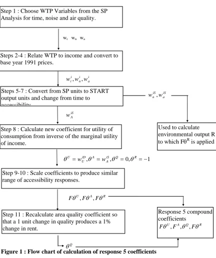
The process for converting the results of the SP survey into the four coefficients used above in DELTA is described in this section in outline only, for further information see appendix A. The results from the SP survey are for specific units and for 1996 prices. The variables produced were not initially related to income, though other variables were produced which reflected the income effect, see Wardman et al (1997). Thus the process for converting from the SP results into the DELTA coefficients involves many steps to take account of changes in units, income effects, difference between time and accessibility, and change of base year between SP survey and START base year. The final steps include a scaling to account for a change in the base utility of consumption coefficient. The outline procedure is as follows :-

Notation used in flow chart :

Willingness to pay values are generally given by the letter w with various subscripts and superscripts. Location model coefficients are denoted by θ with relevant subscripts as in equation 2 above. Note that for simplicity the household subscript h has been dropped.

Thus we have :-

wt willingness to pay for time savings wn willingness to pay for changes in noise wa willingness to pay for changes in air quality

w_ti willingness to pay for time savings by household income i in 1991

w_ni willingness to pay for changes in noise by household income i in 1991

w_ai willingness to pay for changes in air quality by household income i in 1991

wA iS

willingness to pay for accessibility savings by household income i in 1991 related to START units S

wn iS

willingness to pay for changes in noise by household income i in 1991 related to START units S

w_UiD willingness to pay for changes in utility of consumption U by household income i in 1991 related to DELTA units D

θU =

coefficient of response to change in utility of consumption θA =

coefficient of response to change in accessibility θQ ₌

coefficient of response to change in area quality θR =

coefficient of response to change in transport-related environmental quality F is the income related scaling factor which ensures θA is in the same range for

Step 1 : Choose WTP Variables from the SP Analysis for time, noise and air quality.

wt wn wa

w_niS,w_aiS Steps 5-7 : Convert from SP units to START

output units and change from time to accessibility

Steps 2-4 : Relate WTP to income and convert to base year 1991 prices.

w w w_ti n i

a i , ,

w_AiS

Figure 1 : Flow chart of calculation of response 5 coefficients

1. Step 1 : Choose variables from SP results for time (accessibility), noise and air quality.

Values of time, noise and air quality were chosen from the preferred model resulting from the SP analysis. The variables chosen were Car Save for time (accessibility), noise4 for noise and AirLM2 for air quality, taken from Wardman et al (1997). These are wt, wn, and wa in figure 1.

2. Step 2 : Produce relationship to income (1996) for 3 WTP variables. Linear regression produced for 3 variables (see Appendix A)

3. Step 3 : Scale to 1996 weekly incomes by household type. Step 8 : Calculate new coefficient for utility of

consumption from inverse of the marginal utility of income.

Step 9-10 : Scale coefficients to produce similar range of accessibility responses.

θU θ θ θ

U

iD A

A

iS Q R

w w

= , = , =0, =−1

θ , θ , θ F U F A F R

Step 11 : Recalculate area quality coefficient so that a 1 unit change in quality produces a 1% change in rent.

θQ

Response 5 compound coefficients

FθU,FA,θQ,FθR

Used to calculate environmental output R to which FθR

Incomes in base year per household were in location model input files which were then factored to yearly incomes in 1996 to make use of the regression models from step 2.

4. Step 4 : Convert to WTP for base year 1991.

The conversion factor used is based upon START earnings index of 1.8 over

20 years i.e. for converting from 1996 back to 1991 use 1 10298

5

. ⎛

⎝⎜ ⎞⎠⎟ = 0.863. 5. Step 5 : Calculate relationship between accessibility as defined in START

output and changes in in-vehicle-time as used in the SP questionnaire. Derived from START runs (see Appendix A).

6. Change Noise units

Change from percentage changes to perceived dBA changes - factor by 7 (see Appendix A)

7. Change air quality units for CO only (see Appendix A)

8. Calculate new utility of consumption coefficient using program UCML11 Setting inputs as follows θhU

=0, θhQ=0, θhR=-1, and i.e. the accessibility values from the SP model scaled by income for each household and the IVT/accessibility ratio as in steps 1-5. The program then calculates the new coefficient on utility of consumption . This is done by calculating the change in utility of consumption for a 1 unit rise in income and hence the inverse of the marginal utility of income which is equal to the willingness to pay for a 1 unit change in utility of consumption w .

θhA A iS w =

θhU U iD w =

U iD

9. Step 9 : Produce a scaling factor.

The accessibility coefficients derived in steps 1-6 were scaled so that the values were within the previous range i.e. -0.001 to -0.006. This was achieved by forming a linear relationship with household income so that the highest household income had an accessibility coefficient of -0.001 and the lowest household income had an accessibility coefficient of -0.006. This produced household specific scaling factors which were then used in step 10.

10. Step 10 : Scale coefficients The coefficients input in step 8 plus the calculated θhU

are then scaled by the specific factors produced from step 9.

11. Step 11 : Recalculate the area quality coefficient.

This process is the same as for the previous set of coefficients in that it is derived from DELTA runs so that a 1 unit change in quality produces a 1% change in rent.

4.

A comparison of response 1 and response 5 coefficients

This section shows how the coefficients from response 5 are related to household income and how they compare to response 1 coefficients.

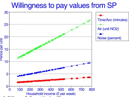
Figure 2 shows the willingness to pay relationships , , and derived from the SP analysis for values of time, air quality and noise versus household income. The coefficients are plotted against household income. Figure 2 shows that from the SP analysis the higher household incomes are willing to pay more than lower household incomes for improvements in noise, time and air quality.

w_ti w_ni w_ai

Figure 3 shows the income related scaling factor derived from the accessibility relationships between R1 and R5 discussed in appendix A and applied to utility of consumption, noise and pollution. This scaling factor is represented by F in the flowchart although it is actually a set of factors related to each households’ income. The area quality coefficient is not scaled by F as it is calculated post-scaling to give a 1% change in rent for a change of 1 unit in area quality. This process results in the set of response 5 coefficients FθhU_{, Fθ}hA_{, θ}hQ _{and Fθ}hR

. (Here it could be argued that the area quality coefficient is equivalent to a scaled coefficient FθhQ

as it was calculated with all others scaled.)

Ideally we would base a comparison on the willingness to pay values for each attribute for response 1 and response 5. However this is not practicable as the two responses were derived using different methods and the willingness to pay for response 1 are not available for noise and accessibility as the analysis resulted in direct θ values rather than willingness to pay. However for air quality we can compare the values for response 1, taken from Tinch (1995) from a Norwegian study; which had a range of £282 - £561 per annum for a 50% reduction in air pollution with those used in response 5 which had a range of £211 - £400 plus calculated from tables 5 and 6 Wardman et al (1997). The willingness to pay appears to be lower in the UK than in Norway (although the income range was different ?).

A further valid comparison is to look at the ratios of the coefficients with the coefficient on utility of consumption i.e. we look at the relative utilities of accessibility, noise, pollution and area quality with respect to willingness to forgo utility of consumption across the responses. This analysis is necessary as the scaling of utility of consumption coefficients has had the effect of changing the relative importance of the responses in terms of overall utility of consumption and therefore of location. Dividing the coefficients through by the coefficient on utility of consumption is a means of expressing the response to changes in accessibility, noise

and pollution in terms of ability to influence changes in rent for example F

F A U θ

Figure 2 : Willingness To Pay variables from SP

Time/Acc (minutes)

Air (unit NO2)

Noise (percent)

Willingness to pay values from SP

0 100 200 300 400 500 600 700 800 Household income (£ per week)

0 5 10 15 20 25 30

Pe

n

ce

p

e

r

u

n

it

Figure 3 : Scaling factor

0 100 200 300 400 500 600 700 800

Household income (£ per week) 0

0.05 0.1 0.15 0.2 0.25 0.3 0.35

Sca

lin

g

f

a

ct

o

r

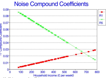
Figures 4-7 show the ratios of coefficients to the coefficient on utility of consumption. Figure 4 shows that the noise1 response relative to rent (or Utility of consumption) for the R5 response is a lot lower than for R1 as income increases.

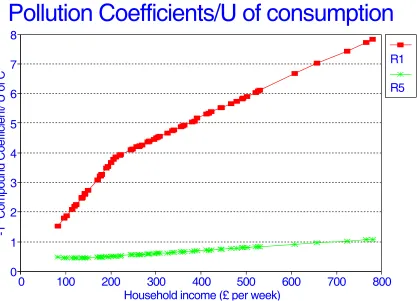
Figure 5 shows that the pollution2 response for R5 has a lower response relative to rent than R1 does. However this pollution response also has the additional complication that for R5 the response is based solely on CO output whereas the R1 response is based upon CO, NOx and VOC’s which may have implications when comparing the coefficients.

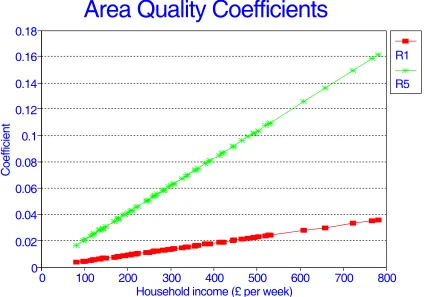
Figure 6 shows the area quality coefficients have the same general curve, as R5 was not factored by the scaling factor, again R5 response relative to rent is actually lower than R1 relative to rent.

Figure 7 shows the accessibility response. High incomes are more responsive relative to rent for both R1 and R5. Again R5 response is lower than R1 which has four curves separated by SEG.

For all four variables the sensitivity to change increases with higher incomes as reflected in the willingness to pay relationships shown in figure 2.

1

Note that for noise the compound response is plotted i.e. for response 5 and for response 1.

F Rw n iS

θ θR

n iS w

2

Note that for pollution the compound response is plotted i.e. for response 5 and for response 1.

F Rwa iS

θ θR

Figure 4 : Noise / Utility of consumption

R1

R5

Noise Coefficients / U of Consumption

0 100 200 300 400 500 600 700 800

Household income (£ per week) 0 1 2 3 4 5 6 7 8 9 10 -1 * C o mp o u n d C o e ff ici e n t/ U o f C

Figure 5 : Pollution / Utility of consumption

R1

R5

Pollution Coefficients/U of consumption

0 100 200 300 400 500 600 700 800

Figure 6 : Area Quality / Utility of consumption

R1

R5

Area Quality / U of consumption

0 100 200 300 400 500 600 700 800

Household income (£ per week) 0

2 4 6 8 10 12 14

C

o

e

ff

ici

e

n

t

/

U

o

f

C

Figure 7: Accessibility / Utility of consumption

R1

R5

Accessibility / U of consumption

0 100 200 300 400 500 600 700 800

Household income (£ per week) 0

0.05 0.1 0.15 0.2 0.25 0.3 0.35

C

o

e

ff

ici

e

n

t

/

U

o

f

Figures 8-12 show the compound coefficients, after scaling, on utility of consumption, accessibility, area quality, noise and pollution against household income (though for the accessibility coefficient it is easy to spot the SEG groupings from R1) for both response 1 and response 5.

4.1 Utility of consumption

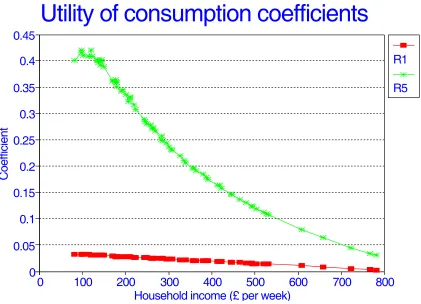
Figure 8 implies that lower income households are more sensitive to changes in rent. Response 5 is greater than response 1 for all incomes and the shape of the curve is characterised by the scaling factor curve in figure 3 above.

4.2 Accessibility

From Figure 9 it can be seen that the assumed linear relationship for R5 used to set the accessibility ranges to those used in R1 gives a completely different set of coefficients compared to R1. This assumption that high income households have a lower response to changes in accessibility forms the basis of the scaling factor curve in figure 3 which is then applied to utility of consumption, noise and pollution coefficients.

The arguments for the assumption are :-

• high income households generally live further from their work place / city centre and so generally accept living in zones with lower accessibility (for reasons such as better quality etc.)

• lower income households cannot afford outer areas and value savings made on transport costs.

This appears at first sight to be contrary to the willingness to pay curve for time savings. However, as figure 7 shows the higher income households are willing to pay more for savings in accessibility relative to changes in utility of consumption.

4.3 Area Quality

Figure 10. Area quality was derived from the R1 estimates and is simply factored by 4.5, this value being obtained from running DELTA so that a 1 unit change in quality causes a 1% change in rent. Higher income households are more responsive to changes in area quality.

4.4 Noise

4.5 Pollution

Figure 12. Again the scaling factor has been applied to the pollution coefficients for R5 and has inverted the WTP relationship in figure 2. The initial R1 curve was a quadratic and so is similar to R5 for high income households but has lower sensitivity for low income households. Again the ratio with utility of consumption shown in figure 5 shows that the response increases with higher incomes though response 5 is far lower than response 1.

Figure 8 : Utility of consumption coefficients

R1

R5

Utility of consumption coefficients

0 100 200 300 400 500 600 700 800

Household income (£ per week) 0

0.05 0.1 0.15 0.2 0.25 0.3 0.35 0.4 0.45

C

o

e

ff

ici

e

n

Figure 9: Accessibility coefficients

R1

R5

Accessibility Coefficients

0 100 200 300 400 500 600 700 800 Household income (£ per week)

0.001 0.0015 0.002 0.0025 0.003 0.0035 0.004 0.0045 0.005 0.0055 0.006

-1

*C

o

e

ff

ici

e

n

t

Figure 10 : Area Quality coefficients

R1

R5

Area Quality Coefficients

0 100 200 300 400 500 600 700 800

Household income (£ per week) 0

0.02 0.04 0.06 0.08 0.1 0.12 0.14 0.16 0.18

C

o

e

ff

ici

e

n

Figure 11 : Noise compound coefficients

R1

R5

Noise Compound Coefficients

0 100 200 300 400 500 600 700 800

Household income (£ per week0 0 0.01 0.02 0.03 0.04 0.05 0.06 0.07 0.08 0.09 -1 * C o mp o u n d C o e ff ici e n t

Figure 12 : Pollution compound coefficients

R1

R5

Pollution Coefficients

0 100 200 300 400 500 600 700 800

Appendix A : Detail of steps used to produce response 5 coefficients

Step 2 : Produce relationship to income in 1996 for 3 chosen variables from step 1.

The regression was calculated using the mid-points of the first five income bands in the SP analysis as the independent variable and dividing the coefficients by the five tax1 variables to produce the dependent Y values. The final income band was ignored in the analysis. Each regression had an R2 value of 0.967.

The following table gives the linear regression results for the three variables :-

Variable Constant X-coeff

Time-Car-Save 0.012972 5.67E-07

Air-LM2 0.095595 4.18E-06

Noise4 0.034403 1.5E-06

The units are as expected so for example for time-car-save an income of £30,000 p.a. gives a value of 0.03 or 3 pence per minute. The units for AirLM2 are pence per unit change in NO2, for noise pence per percentage change.

Step 5 : Calculation of relationship between accessibility and in-vehicle-time

In order to use the coefficients derived from the SP survey for changes in in-vehicle-time it was necessary to derive the relationship between the modelled in-vehicle-in-vehicle-time and the modelled accessibility for changes in certain supply conditions.

It was possible to produce changes in car and bus in-vehicle times together (via speed flow data) with a range of percentage changes between -7% and -35% for zone to zone movements with associated changes in bus in-vehicle times of between -7% and +8% which produces changes in the overall accessibility measure in the range 4 to -7%.

It was possible to change bus in-vehicle time by 3 to 14% with only slight changes in car times which produce less than a 1% change in overall accessibility measures.

The revised method was as follows :-

1. to use 6 START input scenarios for car and bus speed changes (plus an LRT strategy).

2. to produce a zone based average in-vehicle time and hence a change in average in-vehicle time for car, bus and for a composite based on a split of 65% car 35% bus.

3. to produce the ratio by zone:

Ratio Abs Change IVT Household Trip rate Abs Change Accessibility

= . _ * _ _

i.e. change in IVT divided by {absolute change in accessibility for a particular household (from ASRV file) divided by the average household trip rate for that household} for car, bus and composite modes. This is done for household types 10 and 62 which are young single employed SEG 2 and young couple with children (2 employed) SEG 2.

4. to repeat steps 2 and 3 for the set of START scenarios.

5. to average this ratio over the 14 inner zones and by the 25 zones, weighted by population in those zones, for car, bus and composite modes.

6. choose a representative ratio for use in the overall process

Note that in step 2 the averaging process will be a straight average over the time periods and zones of what is currently available. This is a simplification but it allows us to produce a set of coefficients within the time available.

Car and bus coefficients are being developed separately as there are different value of time coefficients and also different changes in the overall accessibility measure when bus changes are implemented alone (see above).

RESULTS Over 14 Zones

The following tables show the ratios (for each household in turn) for car, bus and composite modes for each household over the range of scenarios. The scenarios are described by the expected change in the input in-vehicle time for the car and bus mode, noting that where car is changed the bus speeds also change! The last row of each table is for a run which implemented LRT only, it may not be useful here as the composite times do not include LRT times.

Results for HH10 : Young Single Employed SEG 2 Start Input in terms

of % change in I.V.T

(IVT change * HH trip rate) ÷ Accessibility change

CAR BUS CAR BUS COMPOSITE

-20 0 0.79 0.64 0.74

30 0 0.87 0.72 0.81

-20 20 0.87 0.38 0.70

0 20 0.14 3.11 1.18

0 -20 0.14 3.09 1.17

0 -40 0.14 3.05 1.16

Results for HH62 : Young Couple + children 2 Employed SEG 2 Start Input in terms

of % change in I.V.T

(IVT change * HH trip rate) ÷ Accessibility change

CAR BUS CAR BUS COMPOSITE

-20 0 0.81 0.65 0.75

30 0 0.89 0.73 0.83

-20 20 0.89 0.38 0.71

0 20 0.14 3.13 1.18

0 -20 0.14 3.10 1.18

0 -40 0.14 3.05 1.16

LRT LRT 0.06 0.15 0.09

First of all the ratios do not change between households. However the ratios are generally below 1.0 for car strategies which implies we reduce the value of time coefficient. This was not the expected result as in-vehicle time is only part of the generalised cost and so it was expected that the changes in in-vehicle time would be larger than the associated changes in accessibility. This can be explained by the fact that the changes in accessibility are for the full 25 zones compared to the changes in in-vehicle-time which are for the inner 14 zones only.

The ratios vary according to the strategy implemented, car only strategies giving significantly different results to bus only strategies even at the composite level. Although the LRT ratios are probably not valid the changes in accessibility caused by implementing LRT were a factor of 10 greater than those for car only strategies.

Results over 25 zones

The same method was applied for the young single employed SEG 2 household for all 25 zones. The results are shown in the following table.

Results for HH10 : Young Single Employed SEG 2 over 25 zones Start Input in terms of

% change in I.V.T

(IVT change * HH trip rate) ÷ Accessibility change

CAR BUS CAR BUS COMPOSITE

-20 0 1.48 1.4 1.45

30 0 1.48 1.4 1.45

-20 20 1.54 0.56 1.2

0 20 1.18 163.8 58.1

0 -20 0.25 5.41 2.05

0 -40 -0.02 -19.36 -6.79

Further problems arise for bus only strategies in that the car ratio can fall below 1.0, the bus ratio can be dominated by outer zones which have only a small change in accessibility (hence high ratio) and for some outer zones the change in accessibility was small and of the wrong sign giving a negative ratio! These effects can also feed through to the composite ratio.

The choice of ratio was determined by the fact that the DELTA model responds to composite changes in accessibility and could not be broken down by mode. It was decided that a value between the bus strategy value over 14 zones (1.18) and the car strategy value over 25 zones (1.45) should be used. The value chosen was 1.3.

Step 6 : Change Noise units from percentage change to change in dBA.

The willingness to pay for percentage changes in noise must be factored to take account of the START output which is given as changes in dBA for each zone. The factor for a percentage change was considered as follows :-

We have two assumptions to consider in respect to what a halving or doubling of noise actually meant to respondents. The first is to assume the change to be actual change in energy, the second is to assume a perceived change. The first assumption implies a change of 3 dBA to double or halve energy or noise intensity. The second assumption on perceived change is to say that a 10 dBA change is equivalent to a halving or doubling of the noise level.

Method 1

Energy : Consider a noise level L100 for noise intensity I. Then to find the value of a 1 dBA increase we form the following equations :-

L100 = 10 Log10(I)

L100+x = 10 Log10[(I)*(100+x)/100]

L100+x = L100 + 10 Log10[(100+x)/100]

thus for a 1 dBA change we need to solve 1 = 10 Log10[(100+x)/100] which gives x=26 i.e. a 26% increase in noise level is equivalent to a 1 dBA increase or L126. For a 1 dBA decrease then x = -21% or L79

Similarly we have 3 dBA increase is equivalent to a 100% increase and 3 dBA decrease is equivalent to a 50% decrease in noise level i.e. L200 and L50 respectively.

26 100 100

* ( *N)

where N is for a 1% change. This equals a factor of 26 for increases

in noise and similarly 21 for a decrease in noise.

Perception : Method 2

This method uses the same equations as the previous method but actually solves the problem for any value of change in dBA say G.

For energy assumption we simply solve :-

x = ALog ⎛G

⎝⎜ ⎞⎠⎟− 100

10 100

10 (1)

For the perception model we require a change of +10 dBA to give a 100% increase in perceived level of noise or

(

)

100=100ALog₁₀ 10*f −100

−

(2)

which gives a value for f of 0.03. We then have a similar equation for perception as for energy :-

(

)

x_p =100ALog₁₀ G* .0 03 100 (3)

where xp is the percentage change in perceived noise level.

Solving equation 1 and 3 for various changes in dBA G we form the following table of results :-

G =Change in dBA of noise level

x =

percentage change in intensity

xp = perceived percentage change

-10 -90 -50

-5 -68 -29

-3 -50 -19

-2 -37 -13

-1 -21 -7

+1 26 7

+2 58 15

+3 100 23

+5 216 41

+10 900 100

This method gives the same perceived percentage change for a 1 dBA increase as for decrease, i.e. 7% implying a factor of 7 to be applied to the noise4 value which is then applied to the noise output from START.

Step 7 : Change air quality units to account for START outputs CO, NOX and VOC.

quality willingness to pay coefficient (based on NO2 measurements) was to be plit between the START pollutants by the same weights as used in the initial analysis

ut calculations which confirm the ranges of measured NO2 (micro-rammes /m3) to be in line with the ranges of CO output by START in ppm. The

lues measured as weekly averages in micro-grammes per m .

5 - 29.27 ppb weekly average

ile hour NO2)

/24 DMRB to factor by 4 to give NOX from NO2 50 - 300 ppb NOX verage during traffic peak hour.

km/h from START output and using the relative mission graph from old TRRL (REF?) model to factor NOX to CO emissions divide

hourly value gives 2.3 - 8.59 pm CO 8 hour maximums.

are higher for some reason.

ns then to get from 11 to 2.3 would imply a factor of .209, whereas to get from 56 to 8.59 would imply a factor of 0.15 i.e. no common

it with the measured range en we have 2/11=0.18 and 10/56=0.18.

n CO output factored by 5.6 (the inverse of 0.18). The model is set up to factor the outputs for pollution rather than factor the The air

s

i.e. derived from relative toxicity and Tinch’s tables. However the START output for NOX did not lie within the range implied by the NO2 measurements and so an alternative was to associate the willingness to pay from NO2 to the START output CO measured in ppm.

This section sets o g

assumptions are taken from the Design Manual for Roads and Bridges Volume 11 unless otherwise stated.

Starting with the NO2 va 3

We collected the range 11 - 56 micro-grammes/m3.

Divide through by 1.913 to convert to ppb giving 5.7

Multiply by 2.4 to give 98th percentile 1 hour NO2 13.8 - 70.25 ppb (98th percent 1

Graph page 6 a

Assuming average speed of 45 e

by 0.075 giving 666 - 4000 ppb CO peak hour average.

Convert to maximum 8 hourly average using 1.19+1.85* p

The START outputs a range of 2 to 10 ppm CO 8 hour maximums with 8.3 and 8.9 in the centre. Zones 15 and 16

Producing a common factor.

If we take the above calculatio 0

factor due to the very last step with the intercept of 1.19.

However if we take the START CO range and compare th

coefficient. The other pollutants will be factored by zero to eliminate them from the response.

Step 8 : Calculate new utility of consumption coefficient using program UCML11.

θhU _θhQ _θhR = iS

T/accessibility ratio as in steps 1-5. The program then calculates the new

R

h =θUh h +θAh h +θRh h

the form

P

h Uh h Ah

i h Nh i ph i p p = + + +

Setting inputs as follows =0, =0, =-1, and w i.e. the accessibility _A values from the SP model scaled by income for each household and the

θhA

IV

coefficient on utility of consumptionθhU =w_UiD. This is done by calculating the change in utility of consumption for a 1 unit rise in income and hence the inverse of the marginal utility of income which is equal to the willingness to pay for a 1 unit change in utility of consumption wU

iD .

The UCML11 program also calculated

V_i U_i A_{i i}

in

V_i θ U_i θ A φ N

∑

here

is the utility of location in zone i for household type h

is the utility of consumption for households h in zone I

ouseholds h

Ni φNh φPh

r household type h θR

ironment respectively

ts are household type h, residential oorspace in zone i and utility of location

ho types (check with David). This set of oefficients was to be used in step 10 to re-scale the coefficients on accessibility and w

V_ih

U_ih

A_ih is the accessibility of zone i for households h

R_ih is the transport related environmental output for zone i h

P_ip is the components p of air pollution at I (from START) is the noise level at i (from START)

WTP of households h for reduction in Ni WTP of households h for reduction in P_ip θUh

is the (marginal utility of income)-1 fo θAh

, h are WTP for accessibility and env

The inputs for the program were derived in steps 1-7. The outpu

h, zone i, number of households choosing to locate in zone i of type

fl V_ih.

The cross-sectional analysis of this data set will produce a set of coefficients for V_ih perhaps grouped by income bands or house ld

c

Step 11 : Recalculate the area quality coefficient.

The base DELTA model is run with the new coefficients for all except area quality a typical zone is then The area quality coefficients are djusted in an iterative manner until an adjustment of 1 unit causes approximately a

inch, R (1995). The valuation of environmental externalities. Report prepared for nt of Transport

(previous values are first used for area quality). The quality of increased by 1 unit and the model is run again.

a

1% change in rent for the zone considered. The process is applied to three or four zones to give a better overall result. The resulting factor of 4.5 was applied to all the previous area quality coefficients.

Reference

T