Article
MPC for LPV Systems Based on Parameter-Dependent
Lyapunov Function with Perturbation on Control Input
Strategy
Pornchai Bumroongsri
and Soorathep Kheawhom
*Department of Chemical Engineering, Faculty of Engineering, Chulalongkorn University, Phayathai Rd., Patumwan, Bangkok 10330, Thailand
E-mail: [email protected]*
Abstract. In this paper, the model predictive control (MPC) algorithm for linear parameter varying (LPV) systems is proposed. The proposed algorithm consists of two steps. The first step is derived by using parameter-dependent Lyapunov function and the second step is derived by using the perturbation on control input strategy. In order to achieve good control performance, the bounds on the rate of variation of the parameters are taken into account in the controller synthesis. An overall algorithm is proved to guarantee robust stability. The controller design is illustrated with two case studies of continuous stirred-tank reactors. Comparisons with other MPC algorithms for LPV systems have been undertaken. The results show that the proposed algorithm can achieve better control performance.
Keywords: MPC, LPV, parameter-dependent Lyapunov function, perturbation on control input strategy, continuous stirred-tank reactor.
ENGINEERING JOURNAL Volume 16 Issue 2 Received 14 October 2011
Accepted 21 December 2011 Published 1 April 2012
1.
Introduction
Model predictive control (MPC) is an effective control algorithm widely used in the chemical processes. At each sampling time, MPC uses an explicit process model to solve an open-loop optimization problem and implements only the first element of input sequence. Model predictive controllers based on linear models are typically used. This is because the on-line optimization problem can be formulated as the convex optimization problem by either linear programming or quadratic programming [1]. This is a good assumption for typical processes. However, most of the chemical processes are nonlinear. Thus, when the operating conditions undergo significant changes, the performance of linear MPC can deteriorate drastically. Moreover, the stability of the control system cannot be guaranteed.
In [1], min-max predictive control strategy was presented. The nonlinear system is approximated by the polytopic uncertain system. The goal is to design a state feedback control law which minimizes the upper bound on the worst-case performance cost. The optimization problem at each time step is formulated as the convex optimization problem involving linear matrix inequalities. The algorithm is proved to guarantee robust stability. However, the algorithm turns out to be very conservative. This is due to the fact that the nonlinear system is approximated by the polytopic uncertain system. Moreover, the scheduling parameter is not taken into account in the controller synthesis.
In order to reduce the conservativeness, the idea of controlling nonlinear systems by using linear parameter varying (LPV) systems has been widely investigated. At each sampling instant, the scheduling parameter is measured on-line. However, its future behaviour is considered to be uncertain and varying within the polytope. In [2], Quasi-min-max MPC algorithm for LPV systems was presented. The control input is computed by minimizing the upper bound on the quasi-worst-case performance cost. The algorithm is seen as an extension of the algorithm presented in [1] by keeping the first control input as a free decision variable. The algorithm is proved to guarantee robust stability. However, an invariant ellipsoid constructed to guarantee robust stability is derived by using a single Lyapunov function. Thus, the conservative result is still obtained.
A feedback min-max MPC algorithm for LPV systems subject to bounded rates of change of parameters was presented in [3]. The algorithm in [2], where open-loop MPC scheme is limited to one step control horizon, is extended to the general case of control horizon of arbitrary length N. The bounded parameter variations are assumed to be known. Moreover, they are exploited in the controller synthesis in order to improve control performance. However, the stability of the control system cannot be guaranteed. This is due to the fact that the constraint on terminal invariant set is not explicitly imposed. Moreover, input and output constraints satisfaction before switching horizon N cannot be guaranteed as pointed out in [4].
The ability of on-line MPC is limited to relatively slow dynamics processes. In order to reduce on-line computational demand, a number of researchers have begun to study off-line MPC. In [5], an off-line formulation of MPC using linear matrix inequalities was presented. A sequence of explicit control laws corresponding to a sequence of invariant ellipsoids is constructed off-line by solving the optimization problem presented in [1]. At each sampling time, the smallest ellipsoid containing the measured state is determined and the real-time control law is calculated by linear interpolation between control laws of two adjacent invariant ellipsoids. The stability of the control system is proved to be guaranteed. However, the conservative result is obtained. This is due to the fact that the algorithm directly solves off-line the optimization problem presented in [1]. In [6], an ellipsoidal off-line MPC algorithm based on nominal performance cost was presented. The algorithm directly extends the algorithm presented in [5] by choosing the nominal performance cost to substitute the worst-case performance cost.
From the preceding review, we can see that robust stability is usually achieved with conservative result. In this paper, the closed-loop MPC strategy for LPV systems is developed. The proposed algorithm consists of two steps. The first step is derived by using parameter dependent Lyapunov function [7] and the second step is derived by using the perturbation on control input strategy [3, 8]. The scheduling parameter and the bounded parameter variations are taken into account in the controller synthesis. Thus, the control performance is improved.
Notation: For a matrixA, T
A denotes its transpose, 1
A denotes its inverse. I denotes the identity matrix.
For a vectorx, x(k/k)denotes the state measured at real timek, x(ki/k) denotes the state at prediction time ki predicted at real timek. The symbol denotes the corresponding transpose of the lower block
part of symmetric matrices.
Kki(
x
(
k
))
Co
{
K(
p
ki1)
x
(
k
)}
denotes the closed convex hull of alli
-steps state trajectories fromx
at timek
under the state feedback gainK
.vert
{
Kk i(
x
(
k
))}
denotes allvertices of Kk i
(
x
(
k
))
. The matrix inequalityA
B
(
A
B
)
means thatA
andB
are square symmetric andA
B
is positive (semi-) definite.2.
Problem description
The model considered here is the following discrete-time LPV system:
) ( ) ( ) ( ) ( )) ( ( ) 1 ( k Cx k y k Bu k x k p A k x (1) where x(k) is the state of the plant, u(k)is the control input and y(k) is the plant output. We assume that the scheduling parameterp(k) is measurable on-line at each sampling timek. Moreover, we assume that
Ω k p
A( ( )) , ΩCo{A1,A2,...,AL} (2)
where Ω is the polytope, Codenotes convex hull, Ajare vertices of the convex hull and
L
is the number of vertices of the convex hull. Any A(p(k)) within the polytope Ω is a linear combination of the vertices such that j L j j A k p k pA
1 ) ( )) ( ( 1 ) ( 0 , 1 ) ( 1
p k pj k
L j j (3) Further, let )} ( ) ( { )) (
(xk Co K pk i 1 xk i k K (4)
denote the closed convex hull of all
i
-steps state trajectories fromx
at timek
under the state-feedback gainK
whereBK k p A k p
K
( ( )) ( ( )) (5)
)) 1 ( ( ))... 2 ( ( )) 1 ( ( )) ( ( )
( 1
K pki K pk K pk K pk K pk i (6)
Following [8], the above sets can be computed according to
}
)
1
(
))},
(
(
{
,
{
))
(
(
( ( 1)) 1P
κi1
i
k
p
k
x
vert
z
z
Co
k
x
K Kk ii k
K pk i
}} ) ( {
{co p k p
vert 1 κ P }} ) 1 ( { {
2 vert co pk p
κ P }} ) 2 ( {
{co pk i p
vert
i 1 κ
P
(7)
where
p
is the bounded parameter variation and it is assumed to be known. The aim of this research is to find a state feedback regulation)) ( ( )
(k g xk
u (8)
which stabilizes Eq. (1)-(3) and achieves the following performance cost ) ( max min 0 , )) ( ( ) /
(k i k Apk i i J k
u
) / ( ) / ( 0 0 ) / ( ) / ( ) (0 u k i k
where
0
andR
0
are symmetric weighting matrices, subject to constraints max , ) / ( hh k i k u
u ,h1,2,3...nu (10)
max ,
) /
( r
r k i k y
y , r1,2,3...ny (11)
In [1], the optimization problem Eq. (9) is formulated as the convex optimization problem involving linear matrix inequalities. The goal is to design the state feedback control law which minimizes the upper bound on the worst-case performance cost. The algorithm is derived by using a single Lyapunov function. Consequently, this approach turns out to be conservative. In order to reduce the conservativeness, MPC synthesis by using a parameter-dependent Lyapunov function is developed.
Lemma 2.1: Consider the LPV system (1) at each sampling time
k
, the state feedback control law which minimizes the upper bound
on the worst-case MPC objective J(k) and asymptotically stabilizes the closed-loop system within aninvariant ellipsoid
L j j j T Q k p Q x Q x x 1 1 ) ( , 1 / is given by u(ki/k)K(p(ki))x(ki/k),
1 1 , ) ( )) (
( j j -j
L
j
j
j k i K K YG
p i
k p
K
where
Y
j,G
j andQ
jare the matrix variables obtained by solving the following problem:min
j j j
γ,Y ,G ,Q
γ
L , j , Q x(k/k) x(k/k) j T ... 2 1 0 1 s.t. (12) 1 2 1 2
0 1 2... 1 2... 0
0 0
T j j j
j j j l
j
j
G G Q
A G BY Q
, j , L, l , L
Θ G γI
R Y γI
(13) ... 2 1 ... 2 1 0 2 max u h, hh j T j j T j n , , h u L, X . , j , Q G G Y X (14) ... 2 1 ... 2 1 0 2 max y r, rr j T j j T T j j j n , r , y L, S , j , Q G G C ) BY G (A S (15)
Proof. Proof details can be found in [7].
The existence of a symmetric matrix
X
withX
hh
u
h2,max,
h
1
,
2
,..
n
u,
such that, 0 j T j j
T G G Q
Y X
L
j
1
,
2
,...
guarantees thatu
h(
k
i
/
k
)
u
h,max and the existence of asymmetric matrix
S
withS
rry
r,
r
1
,
2
,..
n
y2 max
,
such that
0
j T j j T T j jj
G
BY
)
C
G
G
Q
(A
S
,
L
j
1
,
2
,...
guarantees thaty
r(
k
i
/
k
)
y
r,max. For more details, the reader is referred to [9].
)
(k N
x . Moreover, the input and output constraints satisfaction before switching horizon N cannot
be guaranteed [4]. In the following lemma, we will present the perturbation on control input strategy which can ensure robust stability and robust constraint satisfaction.
Lemma 2.2: Given the state feedback gain
K
which asymptotically stabilizes the system (1) within an invariant ellipsoid
/
1
1
x
Q
x
x
T
and satisfies (10), (11), we can ensure that the system (1) is robustly stabilized and (10), (11) are satisfiedby the sequence of control inputs
N
i
k
i
k
Kx
N
i
k
i
k
c
k
i
k
Kx
k
i
k
u
h h h
,
))
/
(
(
1
,....
1
,
0
,
))
/
(
)
/
(
(
)
/
(
(16)if there exists a sequence of free control inputs
(
/
)
01
Ni
k
i
k
c
satisfying the following inequalities:
χ
(x(k))
vert
k)
N
z(k
,
k
N
k
z
Q
k
N
k
z
(
/
)
T 1(
/
)
1
/
KkN (17)
,
....N
,
z(k
i
k)
vert
χ
(x(k))
h
,
,....N
,
i
,
u
i/k))
c(k
i/k)
(Kz(k
i k K u
h, h
/
2
1
1
1
0
max
(18)
,
....N
,
z(k
i
k)
vert
χ
(x(k))
r
,....N
,
i
,
y
i/k))
(Cz(k
i k K y
r, r
/
2
1
,
1
1
0
max
(19)
Proof. The satisfaction of (17) ensures that
x
(
k
N
/
k
)
,
x
(
k
N
/
k
)
KkN(
x
(
k
))
. If
/
)
(
k
N
k
x
, the state feedback gainK
is able to steer the state fromx
(
k
N
/
k
)
to the origin. Thus, the closed-loop system is robustly stabilized.The satisfaction of (18) ensures that
(Kx(k
i/k)
c(k
i/k))
h
u
h,max,
x(k
i
k)
χ
k i(x(k))
K
/
.Thus, (10) must be satisfied. The satisfaction of (19) ensures that
(Cx(k
i/k))
r
y
r,max,
(x(k))
χ
k)
i
x(k
k iK
/
. Thus, (11) must be satisfied.3.
The proposed MPC algorithm for LPV systems
In this section, the MPC algorithm for LPV systems is proposed. Lemmas 1 and 2 will be used in the controller synthesis. The proposed algorithm consists of two steps. In the first step, the state feedback control law is calculated by using parameter-dependent Lyapunov function. The state feedback control law provided by the first step is designed to robustly stabilize the closed-loop system. In the second step, the state feedback control law calculated from step 1 is perturbed by using a sequence of free control inputs
10
)
/
(
k
i
k
Nic
. The control performance is improved by minimizing an additional performance cost over a perturbation horizon N. The scheduling parameter and the bounds on the rate of variation of the parameters are taken into account in the problem formulation.Algorithm 3.1
Step 1:
At any sampling time
k
, measurex
(
k
)
and find 1,
K
j
Y
jG
j
and
Q
jby solving the optimizationproblem in Lemma 2.1 [7]. Step 2:
Given 1
,
K
j
Y
jG
j
and
Q
j from step 1,a sequence of free control inputs
1 0
)
/
(
k
i
k
iNc
is
N i i C Ji 0, o p t 0J
min
χ (x(k))
vert k) N z(k L , , j , Q γ k) N z(k
J k N
K j -N / ... 2 1 0 / s.t. 1 (20)
γ
J
N
(21)
,
N
,
z(k
i
k)
vert
χ
(x(k))
h
,
N
,
i
,
u
i/k))
c(k
i/k)
z(k
(K
i k K u h, h j
/
...
2
1
1
...
1
0
max (22)
,
....N
,
z(k
i
k)
vert
χ
(x(k))
r
,....N
,
i
,
y
i/k))
(Cz(k
i k K y r, r
/
2
1
,
1
1
0
max (23)
,
,....N
,
z(k
i
k)
vert
χ
(x(k))
i
I
J
i/k)
c(k
R
I
J
i/k)
z(k
Θ
I
i k K n i n i u x
/
1
1
0
0
0
2 1 2 1 (24)Feed the plant by
1
( ) ( ( )) ( ) ( ), ( ( )) ( ) . L
j j j
u k K p k x k c k K p k p k K
The stability of the control system is proved to be guaranteed in Theorem 3.1.
Theorem 3.1: The control law provided by the algorithm 3.1 assures robust stability to the closed-loop system.
Proof. We prove this theorem in two steps. In step a, we prove that the control law i G Y K K i k p i k p K k i k x i k p K k i k u -j j j L j j
j( ) , , 0
)) ( ( ), / ( )) ( ( ) / ( 1 1
provided by step 1 asymptotically stabilizes the closed-loop system. In step b, we prove that by using the perturbations of
10
) / (ki k iN
c to improve control performance, the control law
N i k i k x i k p K N i k i k c k i k x i k p K k i k u ), / ( )) ( ( 1 ,.... 1 , 0 ), / ( ) / ( )) ( ( ) / ( (25)
provided by step 2 asymptotically stabilizes the closed-loop system.
Step a) The proof is based on the same rationale used for proving in Lemma 2.1. Thus, the control law
) / ( )) ( ( ) /
(k i k K p k i xk i k
u provided by step 1 asymptotically stabilizes the closed-loop system.
Step b) By applying Schur complement to (20), with (21), we obtain
N T J k N k z Q k N k
z( / ) 1 ( / ) where
L
j
j j k Q
p Q
1
. )
( This is equivalent to ( / ) 1 ( / )1,
k N k z Q k N k
z T z(k N/k) vert
χk N(x(k))
.K
Thus, the
state x(kN/k) is restricted to lie in an invariant ellipsoid
x/xTQ1x1
and the control lawN i k i k x i k p K k i k
4.
Examples
In this section, we present two examples that illustrate the implementation of the proposed MPC algorithm. For both examples, the numerical simulations have been performed in Intel Core i-5 (2.4 GHz), 2 GB RAM, using SeDuMi [10] and YALMIP [11] within Matlab R2008a environment.
Example 4.1: Consider the following nonlinear model for CSTR where the consecutive reaction
C B
A takes place [12]
2 2 2 2 1 1 2 .
1 1 1 1 .
x Da x x Da x
u x Da x x
(26)
where x1denotes the dimensionless concentration ofA,x2denotes the dimensionless concentration of B,
The control variable u corresponds to the inlet concentration of A. The operating parameters are shown in Table 1. It is assumed that
A
B
is a first order chemical reaction whereasB
C
is a second order chemical reaction.Table 1. The operating parameters of nonlinear CSTR in example 4.1.
Parameter Value
1
Da 1
2
Da 2
By defining the deviation variables x1x1x1,eq, x2 x2 x2,eq, uuueq where
the subscript
eq
is used to denote the corresponding variable at equilibrium condition, we have that all the solutions of (26) are also the solutions of the following differential inclusion0
1
2 1 2
1 2 .
1 .
u x
x p x
x
j j
j
(27)
where jis given by
, 1
0 1
min , 2 2 1
1
1
x Da Da
Da
max , 2 2 1
1 2
1 0 1
x Da Da
Da
(28)
Considerx2,minx2x2,max, the parameter
p
1is given bymin , 2 max , 2
2 max , 2 1
x
x
x
x
p
and the parameterp
2is givenby
min , 2 max , 2
min , 2 2 2
x
x
x
x
p
. In this example, we have two controlled variables x1,x
2and one manipulatedvariable
u
. The objective is to regulate x1andx
2 from 0.05 and 0.1 respectively to the origin bymanipulating
u
. The input and output constraints are given as follows:5 . 2
2 x
2
2 1
u x
[image:7.595.64.524.332.741.2]The discrete-time model is obtained by discretizing (27) using Euler discretization method with sampling time of 0.1 min and it is omitted here for brevity. Here J(k)is given by (9) with 10Iand
. 01 . 0
R It is assumed that pj(k1)pj(k)0.1.
The proposed MPC algorithm will be compared with the MPC algorithms of Kothare et al. [1], Lu et al.
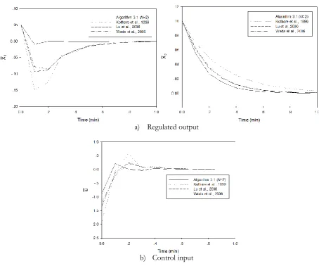
[2] and Wada et al. [7]. Figure 1 shows the closed-loop responses of the system. It can be observed from the figure that the proposed algorithm can achieve less conservative result as compared with other MPC algorithms.
a) Regulated output
b) Control input Fig. 1. The closed-loop responses of nonlinear CSTR in example 4.1.
In [1], the state feedback control law is designed by minimizing the upper bound on the worst-case performance cost. The quadratic function of the state is forced to decrease at each prediction time by the amount of the worst-case performance cost. However, the algorithm turns out to be very conservative. This is due to the fact that the nonlinear system is approximated by the polytopic uncertain system. Moreover, the scheduling parameter is considered to be uncertain and it is not taken into account in the controller synthesis.
In [2], the control input is computed by minimizing the upper bound on the quasi-worst-case performance cost. The algorithm is seen as an extension of the algorithm presented in [1] by keeping the first control input as a free decision variable. The scheduling parameter is measured on-line and it is incorporated into the problem formulation. However, an invariant ellipsoid constructed to guarantee robust stability is derived by using a single Lyapunov function. Thus, the conservative result is obtained.
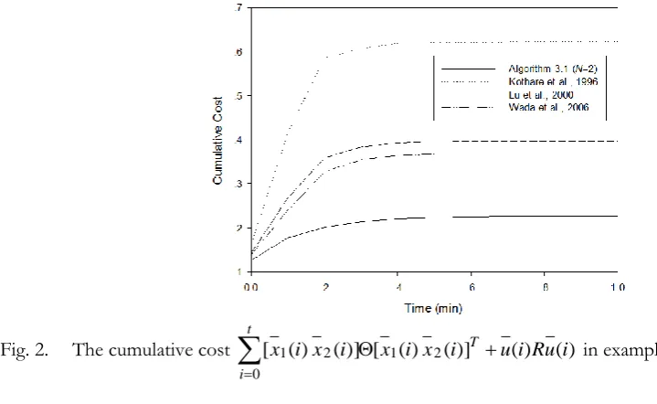
[image:8.595.69.524.184.562.2]Figure 2 shows the cumulative cost
t
i
T u i Ru i
i x i x i x i x
0
2 1 2
1() ()] [ () ()] () ()
[ . It can be observed
that the proposed algorithm gives the lowest cost value as compared to MPC algorithms of Kothare et al.
[1], Lu et al. [2] and Wada et al. [7].
Fig. 2. The cumulative cost
t
i
T u i Ru i
i x i x i x i x
0
2 1 2
1() ()] [ () ()] () ()
[ in example 4.1.
Though the proposed algorithm can achieve less conservative result as compared with other MPC algorithms, it requires higher on-line computational time as shown in Table 2.
Table 2. The on-line computational time in example 4.1.
Algorithm CPU time per step
Algorithm 3.1 Step 1 = 0.196 s
N=2 Step 2 = 0.153 s
Kothare et al. 0.142 s
Lu et al. 0.157 s
Wada et al. 0.196 s
Example 4.2: Consider the following nonlinear model for CSTR where the exothermic reaction AB
takes place [13].
) ( )
(
)
(
. .
T T C V
UA C e k C
H T
T V
q T
C e k C C V
q C
c p A RT Ea o p f
A RT Ea o A AF A
(30)
where CAdenotes the concentration of A in the reactor, T denotes the reactor temperature and Tc denotes
[image:9.595.68.428.152.373.2] [image:9.595.170.425.461.555.2]Table 3. The operating parameters of nonlinear CSTR in example 4.2.
Parameter Value Unit
q 100 l/min
f
T 350 K
AF
C 1 mol/l
V
100 l
1,000 g/lp
C 0.239 J/g K
H
-5x10⁴ J/mol
R
E
a/
8,750 Ko
k
7.2x10¹⁰ min-1UA
5x10⁴ J/min KBy defining the deviation variables CACACA,eq, T TTeq,TcTcTc ,eq where
the subscript
eq
isused to denote the corresponding variable at equilibrium condition, we have that all the solutions of (30) are also the solutions of the following differential inclusion
0 c 2 1 . . T C V UA T C p T C p A j j j A
(31)
where jis given by
, 0 min min 1 p RT Ea o p RT E o C V UA V q e k C H V q e k a p RT Ea o p RT E o C V UA V q e k C H V q e k a max max 0 2 (32)
Consider TminTTmax, the parameterp1is given by
min max max 1 RT E RT E RT E RT E a a a a e e e e
p and the parameter p2is
given by
min max min 2 RT E RT E RT E RT E a a a a e e e e
p . In this example, we have two controlled variables CA, T and one
manipulated variableTc.The objective is to regulate CA and T from 0.2 and 0.5 respectively to the origin
by manipulatingTc. The input and output constraints are given as follows:
K 50 K 50 T mol/l 5 . 0 c A T C (33)
The discrete-time model is obtained by discretizing (31) using Euler discretization method with sampling time of 0.01 min and it is omitted here for brevity. Here J(k)is given by (9) with Iand
. 01 . 0
[image:10.595.194.403.128.305.2]R It is assumed that pj(k1)pj(k)0.1.
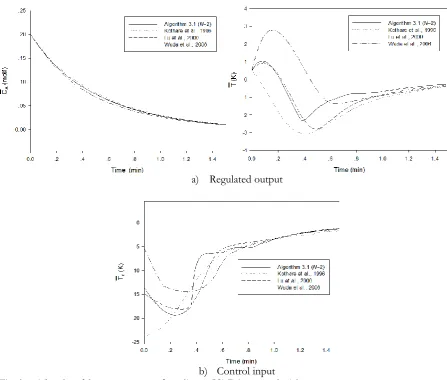
[image:10.595.60.530.335.642.2]a) Regulated output
b) Control input Fig. 3. The closed-loop responses of nonlinear CSTR in example 4.2.
Figure 4 shows the cumulative cost
t
i
c c T A
A i T i C i T i T i RT i
C 0
) ( ) ( )] ( ) ( [ )] ( ) (
[ . It can be observed
from the figure that the proposed algorithm can achieve better control performance as compared to MPC algorithms of Kothare et al. [1], Lu et al. [2] and Wada et al. [7].
Fig. 4. The cumulative cost
t i
c c T A
A
i
T
i
C
i
T
i
T
i
R
T
i
C
0
)
(
)
(
)]
(
)
(
[
)]
(
)
(
[image:11.595.69.517.86.466.2] [image:11.595.66.475.542.754.2]5.
Conclusions
In this paper, the synthesis approach to MPC for LPV systems using linear matrix inequalities is developed. The proposed algorithm consists of two steps. The first step is derived by using parameter dependent Lyapunov function and the second step is derived by using the perturbation on control input strategy. The bounds on the rate of variation of the parameters are taken into account in the controller synthesis in order to improve control performance. The controller design is illustrated with two examples in chemical processes. Comparisons with other MPC algorithms have been undertaken. The results show that the proposed algorithm can achieve better control performance.
Acknowledgement
The authors gratefully acknowledge the financial support provided by the Higher Education Research Promotion and National Research University Project of Thailand, Office of the Higher Education Commission (EN636A).
References
[1] M.V. Kothare, V. Balakrishnan, and M. Morari, “Robust constrained model predictive control using linear matrix inequalities,” Automatica, vol. 32, pp. 1361-1379, 1996.
[2] Y. Lu and Y. Arkun, “Quasi-min-max MPC algorithms for LPV systems,” Automatica, vol. 36, pp. 527-540, 2000.
[3] A. Casavola, D. Famularo, and G. Franze, “A feedback min-max MPC algorithm for LPV systems subject to bounded rates of change of parameters,” IEEE T. Automat. Contr., vol. 47, pp. 1147-1152, 2002.
[4] B. Ding and B. Huang, “Comments on a feedback min-max MPC algorithm for LPV systems subject to bounded rates of change of parameters,” IEEE T. Automat. Contr., vol. 52, pp. 970, 2007.
[5] Z. Wan and M.V. Kothare, “An efficient off-line formulation of robust model predictive control using linear matrix inequalities,” Automatica, vol. 39, pp. 837-846, 2003.
[6] B. Ding, Y. Xi, M. T. Cychowski, and T. O. Mahony, “Improving off-line approach to robust MPC based-on nominal performance cost,” Automatica, vol. 43, pp. 158-163, 2007.
[7] N. Wada, K. Saito, and M. Saeki, “Model predictive control for linear parameter varying systems using parameter dependent lyapunov function,” IEEE T. Circuits Syst., vol.53, pp. 1446-1450, 2006.
[8] A. Casavola, D. Famularo, G. Franze, “Predictive control of constrained nonlinear systems via LPV linear embeddings,” Int. J. Robust Nonlin., vol. 13, pp. 281-294, 2003.
[9] F. A. Cuzzola, J. C. Geromel, and M. Morari, “An improved approach for constrained robust model predictive control,” Automatica, vol. 38, pp. 1183-1189, 2002.
[10] J. F. Sturm, “
Using Sedumi 1.02, a MATLAB toolbox for optimization over symmetric cones
,”Optim. Method Softw.
, vol. 11, pp. 625-653, 1999.[11] J. Löfberg, “YALMIP : A toolbox for modelling and optimization in MATLAB,” in Proceedings of the 2004 IEEE international symposium on computer aided control systems design, Taipei, Taiwan, 2004, pp. 284-289.
[12] J. P. García-Sandoval, V. González-Álvarez, B. Castillo-Toledo, and C. Pelayo-Ortiz “Robust discrete control of nonlinear processes: Application to chemical reactors,” Comput. Chem. Eng., vol. 32, pp. 3246-3253, 2008.