Helicon Wave Propagation in Low Diverging Magnetic Fields.

(1)

Diverging Magnetic Fields

Trevor Alain Lafleur

A thesis submitted for the degree of Doctor of Philosophy

of The Australian National University

(2)

Declaration

This thesis is an account of research undertaken between March 2008 and May 2011 at The Research School of Physics and Engineering, College of Physical and Mathematical Sciences, The Australian National University, Canberra, Australia. Except where ac-knowledged in the customary manner, the material presented in this thesis is, to the best of my knowledge, original and has not been submitted in whole or part for a degree in any university.

(3)

Foremost I would like to thank Rod and Christine for giving me the opportunity to come to Australia and work with them in their lab, especially since I knew almost no plasma physics when I started! Rod is very knowledgeable on a huge range of plasma physics areas, and he blurs the student-supervisor relationship; acting more like a friend than some surly old professor. I appreciate the many discussions we had over the years, and the keen interest you showed in all aspects of the thesis. Thank you also for helping to improve the thesis with many useful suggestions. Many thanks to Christine for showing me the ins and outs of the lab, and for always having time to proof-read reports and manuscripts, and to discuss my many ideas, even when our conversations went on for hours! I admire your patience and dedication to your work, and with your vision and drive you can really inspire those around you. I also appreciate the informal music lessons you gave and for introducing me to Jazz!

A huge thanks to Cormac for always having the time to discuss ideas and helping me in the lab. You really made settling into the group easier, and were responsible for assisting me in finding accommodation during the “drought” when I arrived. I am also very grateful to you for proof-reading my thesis in such detail, and your invaluable suggestions to improve it. You are so easy to get along with, and have the most amazing ability when it comes to knowing what papers are around, even on plasma topics you might not be an expert in. I can directly connect my progress on this thesis to one such paper suggestion that helped me think of a solution I might not otherwise have found.

A project rarely succeeds without the help of the many background staff who keep things running, and whose efforts often go unnoticed. In particular, I am grateful for the assistance of John Wach for his help with leak testing of Piglet, the ever busy Dennis for helping with electrical and rf problems, to Julie at the SCU for her help with fixing the N2 computer problems that occurred over the course of 3 years, to Leanne and Maxine for their help with administration and travel affairs, and to Susie and Jo for their help with general problems and making the tea room so homely! And finally of course, a huge high five to Peter Alexander. Not only is he an awesome cook, but Peter is the most skilled and easy to talk to technician I have ever had the pleasure of working with; a real asset to the SP3 group. His workmanship is of the highest quality, and he completes any required tasks quickly and without it seeming to be a burden.

(4)

iv

at the beach and on hiking trips; CamSam for being good company; Chris and Ellie for their awesome dinners parties; Horst for introducing me to the great Canberra scenery through lunch time runs, and for his “wood-chop” parties; and my many other friends including Mike, Juan, Nandi, Jesse, Shaun, Heather, Rhys, Dave, Sophie, Rose, Sam, Al, Alex, and Adam.

Of my new friends, I consider myself very fortunate to have met the lovely Jess. Thank you for opening my eyes and showing me that there is more to life than work. I appreciate your emotional support, the many discussion we have had, and for keeping me sane, especially while writing up this thesis!

Thanks also to all of my University House friends: Kali, Evelyn, Prem, Tamara, Ong, Paul, Tim, Preedee, Marit, Tom, Terry, and Kelly to name a few, for all of the fun times, interesting discussions, great food, and for making Uni house more like a home. Special thanks of course goes Laura, my other “sister”. The many talks over tea, our fun little “games” (mainly the paper clip!!), our cooking experiments, house dinners, and the endless laughs made life so much easier and helped me maintain my sanity during difficult times. I would like to express my gratitude to my family, especially my mom, dad, sister Jackie, my Aunt Denise, and my Aunt Cathy, for their continued support and encourage-ment over the years. Thanks also to my mom and dad for helping with proof-reading this thesis, and for always having time to talk about physics. But a very special thanks goes to my mom. The journey towards this point has been long; happy at times and hard at others, with a number of sacrifices along the way. Throughout these times though you have always been around and available at the drop of a hat to help me with all manner of problems including administrative, personal, and emotional. With your support I never feel alone, nor troubled by what might come. I cannot express my thanks enough for your efforts in helping me to firstly get to Australia, your support while here, and your encouragement throughout the years as I worked towards this point.

(5)

This thesis has resulted in a number of publications in peer reviewed journals, as listed below. Some of the results presented in the chapters to follow have been adapted from the material in these publications.

T. Lafleur, C. Charles and R.W. Boswell

Detailed plasma potential measurements in a radio-frequency expanding plasma obtained from various electrostatic probes

Physics of Plasmas16, 044510 (2009).

Ion beam formation in a very low magnetic field expanding helicon discharge

Plasma control by modification of helicon wave propagation in low magnetic fields

J. Ling, M.D. West,T. Lafleur, C. Charles and R.W. Boswell

Thrust measurements in a low-magnetic field high-density mode in the helicon double layer thruster

Journal of Physics D: Applied Physics 43, 305203 (2010).

Characterization of a helicon plasma source in low diverging magnetic fields

Characterization of the ion beam formed in a low magnetic field helicon mode

Electron temperature characterization and power balance in a low magnetic field helicon mode

(6)

vi

Electron-cyclotron damping of helicon waves in low diverging magnetic fields

K. Takahashi,T. Lafleur, C. Charles, P. Alexander, R.W. Boswell, M. Perren, R. Laine, S. Pottinger, V. Lappas, T. Harle, and D. Lamprou

Direct thrust measurements of a permanent magnet helicon double layer thruster

Applied Physics Letters98, 141503 (2011).

S.D. Baalrud,T. Lafleur, R.W Boswell, and C. Charles

Particle-in-cell simulations of a current-free double layer

T. Lafleur, K. Takahashi, C. Charles, and R.W Boswell

Direct thrust measurements and modelling of a radio-frequency expanding plasma thruster

(7)

This thesis details an experimental, theoretical, and numerical investigation into helicon wave propagation in the presence of low diverging magnetic fields (<5 mT). Experiments are performed in the Piglet helicon reactor, which consists of a Pyrex source tube con-nected to a larger aluminium diffusion chamber. A double-saddle field antenna (operated at 13.56 MHz), is used to create both the plasma and launch helicon waves, while the diverging magnetic field is produced by a number of solenoids that surround both the an-tenna and source tube. Experiments are conducted with argon gas in the pressure range 0.04₋0.4 Pa, and for rf input powers below 400 W.

As the magnetic field is increased (using a single solenoid), the plasma density is observed to increase rapidly over a narrow range of magnetic field values (between about 1 mT< B0 <5 mT), where a distinct density peak is formed. The density at the maximum

of the peak (>1017 m−3) is more than an order of magnitude larger than that before or after, and is associated with a corresponding peak in the measured antenna resistance; showing that a larger percentage of the input power is deposited within the plasma.

In the presence of the diverging magnetic field an ion beam is observed to form simul-taneously with the low-field helicon mode. The ion beam, which is present for argon gas pressures below around 0.3 Pa, is produced by upstream ions accelerated by a decreasing plasma potential set up by the spatially decaying plasma density profile. An analytical model, based on simple flux conservation, is developed to describe the general features and behaviour of the observed ion energy distribution functions (IEDFs), which are found to be strong functions of the plasma potential profile and neutral gas pressure.

(8)

viii

(9)

Declaration ii

Acknowledgements iii

Publications v

Abstract vii

1. Introduction 1

1.1 Electric Propulsion . . . 1

1.1.1 Why use Electric Propulsion? . . . 1

1.1.2 Types of Electric Propulsion Systems . . . 3

1.2 Plasma Theory . . . 7

1.2.1 General Plasma Properties . . . 7

1.2.2 Sheaths . . . 10

1.2.3 Plasma Expansion . . . 13

1.3 RF Production of Plasmas . . . 16

1.3.1 Capacitive Coupling . . . 17

1.3.2 Inductive Coupling . . . 17

1.3.3 Wave Coupling . . . 18

1.4 Helicon Waves . . . 19

1.4.1 Overview . . . 19

1.4.2 Waves in an Infinite Unbounded Plasma . . . 20

1.4.3 Waves in a Radially Bounded Plasma . . . 25

1.4.4 Power Deposition . . . 29

1.4.5 Helicons in Low Magnetic Fields . . . 30

1.5 Electron Cyclotron Resonance . . . 33

1.5.1 Overview . . . 33

1.5.2 Doppler-Shifted Cyclotron Resonance . . . 34

1.5.3 Warm Plasma Dispersion Relation . . . 35

1.6 Scope of Thesis . . . 36

2. Apparatus 39 2.1 The Piglet Reactor . . . 39

2.1.1 Source Tube and Antenna . . . 40

2.1.2 Diffusion Chamber . . . 44

(10)

Contents x

2.1.4 Matching Network . . . 47

2.2 RF Power Generator . . . 48

3. Diagnostics 52 3.1 Plasma Diagnostics . . . 52

3.1.1 Retarding Field Energy Analyzer . . . 53

3.1.2 Langmuir Probe . . . 63

3.1.3 RF Compensated Langmuir Probe . . . 67

3.1.4 Emissive Probe . . . 71

3.1.5 B-dot Probe . . . 76

3.2 RF Circuit Diagnostics . . . 81

3.2.1 High-Voltage Probe . . . 81

3.2.2 RF Current Probe . . . 84

4. Low-Field Helicon Mode 86 4.1 Identification of a Low-Field Helicon Mode . . . 86

4.2 Characterization of a Low-Field Helicon Mode . . . 90

4.2.1 Source Region . . . 90

4.2.2 RF Circuit . . . 99

4.2.3 Electron Temperature . . . 103

4.2.4 Ion Beam . . . 106

4.3 Formation of Multiple Ion Beam Regimes . . . 113

4.4 Low-Field Helicon Mode in Xenon . . . 117

5. Modelling of a Low-Field Helicon Mode 122 5.1 Global Model . . . 122

5.1.1 Description and Assumptions . . . 122

5.1.2 Upstream Particle Balance . . . 123

5.1.3 Downstream Particle Balance . . . 128

5.1.4 Power Balance . . . 132

5.1.5 Magnetic Field . . . 134

5.1.6 Density Peak and Power Transfer Efficiency . . . 135

5.2 Modelling of the IEDF . . . 137

5.2.2 Model Results and Characterization . . . 140

6. Wave Propagation in a Low-Field Helicon Mode 144 6.1 Preliminary Wave Field Measurements . . . 144

6.1.1 Antenna Near Fields . . . 144

6.1.2 Observation of Helicon Waves . . . 150

6.2 Helicon Wave “Trapping” . . . 153

6.2.1 Upstream Wave Field Measurements . . . 153

(11)

6.2.3 Control of Plasma Properties . . . 159

6.3 Wave-particle Trapping . . . 165

6.4 Analytical Modelling: Cold Plasma . . . 167

6.4.2 Model Validation . . . 172

6.4.3 Model Results and Shortcomings . . . 175

6.5 Analytical Modelling: Warm Plasma . . . 178

7. PIC Simulations of Helicon Wave Propagation 181 7.1 PIC Method . . . 181

7.1.1 Overview . . . 181

7.1.2 Electromagnetic Fields . . . 183

7.1.3 Single Particle Motion . . . 186

7.1.4 Macroscopic Plasma Properties . . . 188

7.1.5 Neutral Collisions . . . 190

7.1.6 PIC Simulation Stability Criteria . . . 193

7.2 Simulation of thePiglet Reactor . . . 194

7.2.2 Boundary Conditions . . . 197

7.2.3 Particle Loading and Numerical Noise . . . 200

7.3 PIC Results . . . 201

7.3.1 Wave Propagation in a Diverging Magnetic Field . . . 201

7.3.2 Electron-Cyclotron Damping . . . 206

7.3.3 Observation of Wave “Trapping” . . . 213

7.3.4 Electron-Neutral Collisions . . . 215

8. Discussion and Conclusions 217 8.1 Ion Beam Formation . . . 217

8.2 Low-Field Helicon Mode . . . 219

8.3 Power Deposition Mechanism . . . 221

8.4 Recommendations and Future Work . . . 223

Bibliography 226

(12)

1

Introduction

The initial motivation for this project was related to a performance optimization study of the helicon double-layer thruster (HDLT) [1], a new type of plasma propulsion system developed at the ANU (discussed further in Section 1.1.2). In the process of this study, some unexpected and interesting physics was encountered, relating to the propagation and absorption of helicon waves (a type of electromagnetic wave; see Section 1.4) in the diverging magnetic fields of the thruster. Thus the focus of this thesis shifted to an investigation of these phenomena. Nevertheless, it is useful to begin with a brief overview of electric propulsion systems in general (Section 1.1) to help place this study in context, after which some important plasma and electromagnetic wave theory is presented (Sections 1.2-1.5).

1.1 Electric Propulsion

1.1.1 Why use Electric Propulsion?

Rockets have been around since before 1000 AD, where they were typically used as fire-works or weapons in ancient China and Mongolia, and were occasionally experimented with in the proceeding years [2]. However, they were only put on a firm mathematical footing in 1903 by the Russian school teacher Konstantin Tsiolkovsky in a seminal paper where the rocket equation was first derived [2]. The earliest known record of an electric propulsion (EP) system is from the notebooks of Robert Goddard, who is said to have studied a gas discharge tube between 1906 -1912 [3]. As early as 1916, Goddard and some of his students experimented with simple ion sources and electrified jets for propulsion applications [3]. Some years after World War 2, EP began to be explored further, and was first extensively used by Russia for stationkeeping and attitude control of government and military satellites [4]. Today EP systems are commonly used in satellites, and have been flown on a number of lunar and deep space missions [5, 6, 7].

The attraction of EP lies in the efficiency with which these systems make use of their propellant when compared with chemical rockets [8]. This is most easily seen from the rocket equation, given by

mf m0

(13)

where m0 is the initial mass of the rocket, mf is the mass after all the propellant has been burnt, ∆vis the characteristic velocity increment (a measure of the type of mission), and ue is the exhaust velocity of the ejected propellant. In chemical rockets, thrust is generated from the expansion of propellant gases that are heated by chemical reactions, and the exhaust speed is limited by a number of factors, such as the intrinsic energy in the reaction that is convertible to kinetic energy of the gas [8]. For typical liquid bi-propellants, this exhaust velocity is limited to about 2900₋4500 m.s−1 [8]. By contrast, EP systems accelerate the propellant by electric or magnetic fields directly [3, 8], and have demonstrated exhaust speeds between 3000₋100 000 m.s−1 [3, 4, 8, 9].

To illustrate the importance of the propellant exhaust speed, Eqn. 1.1 is plotted in Fig. 1.1 for a number of ∆v’s. Some typical values are as follows: (1) For an Earth orbit to Mars orbit and return, ∆v_≈1.4_×104 m.s−1, while for an Earth to Saturn orbit and return ∆v_≈1.1_×105 _m.s−1 _[8].

0 2 4 6 8 10

0 0.2 0.4 0.6 0.8 1

Exhaust Velocity [x104 m.s−1]

Mass Ratio, m

f

/m

0

∆ v = 1x103 m.s−1

∆ v = 1x105 m.s−1

∆ v = 1x104 m.s−1

∆ v = 1x102 m.s−1

Fig. 1.1: Mass ratio from the rocket equation (Eqn. 1.1) as a function of exhaust velocity for a

number of different “missions” (∆v). The vertical dashed line atue= 5000 m.s−1 represents the

maximum attainable exhaust velocity for chemical propulsion systems, while the horizontal dashed line is approximately the lowest possible mass ratio that a chemical rocket can be designed for.

As seen in Fig. 1.1, asueincreases the mass ratiomf/m0increases as well. Ideally this

ratio should be as close to 1 as possible, so that the spacecraft requires as little propellant as possible1. Also shown in Fig. 1.1 is the theoretical limit on the exhaust speed for chemical propulsion systems (vertical dashed line). As is seen, for ∆v > 1_×104 _m.s−1_,

this exhaust speed gives a very low mass ratio, meaning that almost all of the rocket mass is propellant. While this might be achievable in some cases, values of 0.05₋0.1 (typical of certain missiles [9]) require very efficient design. Thus chemical rockets are fundamentally limited devices for a number of mission types. By contrast, for higher exhaust speeds (attainable by EP systems) much larger mass ratios become possible. This then allows

1_{A more detailed rocket equation for electric propulsions systems including the effect of the power}

(14)

§1.1 Electric Propulsion 3

larger payloads to be carried, or the conduction of previously impossible missions.

1.1.2 Types of Electric Propulsion Systems

Over the years a large number of different EP systems have been proposed and are currently being researched. In what follows, only a limited number of some of the most well-known of these systems are discussed, including the ion engine, hall thruster, and the helicon double-layer thruster (which is related to this thesis).

Ion Engine

The ion engine (IE) is an electrostatic thruster, and has the highest efficiency and specific impulse when compared with other EP systems [4]. IEs usually consist of 3 main compo-nents: (1) An ionization stage, (2) an acceleration stage, and (3) a neutralization stage [3, 4, 9]. The ionization source can either be DC, rf, or microwave [4]. In DC sources the ionization stage consists of a discharge chamber (which also acts as an anode), and a hollow cathode [3, 4, 8, 9]. Propellant gas (typically xenon [4, 9]) is injected into the discharge chamber through this cathode, and an additional main propellant inlet. Elec-trons are emitted from the cathode, and enter the discharge chamber where they ionize the propellant [3, 4, 8, 9]. An external magnetic field acts to confine these electrons, and increase their residence time in the chamber [4].

Originally IEs made use of a divergent magnetic field, but current state-of-the-art systems use multipole or ring cusp magnetic fields with large fields (of the order of 100 mT) at the anode boundaries [4, 6]. These ring cusp geometries consist of alternating polarity permanent magnets orientated perpendicular to the thruster axis. The field efficiently confines electrons, with a finite loss occurring at the magnetic cusps. The ions formed from ionization are virtually unmagnetized in the bulk of the chamber due to the low fields present there. A small axial electric field then moves ions to the acceleration region, while a radial electric field removes electrons to the anode walls [9]. The acceleration region usually consists of two porous electrodes (referred to as the screen and accelerator grids respectively) biased at high-voltage [4, 6]. Ions passing though the grids are then accelerated to high speeds. These grids are often made from molybdenum [6] and have as many as 10 000 to 20 000 holes. Electrons collected at the anode are routed via a circuit to an external hollow cathode which ejects electrons back into the ion beam [9] to ensure a charge-neutral plasma exhaust. This is needed to prevent charge build up of the spacecraft [3, 8], and to prevent stalling of the ion beam [3].

(15)

cathode, are the major life limiting factors of IEs. A schematic of an ion engine is shown in Fig. 1.2.

N

N S

Ion beam

Neutralizer Permanent magnets

Main propellant inlet

Hollow cathode Anode

Magnetic field lines

Propellant Ion Electron

[image:15.595.181.484.159.436.2]

Grids

Fig. 1.2: Schematic of an ion engine such as that in Ref. [6]. Propellant is ionized by electrons emitted from the central cathode, forming ions that are then accelerated through the set of porous grids (biased at high-voltage). The magnetic field helps to confine the electrons, and increase their collision probability. Additional electrons emitted from the neutralizer then join the ion beam to form a charge-neutral exhaust.

Hall Thruster

(16)

§1.1 Electric Propulsion 5

hall effect to transmit the thrust force to the engine itself (via the magnetic field) [11]. Electrons that make it to the anode are then routed to the external cathode and reinjected into the plasma [4, 10].

Since the electrons are so efficiently locked to the magnetic field, discharge ionization efficiency is very high, and almost complete ionization occurs before the channel exit [4]. Within the channel quasi-neutrality holds (see Section 1.2.1) so that space-charge limited current is not a problem, and thus hall thrusters can achieve larger thrust densities than IEs [4, 9, 11]. The main life-limiting factor occurs from ions formed in the plasma which subsequently bombard the channel and sputter erode the walls [4]. A schematic of a hall thruster is shown in Fig. 1.3.

Ion beam

Neutralizer (cathode) Magnetic coil

Anode

Insulating channel

Magnetic field lines

Propellant inlet

[image:16.595.205.460.285.514.2]

Propellant Ion Electron Iron yoke

Fig. 1.3: Schematic of a Hall thruster [4, 5]. Electrons are emitted from the external neutralizer, which also serves as the cathode, with the majority of electrons acting to neutralize the ion beam, while the remainder travel upstream towards the anode. As they do so, they become “trapped” by the radial magnetic field near the thruster exit. Propellant gas enters from holes in the anode, and is ionized by these “trapped” electrons. The resulting ions are then accelerated by the electric field between the anode and cathode.

Helicon Double-Layer Thruster

(17)

known as a double-layer, forms spontaneously within the plasma, characterized by a sharp drop in plasma potential over a narrow spatial distance (less than a few centimeters) [12]. This DL acts as a virtual electrode, and accelerates ions to speeds of a few tens of electron volts [15]. Sufficient electrons appear to be able to make it across the double layer, so that a charge neutral beam is formed in the downstream region [16], and thus a neutralizer is not needed. Additionally, since no electrodes are present, almost no erosion occurs (aside from that associated with ions striking the Pyrex tube). A schematic of the HDLT is shown in Fig. 1.4.

Propellant Ion Electron

Solenoids

Propellant inlet

Magnetic field lines Ion beam

RF antenna

[image:17.595.141.521.238.498.2]

Double-layer Source tube

Fig. 1.4: Schematic of the helicon double-layer thruster (HDLT) [1]. An rf antenna causes break-down of the propellant gas, forming electrons and ions, which are subsequently forced to undergo expansion in the diverging magnetic field. This spontaneously forms a double-layer near the source tube exit, which acts to accelerate the ions. Sufficient numbers of electrons exist to escape the double-layer and neutralize the ion beam.

Within the lab, maximum ion beam energies of around 60₋80 V have been observed, which at present is limited to a few times that of the electron temperature [14, 17]. Studies of the ion dynamics suggest that they detach from the magnetic field in the downstream region, and are thus unmagnetized [18]. The thrust force appears to be transmitted to the HDLT via both the backwall of the source tube and the magnetic field of the solenoids [19, 20]; although this mechanism is at present poorly understood. The HDLT can also operate with a variety of different propellant gases [21]. The estimated performance of the HDLT is quite low at present [13], but an optimization campaign has not yet been undertaken. The HDLT was developed at the Australian National University, and has recently been tested in the CORONA space simulation chamber at the European Space Agency’s (ESA) ESTEC development centre [22].

(18)

§1.2 Plasma Theory 7

have been investigated by several other groups, including the VASIMR [23] rocket currently being developed the Ad Astra Rocket Company [24]. All are characterized by a helicon antenna, and a diverging magnetic field, and produce thrust through the generation of an expanding plasma (not necessarily a double-layer; see Section 1.2.3) [25, 26]. Other work has been more theoretical in nature, in particular with Fruchtman [19, 20] providing the ground work for performance studies of a range of different helicon-type expanding thrusters. Finally, Chen [27] has recently advocated the use of low magnetic field helicon modes (see Section 1.4.5) for propulsion applications, and performed a theoretical thruster design in this regard.

1.2 Plasma Theory

In this section, some important general plasma properties are briefly discussed (Section 1.2.1), including the formation of plasma sheaths (Section 1.2.2), and simple plasma ex-pansion (Section 1.2.3) leading to ion acceleration and double-layer formation.

1.2.1 General Plasma Properties

If a solid ice cube is heated, it will eventually melt forming liquid water. If this water is then heated, it will evaporate to form gaseous steam. If this steam could then be contained and heated further, electrons can be removed from the gas atoms, and what remains is a gas-like collection of negatively charged electrons and positively charged ions2. This is a plasma, often referred to as the fourth state of matter. Plasma is in many regards similar to a gas or fluid in that it displays collective behaviour, but is vastly more complicated because of the addition of both electric and magnetic forces [28]. This allows for the introduction of long-range collective behaviour, since what happens in one part of a plasma can affect that which occurs in another part. The motion of a charged particle in the presence of an electric field,E, and magnetic field,B, is given by the Lorentz force law together with Newton’s second law [29], as

mdv

dt =q[E(r, t) +v×B(r, t)] (1.2)

where m and q are the mass and charge of the particle respectively, v(t) = dr/dt is the particle velocity with r(t) the particle position, and t a time variable. With the electric and magnetic fields known, Eqn. 1.2 in principle allows the trajectory of the particle to be fully determined. By summing the contribution from all particles in a plasma together, a net charge density, ρ(r, t), and current density, J(r, t) (where r is now a position vector) can be established [30]. In the discussion above, the electromagnetic fields have been treated as independent from the particles, but this rarely occurs, since charged particles

2_{Note that depending on the gas used, negatively charged ions can also be present, but these plasmas,}

(19)

themselves produce electric and magnetic fields, and so their motion will in turn affect the fields themselves. A complete description of the fields is given by Maxwell’s equations, written in microscopic form [29] as

∇ ·E(r, t) = ρ

ǫ0

(1.3)

∇ ·B(r, t) = 0 (1.4)

∇ ×E(r, t) =₋∂B(r, t)

∂t (1.5)

∇ ×B(r, t) =µ0J(r, t) +

1

c2

∂E(r, t)

∂t (1.6)

where ǫ0 and µ0 are the permittivity and permeability of free space respectively, and

c = 1/ǫ0µ0 is the speed of light in vacuum. While Eqn. 1.2 describes the motion of

particles, and Maxwell’s equations describe the resulting electromagnetic fields, no mention has been made yet of how a plasma is formed. The most common method of production is the collision of neutral gas atoms with electrons (which can be heated in a number of different ways [30]). In this regard, there are 3 main types of collision events that can occur between an electron and a gas atom: (1) Elastic collision, (2) excitation collision, and (3) ionization collision [8, 30]. Collision events act to randomize the initial electron motion, and as a result, can instantaneously change their trajectories.

During an elastic collision, an electron strikes an atom, and both undergo a change of velocity3 _{(although the more massive atom is barely affected) [30]. In an excitation}

collision, the electron loses an energy equal to the excitation potential of the atom (ap-proximately 12.14 eV for argon), before being scattered, while in an ionization collision the electron loses an energy equal to the ionization potential (15.76 eV for argon) [30]. In this process, an electron is removed from the target atom, thus leaving a positively charged argon ion. By then continually supplying energy to heat the electrons, a steady state plasma can be produced. A number of different rf heating mechanisms will be discussed in Section 1.3. These reaction types can be summarized for argon as follows:

e + Ar_→e + Ar (elastic scattering) (1.7)

3_{Note that this does not mean the collision is inelastic, since the sum of kinetic energies of both particles}

(20)

e + Ar_→Ar∗ + e (excitation) (1.8)

e + Ar_→Ar++ 2e (ionization) (1.9)

where Ar∗ and Ar+ are excited and ionized argon atoms respectively. Collision events are commonly described by a reaction cross-section, σ, which represents the effective cross-section an atom presents to the incoming electron, and thus is related to the collision probability [8, 30]. Due to fundamental quantum mechanical processes, this cross-section is energy dependent (an example of electron-neutral collision cross-sections is shown in Fig. 5.2).

Collision events are usually described with two main parameters, the mean free path,

λ, and the collision frequency, ν [28, 30]. The mean free path represents the average distance an electron travels between collisions, and is given by

λ= 1

ngσ(ε)

(1.10)

whereng is the neutral gas density, andσ(ε) is the energy dependent reaction cross-section for the particular reaction. The collision frequency, ν, which represents the rate at which collisions occur, is

ν=ngσ(ε)v (1.11)

where v is the speed of the electron. Note that in an ionization collision, for every new electron that is formed, a companion ion of the same charge is also formed. This essentially represents a physical manifestation of the conservation of charge. The charge density in Maxwell’s equations is then a sum of that for each of the ions and electrons respectively (that is, ρ = ρi+ρe, where ρi and ρe are ion and electron charge densities). Thus if a slight charge imbalance exists, then ρ ₆= 0, and consequently an electric field will be set up in such a way so as to act to restore charge balance. As a result a plasma is typically globally neutral, and can often be approximated as such. This assumption is known as quasi-neutrality [28]. In some local regions, such as at a wall boundary (Section 1.2.2), or within a double-layer (Section 1.2.3), a significant charge imbalance can be present, but within the bulk plasma, quasi-neutrality is once again maintained. The Debye length,

λDe, is a basic scale length of a plasma, and represents the distance over which a large charge imbalance can exist within the plasma [28, 30]. This Debye length is given by

λDe= s

ǫ0Te qn0

(21)

where Te is the electron temperature (in eV), m is the electron mass, and n0 is the plasma density. As a result of this charge imbalance, the plasma can oscillate at a certain frequency. For example, if electrons are instantaneously displaced within the bulk plasma, then an electric field is set up to restore them to their original position. However, due to the finite inertia of the electrons, they can overshoot the equilibrium position, and consequently undergo a type of harmonic motion, with a characteristic frequency known as the electron plasma frequency [28, 30], given by

ωpe= s

q2_n 0

ǫ0m (1.13)

Finally, it is worth briefly discussing the affect of a magnetic field on a particle’s trajectory. A magnetic field cannot do work on a particle (that is it cannot change the energy of the particle), but can only change the direction of the particle’s velocity. If an axial magnetic field is present, then a particle with a velocity component perpendicular to this will undergo a circular motion around the magnetic field lines. If the particle also has a parallel velocity component, then a spiral trajectory will result [29]. The frequency at which the particle rotates in the magnetic field is known as the cyclotron frequency, and is given by [29]

ωc= qB0

m (1.14)

whereB0is the magnitude of the magnetic field, andmis the particle mass. Thus electrons

will rotate in a right-hand sense 4, while ions rotate in a left-hand sense. The radius of the circle that these particles rotate on is known as the gyro-radius [30], and is given by

rc = v⊥

|ωc|

(1.15)

wherev⊥ is the velocity of the particle perpendicular to the magnetic field.

1.2.2 Sheaths

Ions are significantly more massive than electrons, and for argon, are almost 80 000 times heavier. As a result, electrons are more mobile than the ions, and in order to contain these electrons within a bounded plasma discharge, a potential needs to be set up at the boundaries. This potential is usually referred to as the plasma potential, and essentially requires there to be an equal flux of electrons and ions to a wall at steady state [28, 30]. Within the bulk plasma, the potential is approximately constant, but near the boundaries (within a few Debye lengths) it begins to change rapidly. This region is referred to as a

4_{With the thumb of the right hand pointing in the direction of the magnetic field, the direction of curl}

(22)

plasma sheath. To describe this sheath, an approach similar to that in Refs. [28] and [30] is adopted below.

Sheath Presheath

Bulk plasma

Wall

s

x = 0 V(0) = 0

x V(x)

Vps

Vw

Fig. 1.5: Schematic of a plasma sheath/presheath in contact with a boundary wall.

The sheath is illustrated in Fig. 1.5. At the sheath edge, the reference point for the plasma potential is set as V = 0, the ion speed at this point is us, and using quasi-neutrality, the ion and electron densities are equal (ni ≈ ne = ns). By then ignoring ion-neutral collisions, and assuming cold ions, conservation of energy gives

1 2M u

2 s =

1 2M u

2₍_x_{) +}_qV₍_x₎ _(1.16)

whereM is the ion mass, andu(x) andV(x) are the ion velocity and local plasma potential at position x respectively. If no ionization occurs within the sheath, then the flux of ions that enters must be constant at every position (i.e. conservation of ion flux exists), thus

nisus=ni(x)u(x) (1.17)

where nis =ns is the ion density at the sheath edge, and ni(x) is the density at position xwithin the sheath. By assuming Boltzmann electrons [30], then the electron density, ne, can be given by

ne(x) =nseeV(x)/Te (1.18)

where nse = ns is the electron density at the sheath edge. If the magnetic field is zero then Eqn. 1.5 becomes _{∇ ×}E= 0, and the electric field can be written as the gradient of the potential (V),E=_−∇V [29]. This together with Eqn. 1.3 gives the Poisson equation

∇2V =₋ρ

ǫ0

=₋q

ǫ0

(23)

Combining Eqns. 1.16-1.18 into Eqn. 1.19 (in 1-dimensional form), multiplying both sides by dV /dx and integrating with respect to x (noting that V = 0 at x = 0, and using

dV /dx= 0 at x= 0), then gives 1 2 dV dx 2

= qns

ǫ0

TeeV /Te−Te+ 2εs

1₋V

εs

−2εs

(1.20)

where εs = 1₂M_q u2s is the initial ion energy at the sheath edge. Since the left-hand side (LHS) of Eqn. 1.20 involves a square, the right-hand side (RHS) must be a positive num-ber. By Taylor expanding (to second order) the RHS with respect to V, and simplifying, the Bohm sheath criterion is obtained as

us≥uB =

qTe M

1/2

(1.21)

HereuBis referred to as the Bohm velocity, or ion sound speed. This criterion states that for a physical solution to exist for Eqn. 1.20, ions must enter the sheath at the sound speed. If the ions are initially cold, this therefore implies that there must be a region before the sheath that accelerates them to this speed. This region is referred to as the presheath, and the potential needed to reach this sound speed can be found from ion energy conservation

qVps = 1 2M u

2

B (1.22)

where Vps is the potential of the presheath with respect to the potential at the sheath edge. Using the definition of the Bohm velocity then gives Vps =Te/2. Thus a potential drop equal to half the electron temperature must exist prior to the sheath edge. Using Eqn. 1.18, this means the electron density in the bulk plasma, n0, must be

n0 =e−Vps/Te ≈1.65ns (1.23)

or ns ≈0.61n0. In identifying the sheath and presheath above, no mention has yet been

made of the magnitude of the sheath potential that forms. At steady state, the flux of ions and electrons to a boundary must be equal [28, 30], thus requiring [30]

nsuB= 1 4nsv¯ee

Vw/Te _(1.24)

with ¯ve = p

8qTe/πm the mean electron speed, m the electron mass, and Vw the wall potential that is set up relative to the sheath edge potential. Solving forVw gives

(24)

For argon, Vw ≈ −4.7Te, and thus together with the presheath drop, Vps, gives a total plasma potential with respect to the wall of Vp ≈5.2Te. By ignoring the electron charge within the sheath, using Eqns. 1.16-1.17 in Eqn. 1.19, and integrating twice, the sheath width can be estimated as [30]

s= √

2 3 λDe

2_|Vw| Te

3/4

(1.26)

whereλDe is the Debye length at the sheath edge.

1.2.3 Plasma Expansion

As was seen in Section 1.2.2, ion acceleration occurs within a plasma sheath, but this can also occur in an expanding plasma. Plasma acceleration has been studied since the 1930s [31]5, and typically results from the formation of an expanding plasma or double layer [13, 32]. A double-layer (DL) is a localized region within a plasma supporting a large potential drop (almost identical to a sheath), and was first discovered around hot cathodes by Langmuir [33]. For a potential structure to be called a DL, 3 criteria are needed: (1) The DL potential drop must be greater than the electron temperature, (2) the electric field within the double-layer must be stronger than that outside the DL, and (3) quasi-neutrality must be violated within the DL [32].

The recent discovery of high-energy ions emanating from the source region of a number of rf plasma reactors [12, 34] has reignited the study of ion acceleration and DLs, mainly within an astrophysical [35, 36] or propulsion context [1]. The DLs that form in these systems are current-free, in that no net current appears to drive them (since the plasma source regions are insulating) [13]. An example of a DL, illustrating the sharp potential drop, is shown in Fig. 1.6. Charles [12, 14] has reported the formation of an ion beam simultaneously with the presence of a double-layer in an rf plasma created with a helicon antenna. The DL was observed to spontaneously form for pressures below around 0.25 Pa, and for magnetic fields above 5 mT [37]. Ions crossing the DL were then observed to be accelerated to energies between 0₋20 V (depending on the neutral gas pressure), which is above twice the local sound speed. These studies have subsequently resulted in a prolific investigation both by the original authors, and by researchers within a number of other labs [1, 13]. These studies have focussed on characterizing the DL phenomena by investigating the temporal evolution [38], and by conducting detailed parametric studies [15, 37], together with the use of different operating gases, including hydrogen [39], xenon [40], and molecular gases such as carbon dioxide [21].

The discovery of ion acceleration within DL plasmas then promptly led to the proposal of a propulsion system for spacecraft employing such a phenomenon [1, 12], and resulted in the testing of a prototype thruster [22, 41] based on the original experimental reactor

(25)

0 0.1 0.2 0.3 0.4 0.5 0.6 20

30 40 50 60 70 80 90

z [m]

Plasma Potential [V]

Fig. 1.6: Axial plasma potential profile within the CHI KUNG reactor [12] for an argon gas

pressure of 0.03 Pa. The DL is clearly seen at around 0.25 m.

[12]. This research has been helped by a number of theoretical works in the literature devoted to plasma expansion due to plasma flow area changes induced by a magnetic field [19, 42], and studies of DL formation involving a series of analytical models of varying complexity [17, 43], together with simulation work [44, 45]. Results from some of these simulations were recently confirmed by measuring the accelerated ions via laser-induced fluorescence (LIF) in DL plasmas [46], and demonstrating that the DL is localized to the region of rapidly diverging magnetic field, with its formation being triggered when the ion-neutral mean free path exceeds the magnetic field gradient length.

DLs require there to be a charge imbalance within the plasma in order to produce a large potential drop, although Manheimer [42] has shown that plasma acceleration can occur without any significant charge-separation (or quasi-neutrality breakdown) by having the plasma accelerate via magnetic expansion. Subsequent experimental work by Corr [47, 48] has demonstrated that plasma expansion can occur purely geometrically in the absence of a magnetic field. These experiments were performed in a small rf inductively coupled system using argon gas, with source tube diameters from about 2 cm to 6 cm, with ion beams again observed for pressures below about 0.25 Pa. Typically though, in larger diameter systems (> 10 cm) a magnetic field is needed to assist with plasma expansion and/or DL formation, with maximum field strengths of the order of tens of milliTesla [14, 41, 49, 50, 51, 52], or even hundreds of milliTesla for a number of high-power expanding helicon plasma reactors [25, 26]. These investigations however all made use of electropositive plasmas (that is, plasma with positive ions). Studies in electronegative plasmas (plasmas where a significant number of negative ions exist) in the absence of magnetic fields have produced both stationary and propagating DL’s [13, 53]. The main driver for ion acceleration in electropositive plasmas though appears to be the formation of a sufficiently large density gradient to allow a potential drop to form [20, 37, 43].

(26)

different heating mechanisms, including inductive [14, 54], helicon [34, 51], and microwave electron cyclotron resonance sources [55, 56]. This shows that the ion acceleration mech-anism is typically insensitive to the type of heating process so long as a means exists to produce a sufficient density gradient. Although the DL acts to accelerate ions, theoretical studies by Fruchtman [19] show that no net momentum is transferred through such poten-tial structures, since they form internal to the plasma and are not directly connected to the reactor/thruster. More recent research in the last few years have focused on studies of the rf excitation frequency [57], and the investigation of permanent magnets [27, 49, 51, 58] instead of the solenoids previously used. Permanent magnets are attractive for propulsion applications, since they require no power supply, and can typically be made smaller and lighter than multi-wind solenoids. By designing the magnetic field geometry correctly, similar densities and ion beam energies have been obtained compared with that of original studies using solenoids [49]. Additionally, some magnetic field configurations allow very high-energy ion beams (above 100 eV) to be produced [51].

To demonstrate ion acceleration in an expanding plasma, a simplified approach is used here [30], which is illustrated in Fig. 1.7. By again assuming Boltzmann electrons, the electron density is related to the potential by

Plasma source

Magnetic field

Plasma acceleration

A0, B0 A(x), B(x)

n0, uB, V(0) = 0

x

Distributed potential, V(x) Plasma contained in flux tube

Fig. 1.7: Schematic illustrating plasma acceleration due to magnetic expansion. Plasma is created in an upstream source region, and then forced to expand by the presence of a diverging magnetic field.

n=n0e−V /Te _(1.27)

wheren0 is the electron density atV = 0. By inverting this equation, it can be written as

V =₋Teln n n0

(1.28)

Note that n _≤ n0, and thus in this form, a decreasing electron density will set up a

(27)

flux flowing through a given surface must be conserved, so that as the magnetic field strength decreases, the field lines must diverge and “flow” through a larger area [29]

A0B0=A(x)B(x) (1.29)

whereA0 and B0 are the magnetic flux tube area and magnitude atx= 0, andA(x) and

B(x) are the flux area and magnitude at position x respectively. Thus if the plasma is frozen to the magnetic field lines

n n0 =

B B0 =

A0

A (1.30)

That is, as the magnetic field diverges, the plasma density decreases. The ion continuity equation then becomes

n(x)u(x)A(x) =n0uBA0 (1.31)

where it is assumed that the ions enter the flux tube at x = 0 with the Bohm velocity. The new ion velocity can then be found from energy conservation

1 2M u

2₍_x_{) =} 1

2M u

2

B+qV(x) (1.32)

Thus as the plasma expands, the density decreases and a potential V(x) is set up that accelerates the ions. More detailed analyses of plasma expansion due to an area change have been performed by Manheimer [42] and Fruchtman [19], but the essential point here remains the same.

1.3 RF Production of Plasmas

In Section 1.2.1 above, electron-neutral collisions, and in particular ionization collisions, were discussed. These ionization collisions are what produces and sustains a plasma dis-charge, however this requires a continual input of energy. A number of different DC mechanisms exist to create plasmas, such as biased electrodes and thermionic cathodes [30], but this thesis makes use of rf systems, and so it is useful to briefly look at the basic power transfer processes that occur6. These rf systems usually consist of an rf an-tenna surrounding an insulating source tube [30]. Depending on the system operating conditions (and whether an external magnetic field is present), three main types of power coupling mechanisms can occur: (1) Capacitive coupling, (2) inductive coupling, or (3)

6_{Note that because the ions are so massive, they typically cannot respond to the oscillating rf}

(28)

§1.3 RF Production of Plasmas 17

wave coupling [30]. The initiation or dominance of each of these mechanisms is usually density dependent, and as the input power (and hence plasma density) or magnetic field is increased, discrete mode jumps are often observed as the plasma transitions between the different coupling mechanisms [30, 59].

1.3.1 Capacitive Coupling

Although original capacitively coupled systems made use of rf electrodes (one grounded and one driven) physically immersed within the plasma, this type of coupling can still occur with an external antenna [30, 59]. The application of an rf current will result in a large voltage forming on the driven electrode. If the plasma density is sufficiently large such thatλDe<< L, whereL is some characteristic length of the reactor, then the plasma will act to shield out this large voltage, and what forms is a high-voltage sheath between the electrode and the plasma [30]. Since the electrode voltage oscillates, the sheath voltage will also oscillate, and from Eqn. 1.26, this means that the sheath width will change with time7_{. Power is transferred to the plasma electrons by two main mechanisms: (1)}

Collisional or ohmic heating, and (2) collisionless or stochastic heating [30].

RF currents from the electrode flow through the sheath8 and bulk plasma, and re-sults in collisionless heating within the sheath, and ohmic heating in the bulk plasma [30]. Collisional heating occurs due to collisional momentum transfer between the elec-trons oscillating in the rf electric fields of the electrodes, and the background neutral gas. Stochastic heating is a process that does not directly depend on neutral gas collisions, and is dominant at low pressures. Here electrons entering the sheath are reflected by the electric field of the sheath as it oscillates, in a somewhat similar way to a tennis ball being hit by a racket [30, 60]. The reflected electron velocity, ur, is given by

ur=−ui+ 2ush (1.33)

where ui is the incident electron velocity, and ush is the speed of the moving sheath. Capacitively coupled system usually yield low plasma densities (1015₋₁₀17 _m−3_{) due to}

the large sheath voltages, which act as sinks for power [30]. When the power within a plasma is predominantly deposited through capacitive means, the system is said to operate in an E-mode.

1.3.2 Inductive Coupling

Inductive discharges represent power coupling by rf electromagnetic fields (produced by an antenna such as a wire loop) across an insulating chamber, instead of directly through the use of an immersed electrode [30]. At low plasma densities, these systems are still

7_{This means that the sheath will appear to move relative to the electrode.}

8_{The current in the sheath is predominantly a displacement-type current due to the oscillating electric}

(29)

capacitively coupled, due to the large voltage that appears across the antenna, but at higher densities they become inductively coupled, with the plasma being sustained by induced electric fields from the antenna [30]. Since a plasma behaves as a dielectric [28], at these larger densities the rf fields from the antenna get shielded out in the bulk plasma, and are confined to a thin surface layer with a thickness given by the skin depth [30]

δs=

m q2_µ

0n0 1/2

(1.34)

This skin depth can be derived from a consideration of the dispersion relation of elec-tromagnetic waves within a plasma [61, 62], which will be discussed in Section 1.4. As a result of this skin depth, electromagnetic fields decay exponentially within the plasma, and can only penetrate to a depth of this order. The plasmas encountered in this thesis have densities of between about 1016₋1017 m−3, which gives a skin depth of approxi-mately 1₋5 cm. Power from the antenna is transferred to the plasma electrons, and similarly to capacitively coupled systems, occurs in 2 main ways: (1) Collisional, and (2) collisionless heating [30]. The rf magnetic field from the antenna induces an electric field, which causes a plasma current to flow in such a way so that the magnetic field produced acts in the opposite direction to that of the antenna (a manifestation of Lenz’s law [29]). For a simple multi-turn loop antenna then, the system can be modelled as a transformer, with the antenna acting as the primary, and the plasma the secondary [30, 63, 64]. Since the plasma represents only a “single-loop” winding, this is a step-down transformer, and the induced plasma current will flow in a direction opposite to that in the antenna.

Collisional power transfer again occurs due to collisions between the electrons and the background neutral gas, and only dominates at high pressures, with stochastic heating being more prevalent at lower pressures [30, 65]. Due to the shielding effect of the plasma, the rf fields are spatially non-uniform, and as a result, electrons can be heated by a loss of phase coherence with these fields due to this spatial variation [30]. Electrons will interact strongly with the electric fields in the sheath (where the fields are largest), while they will interact weakly with the fields in the bulk plasma (where the fields are shielded). Because of the presence of the sheath, most electrons are reflected, and can bounce back and forth between the sheath and bulk plasma [30]. If the transit time of the electrons through this sheath is much less than an rf period, then collisionless heating will result. This is referred to as transit-time heating. Because inductive discharges have lower sheath voltages (since no immersed electrodes are present), larger plasma densities can be obtained (between about 1016₋1018) [30]. A discharge predominantly sustained through inductive means is said to be in an H-mode.

1.3.3 Wave Coupling

(30)

§1.4 Helicon Waves 19

are then able to propagate deep within the plasma, and are not confined to a skin depth thickness like the rf fields in inductively coupled systems. The presence of the plasma also changes the wave emission characteristics of the antenna, and can allow a smaller or larger wave power intensity to be emitted [67, 68, 69]. These emitted waves then propagate within the plasma, where they are absorbed and electron heating occurs. Since these waves can propagate, power deposition can often occur far from the antenna region.

The particular type of electromagnetic waves that are used in this thesis are known as helicon waves (see Section 1.4) [66, 70]. The wave power is similarly absorbed by both collisional and collisionless heating, with collisional heating dominating at high pressures, where electron-neutral collisions are more frequent [70]. Note that helicon wave propa-gation cannot occur if the gas pressure is too large, since the applied magnetic field no longer has any effect (since electron collisions are now too frequent). The collisionless heating mechanism is complicated and has been disputed over the years [70, 71, 72, 73], and since a detailed discussion of helicons will occur in the next section, it is not worth describing here. It is sufficient to identify that collisionless electron heating occurs via an interaction between the electromagnetic fields of the wave (directly or indirectly) and the plasma electrons. A system sustained by wave coupling is said to be in a W-mode.

1.4 Helicon Waves

1.4.1 Overview

Helicon waves are right-hand polarized electromagnetic waves that propagate in magne-tized plasmas, and do so in the frequency rangeωci < ω < ωce, whereωci and ωce are the ion and electron cyclotron frequencies respectively [66]. Helicons were first studied in con-nection with the propagation of electromagnetic waves in solid metals at low temperature, where these waves were seen as resonances or standing waves [66]. The term “helicon” was coined by Aigrain in 1960 due to the helical lines of force associated with these waves [66]. Helicon waves in plasmas were then given a mathematical foundation by Legendy, and separately by Klozenberg, McNamara, and Thonemann (KMT) [66, 74]. Within an experimental context, helicons were first observed in ZETA, a large torodial fusion ex-periment, and first studied by Lehane and Thonemann, who carried out experiments to test the theoretical predictions of the KMT theory [66]. In a radially unbounded geome-try, they correspond to whistler waves, and can only be right-hand polarized [61, 70]. In bounded plasmas however, both right-hand polarized and left-hand polarized waves can exist, but the right-hand polarized waves are almost always preferentially excited [70].

(31)

a bright blue column in the center of the plasma. More detailed studies in a similar, but larger reactor, demonstrated discrete mode changes as the magnetic field was increased, with the resulting plasma density being approximately proportional to the applied field [66, 75]. At higher pressures, wave absorption was almost certainly collisional, but at lower pressures, an effective collisionality 1000 times larger was needed to fit the experimental data to the theoretically calculated dispersion relation [75]. Linear Landau damping9 (which is not accounted for in the dispersion relation) was initially investigated, but found to be too weak to explain the large collisionalities needed [66, 70, 75]. Thus the power deposition mechanism remained unclear, and a large amount of research was subsequently stimulated, which will be addressed below in Section 1.4.4.

At low magnetic fields or low powers, the antenna couples to the plasma capacitively, then as the power increases, the density jumps up, but not enough yet to sustain a wave mode (that is, the dispersion relation cannot yet be satisfied), and so the system enters an inductive mode [59, 70]. Further increases in power cause the density to increase enough to enter a wave mode [59]. When this occurs, experimental results show that for a given antenna length (and hence wavelength, since the antenna excites a particular wavelength most strongly) the observed plasma density is proportional to the external magnetic field [70] (except at low magnetic fields where a density peak is observed; see Section 1.4.5). Very high plasma densities can be obtained, with almost complete ionization near the plasma core, leading to significant neutral gas depletion [66, 70]. Since helicon waves can propagate within a plasma, the electromagnetic fields are not confined to the skin depth, and thus the wave can penetrate deep within the plasma. Changing the density and external magnetic field causes the plasma dielectric to change, which can subsequently change the wave launching characteristics of the antenna, allowing a larger wave power to couple into the plasma [67, 68, 69] (and hence increasing the power transfer efficiency of the reactor; see Section 3.2).

Helicon reactors have found use as research tools, where the large densities that can be obtained within a low collisionality regime allow measurement of such phenomena as Doppler-shifted cyclotron damping [77] (see Section 1.5), investigation of space plasma physics, and use for materials processing such as the etching of semiconductors for the microelectronics industry [66]. The large densities have also recently attracted attention in the propulsion community, where helicon reactors have been proposed as ionization stages for a number of expanding plasma thrusters [1, 25, 26].

1.4.2 Waves in an Infinite Unbounded Plasma

To understand the properties of helicon waves, the dispersion relation needs to be con-sidered. The dispersion relation is an equation that relates the frequency of an electro-magnetic (EM) or electrostatic wave to its wavelength, such that v=ω/k, wherev is the

9_{Landau damping is a collisionless power transfer mechanism that can occur for particles travelling at}

(32)

wave phase speed, k = 2π/λ is the wave number, λ is the wavelength, ω = 2πf is the wave angular frequency, and f is the wave frequency. In vacuum, for an EM wave this relation is simple, with v=c (thus allowing a complete determination of the wavelength for a given frequency), but in the presence of a dielectric, such as a plasma, it is vastly more complicated. The approach that is followed below to find the dispersion relation is essentially that of Stix and Swanson [61, 62].

The plasma is assumed to be both homogeneous in space and time, and unbounded in both the axial and radial directions. An external magnetic field is applied, and without loss of generality, is chosen to act in the z direction (that is, B0 = B0ˆk, with ˆk a unit

vector in the z direction). If quasi-neutrality is assumed, then the net charge density is zero, and the current density can then be found with the help of Eqn. 1.2. With the assumptions above, Eqns. 1.3-1.6 and 1.2 may be Fourier transformed, or equivalently, all quantities can be assumed to vary as a =a1ei(k·r−ωt), wherei= √−1, k is the wave

number,ris a position vector,ω is the wave angular frequency, andtis a time variable10_.

The individual velocity components of a particular species in the plasma (from Eqn. 1.2) are then [61]

iωvx= q

mEx+ωcevy (1.35)

iωvy = q

mEy+ωcevx (1.36)

iωvz = q

mEz (1.37)

whereqandmare the charge and mass of the particle respectively,vis the particle speed,

E is the wave electric field, andωce =|q|B0/m. By then solving for vx,vy, andvz in the above equations, the current density, J, can be found using

J=X

j

qjnjvj (1.38)

Here the sum is over each species j within the plasma. Equations 1.35-1.38 can then be inserted into Eqn. 1.6

∇ ×B=µ0J+

1

c2 ∂E

∂t =iωǫ0T¯·E (1.39)

where the assumed form for the electric field has been used,B is the wave magnetic field, and the dielectric tensor, ¯T, is given by [30, 61]

(33)

¯

T =

  

κ⊥ −iκ× 0

iκ× κ⊥ 0

0 0 κ_k

 

 (1.40)

with

κ⊥ = 1−

X j

ω2_pj ω2₋_ω2

cj

(1.41)

κ×=

X j

δjωcjω2pj ωω2₋_ω2 cj

(1.42)

κk= 1−

X j

ω_pj2

ω2 (1.43)

where δj is the sign of the charge of each species, and ω2pj = qj2nj/ǫ0mj is the plasma frequency of each species. By then again using the assumed form for the wave fields, Eqn. 1.5 becomes

ik_×E=iωB (1.44)

and Eqn. 1.39 becomes

ik_×B=₋iωµ0ǫ0T¯·E (1.45)

Combining these last two equations, the following wave equation is obtained

k_×(k_×E) +k2₀T¯_·E= 0 (1.46)

wherek0 =ω/c. This can then be written in matrix form as

  

N2cos2θ₋κ⊥ jκ× −N2cosθsinθ

jκ× k2−κ⊥ 0

−N2cosθsinθ 0 N2sinθ2₋κk

  

  

Ex Ey Ez

 

= ¯A·E= 0 (1.47)

Here it has been assumed that the wavevector lies in thex₋zplane, such thatkz =kcosθ and kx = ksinθ, with θ the angle between the wavevector k and the external magnetic field B0, and N =k/k0. For a non-trivial solution of Eqn. 1.47 to exist, the determinant

(34)

aN4₋bN2+c= 0 (1.48)

with

a=κ⊥sin2θ+κkcos2θ (1.49)

b= κ2_⊥₋κ2_×

sin2θ+κ×κ⊥ 1 + cos2θ

(1.50)

c=κ2_⊥₋κ2_kκk (1.51)

Then forθ= 0 (i.e. waves travelling parallel to the external magnetic field), and assuming electrons and a singly charged ion species, the dispersion relation can be solved. Three solutions are then obtained: an electrostatic wave, and 2 electromagnetic waves. One of these is a right-hand polarized wave (Nr) given by [30, 61]

N_r2= 1₋ ω

2 pe ω(ω₋ωce)−

ω2_pi ω(ω+ωci)

(1.52)

While the other is a left-hand polarized wave (Nl)

N_l2= 1₋ ω

2 pe ω(ω+ωce)−

ω2_pi ω(ω₋ωci)

(1.53)

Note that when ω = ωce a singularity exists in Eqn. 1.52, and the refractive index tends to infinity. Consequently the wave phase velocity tends to zero, and the wave cannot propagate past such a point. This singularity is known as a resonance, and will be discussed further in Section 1.511. A schematic of Eqns. 1.52 and 1.53 is shown in Fig. 1.8, indicating the region of helicon wave propagation. A more useful equation to investigate helicon wave properties can be obtained by making the definitions

κr =κ⊥−κ× (1.54)

and

κl =κ⊥+κ× (1.55)

11_{A singularity also exists in Eqn. 1.53, but this will not be encountered in the frequency range used in}

(35)

1 N2

ω

ωci ωce ωpe

Helicon

Fig. 1.8: Schematic of the dispersion relation for left and right-hand polarized waves propagating parallel to the applied magnetic field, indicating the frequency range of helicons.

The following identity then applies

κ2_⊥₋κ2_×=κrκl=κkκ⊥+κ⊥−κk (1.56)

If the ions are assumed immobile, and if it is further assumed that ω _≤ωce << ωpe, then κ2_⊥₋κ×=κkκ⊥, so that the dispersion relation (Eqn. 1.48) can be written as [30]

N4

κ⊥ 1−cos2θ

+κ_kcos2θ

−2κ⊥κkN2+κ⊥κ2k = 0 (1.57)

Setting Nz =Ncosθ and noting that N⊥ =Nsinθ, with Nz =kz/k0 and N⊥ =k⊥/k0,

and withkz and k⊥ the parallel and perpendicular wave numbers, Eqn. 1.57 becomes

κ⊥ N2−κk

2

+N2N_z2κk−κ⊥ κk

= 0 (1.58)

By then taking the positive square root (sinceN must be positive), and noting that with the frequency approximation used above κ⊥−κk

/κ⊥ =ωpe/ω2, andκk =−ω2pe/ω2, the helicon dispersion relation is obtained

N2₋N Nz ωce

ω + ω2

pe

ω2 = 0 (1.59)

(36)

0 200 400 600 800 1000 0

10 20 30 40 50 60

k

⊥ [m

−1

]

k z

[m

−1

]

Helicon TG

Fig. 1.9: kz plotted against k⊥ using Eqn. 1.59 (black solid line), and Eqn. 1.61 (blue solid

line), for f = 13.56 MHz, B0 = 10 mT, and n0 = 1×1018 m−3. The horizontal dashed line

illustrates the fact that for a given axial wave number, two perpendicular wave numbers solutions exist; one corresponds to the helicon wave, and the other to the TG wave. The diagonal dashed

line represents the resonance cone cosθ=ω/ωce. Only waves to the left of this line can propagate

within the plasma.

N2 = ω

2 pe ω(ωcecosθ−ω)

(1.60)

Note that a resonance occurs forω =ωcecosθ. This forms a cone (known as the resonance cone), with waves propagating for angles within the cone, and waves unable to propagate outside this cone [66]. A common form of the helicon dispersion relation that is often used, can be obtained by making the additional assumption ω << ωce (which is not true for low magnetic fields), and using the definition of N and k⊥

kkz k2

0

= ω

2 pe ωωce

(1.61)

It is important to note that in the derivations above, no mention has been made of what produces the EM waves. That is, the wave excitation mechanism, such as an antenna, is not present. The dispersion relation states only that if a wave exists, then it must satisfy certain conditions.

1.4.3 Waves in a Radially Bounded Plasma

(37)

to be satisfied, and this restricts the allowable wave numbers that can be present. Thus for a given frequency, density, applied magnetic field, and boundary condition, the wave properties can be established. In what follows it is assumed that the ions are immobile, and collisions are ignored. Starting with Eqn. 1.2 and using the definition of the current density (with just one plasma species; electrons) the electric field can be solved for

E= 1

qn0J×B0+ m q2_n0

∂J

∂t (1.62)

wheremis the electron mass, andn0is the plasma density. Taking the curl of this equation,

using Eqn. 1.5, and noting that the time dependence of the oscillating components was assumed to be eiωt, the following equation is obtained [74]

B= kB0

qn0ωJ− me

q2_n0∇ ×J (1.63)

Then using Eqn. 1.6 (and ignoring the displacement current term,∂E/∂t), and simplifying [74, 78]

δ_{∇ ×}(_{∇ ×}B)₋k_{∇ ×}B+δksB= 0 (1.64)

whereδ =ω/ωce, and ks=ωpe/c. This can be factorized as [74]

(_{∇ × −}k⊥1) (∇ × −k⊥2)B= 0 (1.65)

where k⊥1 and k⊥2 are perpendicular wave number solutions to the helicon dispersion relation (Eqn. 1.59; note that as discussed in the previous section, for a given axial wave number, two solutions are present, a helicon wave and a TG wave). The general solution is then the sum of the individual solutions,B=B1+B2 where [74]

∇ ×B1 =k⊥1B1 (1.66)

∇ ×B2 =k⊥2B2 (1.67)

Note that if ω << ωce then Eqn. 1.64 reduces to ∇ ×B = δks2/k

B = k⊥B. Since all of these equations are of the same form, it is sufficient to solve one to obtain some of the general properties. To simplify the following analysis, this assumption is used12_.

Establishing the wave magnetic field is of interest, since this is a directly measurable

12_{Note that while this simplifies the analysis, it is not true in general, especially at low magnetic fields}

(38)

quantity with a B-dot probe (see Section 3.1.5). Using Eqn. 1.4 together with the curl of an equation of the type in Eqn. 1.66 and simplifying, then gives

∇2B=k_⊥2B (1.68)

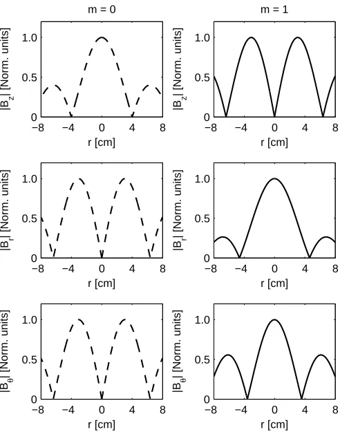
Then assuming the wave magnetic field to vary as B = B(r)ei(mθ+kzz−ωt)_{, where} _m _is

an azimuthal mode number, andr and zare radial and axial coordinates in a cylindrical coordinate system [74, 79], the general solution for theBz component is

Bz =AJm(k⊥r) +BKm(k⊥r) (1.69)

whereJm is a Bessel function of the first kind,A and B are arbitrary constants, andKm is a Bessel function of the second kind (sometimes known as a McDonald function). At

r = 0,Km(r) diverges, and thusB = 0. Therefore the general solution is [74, 79]

Bz =AJm(k⊥r) (1.70)

Similarly, and with some further algebraic simplification, the solution for the Br and Bθ components can be written as [74, 79]

Br = iA

2k⊥

[(k+kz)Jm−1(k⊥r) + (k−kz)Jm+1(k⊥r)] (1.71)

Bθ =− A

2k⊥

[(k+kz)Jm−1(k⊥r)−(k−kz)Jm+1(k⊥r)] (1.72)

If these equations are then put into Eqn. 1.5, after some algebra the electric field is found as [79]

Ez= 0 (1.73)

Er= ω