MoL 2014 22: Categorical Foundations for Extended Compositional Distributional Models of Meaning

(1)

Categorical Foundations for Extended Compositional Distributional

Models of Meaning

MSc Thesis

(Afstudeerscriptie)

written by

Gijs Wijnholds

(born May 6th, 1990 in Zwolle, The Netherlands)

under the supervision of Prof Dr Michael MoortgatandDr Raquel Fernandez, and submitted to the Board of Examiners in partial fulfillment of the requirements for the degree of

MSc in Logic

at theUniversiteit van Amsterdam.

Date of the public defense: Members of the Thesis Committee:

December 19, 2014 Dr Maria Aloni (Chair) Prof Dr Michael Moortgat Dr Raquel Fernandez Dr Nick Bezhanishvili Dr Richard Moot

(2)

Abstract

Compositional distributional models of meaning were introduced by Coecke et al. (2010, 2013) with the aim of reconciling the theory of distributional meaning in terms of vector space semantics with the theory of compositional interpretation as one finds it in typelogical grammars. The particular typelogical formalisms employed by Coecke et al. (pregroup grammars, Lambek calculus) have a recognizing capacity equivalent to context-free grammars. It is well known, however, that natural languages exhibit patterns that require expressivity beyond context-free (Huybregts, 1984; Shieber, 1987). The aim of this thesis, then, is to investigate extensions of compositional distributional models of meaning that result from using typelogical grammars with enhanced expressivity. To this end, we give a categorical characterization of the Lambek-Grishin Calculus (see Moortgat (2007, 2009) and references there) and its constituting subsystems in terms oflinear distributive categories

(3)

Acknowledgements

Firstly, I would like to express my gratitude towards my first supervisor, Michael Moortgat, for having the patience to supervise this project. Without his constant support, whether it be content wise or TEXnically, I would not have been capable of writing this thesis. Second of all, my thanks go out to my second supervisor, Raquel Fernandez, for encouraging me to take a break every now and then, and for giving helpful comments on earlier drafts of this document.

I would like to thank the remainder of my thesis committee, Maria Aloni, Nick Bezhanishvili, Mehrnoosh Sadrzadeh and Richard Moot for taking the time to read this lengthy document and to attend my thesis defense. Special thanks go out to John Baez and Peter Selinger for providing helpful comments and insights regarding string diagrams.

I also wish to thank Ulle Endriss, Michael Franke, and Raquel Fernandez for making practical arrangements to help me finish the Master of Logic after almost a year of absence. Lastly, I wish to thank Tanja Kassenaar and Gina Beekelaar from the ILLC staff for assisting me whenever necessary with any practical issues.

Furthermore, I owe special thanks to the following friends: Jim Keyni, for showing me around in Amsterdam and for the visits in Utrecht. Rob, for the endless amount of table tennis matches. Bram and Jeroen, for showing me a different side of academia. Sander, for all the fun.

I wish to thank my parents and my brother for all of the love and support they have shown throughout my life and for helping me get back on my feet again.

(4)

Introduction

The analysis of natural language can be subdivided in several parts: that of the analysis ofpatterns, which we call syntax, and the analysis of meaning association, which we call semantics. Beyond syntax and semantics proper, there is the realm of pragmatics, the analysis ofmeaning in context

rather than a conventional, static meaning. For the purpose of this study, syntax and semantics are already enough of a challenge. Form and meaning should not be considered in isolation; it is a common understanding that these two aspects of natural language are highly interdependent. Providing the link between syntax and semantics is providing the syntax-semantics interface, a method describing how the process of putting together syntactic patterns provides information as to how the meaning of these patterns should be assembled. A crucial, desirable feature of the interface between form and meaning iscompositionality, which roughly states that

The meaning of a complex expression is given by the meaning of its constituent expressions and the way in which they are combined.

The categorial approach to grammatical analysis is based on the idea that linguistic expressions are assignedtypes; thelogicfor the grammatical type system then determines what the syntactically well-formed combinations of expressions are. The syntax-semantics interface is modelled along the lines of theCurry-Howard correspondence. Orinigally developed in the context of intuitionistic logic, the CH correspondence allows one to associate logical derivations with terms of the lambda calculus, hence the slogan ‘proofs as programs’. In the application to grammars, the terms associated with a derivation serve as ‘semantic recipes’ prescribing how the meaning of a complex expression is to be computed out of the meaning of its constituent parts. A standard way of setting up semantic

models for typelogical grammars is to adopt the set-theoretic view of Montague Grammar (after (Montague, 1970b,a)): one assumes a fixed domain of entities and of truth-values on which one then defines set-theoretical constructions that give the desired meanings of complex expressions via compositionality. The problem with this approach is that the set-theoretic interpretation of the basic expressions (words) ispredefined.

(8)

complicated expressions.

A first question that arises then, is how to combine typelogical grammar with its nice mathemat-ical properties with the distributional view on lexmathemat-ical semantics. That such a combination is indeed possible is show by recent research of Coecke et al who rely on the similar mathematical structure of pregroups (a particular typelogical grammar) and finite dimensional vector spaces (Coecke et al., 2010) or on the similar mathematical structure of Lambek monoids and finite dimensional vector spaces (Coecke et al., 2013). Such similar structure implicitly relies on an extension of the Curry-Howard correspondence, initiated by Lambek and Scott in their book (Lambek and Scott, 1988), on which we will elaborate below.

Combining a substructural logic such as the Lambek Calculus with vector space semantics gives models that we will callbasic compositional distributional models of meaning. Basic, because they rely on the Lambek Calculus, the typical “logic of grammatical composition”. We shall consider deploying this very logic a weakness of the model, for the reason that the patterns that we are able to describe with this logic do not encompass all possible patterns present in natural language. It has indeed been argued that the context-free languages, the class of patterns describable by context-free grammars as well as Lambek grammars, lack the necessary expressivity (Huybregts, 1984; Shieber, 1987). We therefore raise the following problem, which will be the central theme in this study: how can we extend compositional distributional models of meaning in such a way that we can describe patterns beyond context-freeness and associate meaning to them?

Our approach in this thesis will then be to considerextensionsof the Lambek Calculus that have the proper expressivity, including at least themildly context-sensitive languages (Joshi et al., 1990). The sought extensions should exhibit a mathematical structure similar to that of finite dimensional vector spaces, making it possible to defineextended compositional distributional models of meaning. Before outlining the structure of this thesis, we give some context to place the problem in its proper setting.

Compositionality and Type-Logical Grammar

The intuitive view of compositionality that we gave at the beginning of this section assumes that (a) the meaning of the basic lexical expressions is given and that (b) the meaning of non-basic expressions can be systematically obtained from “the way in which they are combined” syntactically. This intuitive view is made more precise in (Hendriks, 2001), elaborating on (Montague, 1970b). In short, Syntax and Semantics are modelled as multisorted algebras, and compositional interpretation takes the form of ahomomorphism. i.e. a mapping from source (syntax) to target (semantics) that respects the sorts and the operations. In a picture:

Source

h(As)s∈S, Fi

Target

h(Bt)t∈T, Gi h

(9)

whereg is the semantic operation at the target end corresponding to the syntactic operationf. The benefit of compositionality is immediate: only the semantics of basic expressions is needed to obtain the semantics for larger, complex expressions. This implies that one only needs a finite specification of adictionary in order to generate an infinite amount of linguistic structures together with the corresponding interpretations.

Typelogical grammar precisely assumes compositionality as being a homomorphism from the derivational term algebra to semantics, having a logical system as the grammatical framework, on which one can easily graft a semantics that follows the structure of the complex expressions in the language. The problem then resides in lexical semantics: how does one attribute a meaning to single words? A standard tool, initiated by Montague in the ’70s (Montague, 1970b), is to employ a set-theoretic lexical semantics, in which one assumes a domain of entities and a domain of truth-values on which relations are defined. The meaning of the wordmanin this setting would be precisely the set of entities that are men, or equivalently, the characteristic function that maps all men to truth value 1 and all other entities to truth value 0; the meaning of the wordthe in combinatin with a noun is a function that picks out the unique individual that has the property denoted by the noun if there is such a unique individual, and nothing otherwise.

Non-local composition is a pervasive feature of language. Typical examples include non-periphal extraction and crossing dependencies. The former is exemplified by a expression such as “the book that John found in the library”. The relative pronoun “that” in this case has to establish a semantic dependency with the direct object of “found”, but this direct object is hidden within the relative clause, and inaccessible for external inspection. An example of crossing dependencies in Dutch is “(Ik weet) dat Jan Marie de kinderen zag leren zwemmen” (I know that John saw Mary teaching the kids how to swim). In this case the semantic dependencies can be represented by the following picture

hij denkt dat Jan Marie de kinderen wil leren zwemmen

which is a typical example of a pattern unrecognizable by context-free grammar, the copy language

w2.

(10)

related to but in key aspects different from that of Cockett and Seely (1997b). We will define linear distributive bi-clopen categories in the second part of the thesis.

A Classic: the CHL Correspondence

As said above, the Curry-Howard correspondence1 _{states an isomorphim between proofs in}

intu-itionistic propositional logic and terms of the simply typed lambda calculus. The following table gives an impression of how the different concepts of logic relate to the different concepts in lambda calculus:

Logic Lambda Calculus formula type

proof program normalization β-reduction

As was shown by Lambek and Scott (1988), this correspondence can be elevated to the level of categories, and hence it goes by the name Curry-Howard-Lambek (CHL) correspondence. It establishes an equivalence of categories2 _{between cartesian closed categories and typed lambda}

calculi with products. The great benefit of applying such a correspondence to other kinds of categories is that other kinds of logics can be seen to (categorically) be “essentially the same as” their associated category, meaning that we can also broaden our options for a syntax-semantics interface that incorporates compositionality via homomorphic passages from the type logic to the associated semantic category. The CHL correspondence is nicely shown in the following picture:

Graphical Reasoning in Logic and Categories

With the introduction of linear logic (Girard, 1987) came the introduction ofproof nets. Proof nets are graphical representations of sequent proofs that remove spurious ambiguity: going from sequent systems to natural deduction requires a many-to-one mapping that thus identifies a great deal of sequent proofs. Proof nets avoid this by implicitly representing several sequent proofs by the same net. Proof nets for the Lambek Calculus have been studied intensively (Roorda, 1991; Moot, 2002) and consequently, proof nets have been developed for the multimodal Lambek Calculus (Moot and Puite, 2002) and for the Lambek-Grishin Calculus (Moortgat and Moot, 2012).

On the side of categories, several graphical representations have been examined under the name ofstring diagrams. Here, the morphisms of the category in question can be represented graphically and one defines the appropriate equations on diagrams in order to have a coherent (i.e. sound and complete) language to reason graphically instead of chaining equations. A nice introduction to graphical reasoning in categories is (Selinger, 2011).

(12)

not just as strings but as binary trees. As a consequence, we need a whole new concept of graphical language, which we fully develop for these closed categories.

Recap: Problem Statement in Context

To summarize, the problem we have raised is as follows: because the existing compositional distri-butional models of meaning are to weak in terms of their capabilities to analyze natural language patterns, there is a need forextended compositional distributional models of meaning. Having the Curry-Howard-Lambek correspondence as our guiding light, we find that to develop such models we require the following: we should find a suitable extension of the Lambek Calculus, powerful enough to describe the mildly context-sensitive languages and exhibiting a categorical structure that isinterpretable in finite dimensional vector spaces. Next to these objectives, we want to de-velop graphical languages for the categorical structures we find, and explore a bit the semantics of the basic and the extended models.

What This Thesis is Not About

This thesis introduces a new framework for compositional distributional models of meaning. An important aspect of these models is their empirical nature; this thesis prepares the way for empirical validation of more refined compositional distributional meaning models. Actually carrying out experiments to validate the power of these models in for instance sense disambiguation and sentence similarity would be a thesis subject of its own: one might fix a grammar and then extract from a corpus the vector space semantics and see how the extended models behave with respect to the basic models. However, this still has the problem of having to predefine the lexical type declarations. Thus, it would be better to also extract the grammar (categorially: the lexicon) out of the corpus viagrammar induction. Doing grammar induction will obviously also show the difference between different syntactic backbones used. To perform multiple experiments with different set-ups would take quite some time, and we therefore leave it to future work. We will also point this out in our conclusion section.

Overview of Type-Logics

(13)

.

. . .

. . . .

. . .

.

NLr

Lr UNLr

ULr

NL

L UNL

UL NLl

Ll UNLl

ULl

where the dashed lines indicate isomorphisms between systems. The dual Grishin systems are obtained by replacing theLby aGand give rise to a similar diagram.

Finally, one obtains the Lambek-Grishin system by merging the systems NL and NG and adding interaction postulates3 _{between the two systems:}

NL NG

LG

LGIV

where the arrows indicate that each system is a part of the system it is pointing to. Of the systems NLand L(and their unital variants) it is known that they are complete with respect to (unital)

residuated groupoids and (unital)residuated semigroups respectively (see Buszkowski (1986)). For an overview of algebraic semantics for substructural logics in general, see the book by Galatos et al. (2007). We will show in this thesis that the logics under discussion all correspond to certain categorical notions to be defined in the first chapter of each part. Just as the system MLL of multiplicative linear logic with units corresponds to *-autonomous categories (Blute and Scott,

3_{The particular interaction postulates we will consider are the type IV interactions amongst a range of possible}

(14)

2004) and intuitionistic propositional logic corresponds to cartesian closed categories (Lambek and Scott, 1988), we establish correspondences according to the following tables:

NL(l/r) _{left/right/bi-closed tensor categories ((L/R/B)CC}

st)

UNL(l/r) left/right/bi-closed unitary tensor categories (U(L/R/B)CCst)

L(l/r) _{left/right/bi-closed associative tensor categories (A(L/R/B)CC}

st)

UL(l/r) _{left/right/bi-closed monoidal categories (M(L/R/B)CC}

st)

NG(l/r) _{left/right/bi-open tensor categories ((L/R/B)OC}

st)

UNG(l/r) _{left/right/bi-open unitary tensor categories (U(L/R/B)OC}

st)

G(l/r) left/right/bi-open associative tensor categories (A(L/R/B)OCst)

UG(l/r) _{left/right/bi-open monoidal categories (M(L/R/B)OC}

st)

Finally the last table shows the correspondences for the Lambek-Grishin system: LG∅ bi-clopen tensor categories (BCOCst)

LGIV linear distributive tensor categories (LDTCst)

Contributions and Structure of the Thesis

In this thesis, we develop a uniform framework for doing compositional distributional semantics guided by the work of Coecke et al. (Coecke et al., 2010, 2013). More specifically, in part I we review and expand where necessary the theory of basic categorical compositional distributional models of meaning by the following chapters:

Chapter 1We introduce basic category theory and categories with additional structure. Chapter 2We introduce graphical languages for categories with additional structure. The first contribution is the development of a coherent graphical language for non-associative systems. Chapter 3We introduce Lambek’s Syntactic Calculus and present its “categorification”. Chapter 4We review finite-dimensional vector spaces as a system of doing distributional semantics and show how a compositional distributional model of meaning could be obtained.

(15)

Chapter 5We introduce co-closed (or open) categories and non-associative linearly

(16)

Part I

(17)

Chapter 1

Categories

(18)

A category essentially is an abstraction over mathematical structures: it contains objects and arrows between objects, the latter of which can be composed to construct new arrows. Additionally some evident axioms need to be satisfied: there must be identity arrows for every object and composition of arrows should beassociative. From this concept of category, one can go on to define

arrows between categories, these are called functors. Then one will want to define arrows between functors, to be called natural transformations. The nice thing about the theory of categories is that we can view functors as arrows between categories, but also as the arrows of a category that has categories as objects, or we may even think of them as objects of a category, the arrows now being the natural transformations. These shifts in viewpoint are characteristic (and may lead to confusion) for category theory. Some additional concepts include that of adjunction, which will be a key concept in the rest of this thesis, and the concept ofmonads, which we use to illustrate the categorical structure of the type logics we will consider. We will start out with the very basic concepts and work our way through categories with extra structure.

1.1 The Basics

The most basic definition in category theory consists of that of category: Definition 1.1. A category Cconsists of:

• A collection of objectsOb(C), denoted byA, B etc.,

• A collection of morphismsAr(C), denoted byf, g etc.,

• Mappingsdom, cod:Ar(C)→Ob(C) assigning to each morphism its domain and codomain respectively. We writef :A→B for a morphismf withdom(f) =Aandcod(f) =B.

• Identity arrows, i.e. for every objectAthere is an arrowidA:A→A,

• Composition of arrows, i.e. for every morphisms f : A → B and g : B → C there is a composite morphismg◦f :A→C.

These data must satisfy the following equations:

h◦(g◦f) = (h◦g)◦f forf :A→B,g:B→C,h:C→D,

f◦idA=f =idB◦f forf :A→B.

We define, for a category C and two objects A, B in Ob(C), the Hom-set of A and B as

HomC₍_{A, B}_{) :=}_{_f _∈_Ar_(C)_|_f _:_A_→_B_}_.

For anyf :A→BinC, we say thatf is an isomorphism when there exists a two-sided inverse, i.e. ag:B→A such thatg◦f =idA andf◦g=idB.

We will introduce the notion ofopposite or dual category as a preliminary for duality:

Definition 1.2(Dual Category). Given a categoryC, its dual categoryCop is given by considering the following construction:

• The objectsOb(Cop) are precisely Ob(C),

• The morphisms Ar(Cop) are precisely Ar(C),

(19)

• Composition is reversed, i.e. g◦f becomesf◦g.

A lot of examples of categories involve certain mathematical structures and homomorphisms between these structures. One could also think of a category as a structure, and define the structure homomorphisms categorically. These are called functors:

Definition 1.3. A (covariant) functor F : C → D is a mapping that assigns to each object A

in Ob(C) an object F(A) in Ob(D) and to each morphism f : A → B in Ar(C) a morphism

F(f) :F(A)→F(B) inAr(D) such that the following hold: 1. F(g◦f) =F(g)◦F(f),

2. F(idA) =idF(A).

Besides a regular functor (the lifting of an direction preserving homomorphism), there are also direction reversing homomorphisms in category theory, called contravariant functors:

Definition 1.4. A contravariant functor F : C → D is a mapping that assigns to each object

A in Ob(C) an object F(A) in Ob(D) and to each morphism f : A → B in Ar(C) a morphism

F(f) :F(B)→F(A) inAr(D) such that the following hold: 1. F(g◦f) =F(f)◦F(g),

2. F(idA) =idF(A).

Since we have introduced the notion of dual category, we note here that a contravariant functor

F :C→D is the same as a covariant functorF :Cop→D.

Similarly to the case of morphisms, there are identity functors and there exists associative composition of functors. So, it makes sense to define isomorphisms of categories: we say that

F : C → D is an isomorphism of categories if there exists a functor G : D → C such that

G◦F=IdCandF◦G=IdD.

Finally, we wish to reserve a special place forbifunctors, functors that take two arguments. We denote such a functor byF :C×D→Ewhere C×Dis the product category, the category that has pairs of objects as objects and pairs of morphisms as morphisms. As a consequence, we express the functorial restrictions (or bifunctoriality) as the following two restrictions:

• Identities should be preserved, soF(id(A,B)) =idF(A,B),

• Composition should be preserved, soF((k, h)◦(g, f)) =F(k, h)◦F(g, f). Next are the “arrows between functors”, ornatural transformations:

Definition 1.5. For two functorsF, G:C→D, a natural transformation θ:F →Gis a family of morphisms θA : F(A) → G(A) (one for every A in Ob(C)) such that for any f : A → B the

equationθB◦F(f) =G(f)◦θAholds, i.e. the following diagram commutes: F(A) G(A)

F(B) G(B)

θA

F(f) G(f)

(20)

For functorsF, G:C→D, a natural transformationθ:F →Gis a natural isomorphism if for everyAinOb(C) we have thatθA:F(A)→G(A) is an isomorphism. We writeF∼=Gto say that

F is naturally isomorphic to G.

Because many categories are not necessarily isomorphic, but rather isomorphic up to natural isomorphism, we need to define the concept of anequivalence of categories:

An equivalence of categories consists of a functor F :C →D and a functorG:D→ C such thatG◦F ∼=IdC andF◦G∼=IdD. We denote the equivalence of categories byC∼=D.

We now turn to the most important categorical concept for our purposes and perhaps the most important concept in basic category theory: the concept ofadjunction. Adjunction coversGalois connections in order theory, but it also captures the behaviour of the universal quantifier versus that of the existential quantifier in first-order logic (Awodey, 2006, Section 9.5). We will proceed to give three equivalent definitions of adjunction, however we will mostly use theHom-set definition: Definition 1.6(Hom-set Adjunction). Given two categoriesCandD, an adjunction between two functors F : C → D and G : D → C consists of a natural isomorphism ϕ : HomD(F A, B) ∼=

HomC(A, GB).

The other definitions are given in terms of the unit orco-unit of the adjunction together with a universal mapping property:

Definition 1.7 (Unit Adjunction). Given two categories C and D, an adjunction between two functorsF :C →D and G:D→ C consists of a natural transformation η :IdC→ G◦F such that for any objectA in C andB in D and any morphismf :A →G(B), there exists a unique

g:F(A)→B such thatf =G(g)◦ηA.

Definition 1.8(Co-Unit Adjunction). Given two categoriesCandD, an adjunction between two functorsF : C→ Dand G: D→C consists of a natural transformation :F ◦G→IdD such that for any objectA in C and B in D and any morphism g : F(A)→ B there exists a unique

f :A→G(B) such thatg=B◦F(f).

See (Awodey, 2006, Chapter 9) for a proof that these definitions are in fact equivalent.

The concept of a monad, also called a triple or standard construction, might be seen as the generalization of the concept of aclosure operator in order theory:

Definition 1.9. A monad on a categoryCis a triple (T, η, µ) whereT :C→Cis an endofunctor andη:IdC →T andµ:T ◦T →T are natural transformations such that the following diagrams

commute for every objectA:

T(T(T(A))) T(T(A))

T(T(A)) T(A)

T(µA)

µT(A) µA

µA

T(A) T(T(A))

T(A)

T(ηA)

idT(A) µA

T(A) T(T(A))

T(A)

ηT(A)

(21)

The striking thing about mondads is that two adjoint functors always define a monad! Note that in the following proposition we use the notationGF: this is the natural transformation defined forAinOb(C) asG(F(A)).

Proposition 1.1. Given two functors F : C → D and G : D → C that are adjoint, the triple

(G◦F, η, GF) where η is the unit of the adjunction and is the co-unit of the adjunction is a monad.

Next to considering closure operators and monads as their generalization, we want to note that the dual notion, that of aninterior operator, is generalized by the dual notion of acomonad: Definition 1.10. A comonad on a category C is a triple (S, ϑ, υ) whereT : C→C is an endo-functor andϑ:S →IdC and υ :T →T ◦T are natural transformations such that the following diagrams commute for every objectB:

S(S(S(B))) S(S(B))

S(S(B)) _υ S(B)

B

υB ϑS(B)

S(ϑB)

S(B) S(S(B))

S(B)

S(ϑB)

idS(B) υB

S(B) S(S(B))

S(B)

ϑS(B)

idS(B) υB

We then get that the reversed compositionF ◦Gfor adjoint functors F and Ggives rise to a comonad:

Proposition 1.2. Given two functors F : C → D and G : D → C that are adjoint, the triple

(F◦G, , F ηG), where η is the unit of the adjunction and is the co-unit of the adjunction, is a comonad.

In the next section, we will look atcategories with additional structure.

1.2 Monoidal and Closed Categories

A standard concept of a category with extra structure is that of amonoidal category: a category that exhibits the structure of a monoid. However, for our purposes we need to simplify this definition as we want to consider categories with extra structure but without associativity or units. To this end we definetensor categories1_{as categories that have a “tensor” without extra coherence axioms}

whatsoever:

Definition 1.11. A tensor category is a categoryCequipped with a bifunctor⊗:C×C→C.

1_{The term tensor category seems to be used to refer to a monoidal category. Despite the confusion, we found it}

(22)

We can then go on toadd associativity or units, giving us the following definitions:

Definition 1.12. An associative tensor category (or non-unitary monoidal category) is a tensor category (C,⊗) equipped with an isomorphism natural in A, B, C specified byαA,B,C : (A⊗B)⊗

C→A⊗(B⊗C) where the following diagram commutes:

(A⊗(B⊗C))⊗D A⊗((B⊗C)⊗D)

((A⊗B)⊗C)⊗D A⊗(B⊗(C⊗D))

(A⊗B)⊗(C⊗D)

αA,B⊗C,D

idA⊗αB,C,D

αA,B,C⊗idD

αA⊗B,C,D αA,B,C⊗D

Definition 1.13. A unitary tensor category (or non-associative monoidal category) is a tensor category (C,⊗) with a distinguished unit object I and natural isomorphisms specified by λA : I⊗A→AandρA:A⊗I→A.

Definition 1.14. A monoidal category (or associative unitary tensor category) is an associative unitary tensor category (C,⊗, α, I, λ, ρ) where the following diagram commutes:

(A⊗I)⊗B A⊗(I⊗B)

A⊗B

αA,I,B

ρA⊗idB idA⊗λB

We have now sketched one dimension in our landscape of categories: adding a tensor and then picking a unit object or associativity as extra features to ultimately obtain a monoidal category. There are also monoidal categories where the tensor behaves as a commutative product:

Definition 1.15. A symmetric monoidal category is a monoidal category (C,⊗, α, I, λ, ρ) equipped with natural isomorphisms specified bycA,B:A⊗B →B⊗Asuch thatcB,A◦cA,B=idA⊗B and

such that the following diagrams commute:

(B⊗A)⊗C B⊗(A⊗C)

(A⊗B)⊗C B⊗(C⊗A)

A⊗(B⊗C) (B⊗C)⊗A

αB,A,C

idB⊗cA,C cA,B⊗idC

αA,B,C

cA,B⊗C

(23)

A⊗I I⊗A

A cA,I

ρA λA

We now want to define theclosure of our categories. This is achieved by adding bifunctors that are left/right adjoint to the tensor:

Definition 1.16. A left closed tensor category is a tensor category (C,⊗) equipped with a bifunctor

⇒:Cop×C→C(i.e. contravariant in its first argument, covariant in its second argument) together with natural isomorphism specified byβA,B,C :HomC₍_A_⊗_{B, C}₎_→_HomC₍_{B, A}_⇒_C_).

Definition 1.17. A right closed tensor category is tensor category (C,⊗) equipped with a bifunctor

⇐:C×Cop→C together with a natural isomorphism specified byγA,B,C :HomC(A⊗B, C)→

HomC(A, C⇐B).

Definition 1.18. A bi-closed tensor category is a tensor category (C,⊗) that is both left and right closed.

Left closed, right closed, and bi-closed associative tensor/monoidal categories are defined anal-ogously. Note, however, that a symmetric monoidal category is by definition bi-closed when it is either left or right closed. For example, suppose we have a left closed symmetric monoidal category (C,⊗, α, I, λ, ρ, c,⇒, β). DefineB ⇐A:=A⇒B andγ :=f 7→β(f◦c). It is easy to show that this defines a right closed structure onC.

We have already noted that adjoints give rise to monads and comonads. However, there are another two monads that arise in bi-closed categories:

Let (C,⊗,⇒, β,⇐, γ) be a bi-closed category. Define, for any objectD in Ob(C) the functor

D⇐( ⇒D) (resp. (D⇐ )⇒D ) that sends objects AtoD⇐(A⇒D) ( (D⇐A)⇒D) and sends mapsf :A→B toidD⇐(f ⇒idD) ( (idD⇐f)⇒idD ).

Now define the natural transformationsη:IdC→D⇐( ⇒D) byηA:=γ(β−1(idA⇒D)) and µ: D ⇐((D ⇐( ⇒D))⇒D) by µA := idD ⇐(β(γ−1(idD⇐(idA⇒D)))) (and similarly for the

functor (D⇐ )⇒D.

Proposition 1.3. The triple(D⇐( ⇒D), η, µ)defines a monad onC. Proof. For the square diagram we have

(idD⇐(β(γ−1(idD⇐(A⇒D)))))◦(idD⇐((idD⇐(β(γ−1(idD⇐(A⇒D)))))⇒idD))

=idD⇐((idD⇐(β(γ−1(idD⇐(A⇒D)))))⇒idD◦β(γ−1(idD⇐(A⇒D))))

=idD⇐((idD⇐(β(γ−1(idD⇐(A⇒D)))))⇒idD◦β(γ−1(idD⇐(A⇒D)))◦idA⇒D)

=idD⇐(β(idD◦γ−1(idD⇐(A⇒D))◦((idD⇐(β(γ−1(idD⇐(A⇒D))))⊕idA⇒D)))

=idD⇐(β(γ−1((idD⇐(idA⇒D))◦idD⇐(A⇒D)◦(idD⇐(β(γ−1(idD⇐(A⇒D))))))))

=idD⇐(β(γ−1(idD⇐(A⇒D)◦idD⇐(A⇒D)◦(idD⇐(β(γ−1(idD⇐(A⇒D))))))))

=idD⇐(β(γ−1((idD⇐(β(γ−1(idD⇐(A⇒D)))))◦idD⇐((D⇐(A⇒D))⇒D)◦idD⇐((D⇐(A⇒D))⇒D))))

=idD⇐(β(idD◦γ−1(idD⇐((D⇐(A⇒D))⇒D))◦(idD⇐((D⇐(A⇒D))⇒D)⊗β(γ−1(idD⇐(A⇒D))))))

=idD⇐((idD⇐((D⇐(A⇒D))⇒D)⇒idD)◦β(γ−1(idD⇐((D⇐(A⇒D))⇒D)))◦β(γ−1(idD⇐(A⇒D))))

=idD⇐(id(D⇐((D⇐(A⇒D))⇒D))⇒D◦β(γ−1(idD⇐((D⇐(A⇒D))⇒D)))◦β(γ−1(idD⇐(A⇒D))))

=idD⇐(β(γ−1₍_id

D⇐((D⇐(A⇒D))⇒D)))◦β(γ−1(idD⇐(A⇒D))))

= (idD⇐(β(γ−1₍_id

(24)

For the first triangle diagram, we have (idD⇐(β(γ−1₍_id

D⇐(A⇒D)))))◦(idD⇐((γ(β−1(idA⇒D)))⇒idD))

=idD⇐(((γ(β−1₍_idA

⇒D)))⇒idD)◦β(γ−1(idD⇐(A⇒D)))) bifunctoriality of⇐

=idD⇐(((γ(β−1₍_idA

⇒D)))⇒idD)◦β(γ−1(idD⇐(A⇒D)))◦idA⇒D) identity axiom

=idD⇐(β(idD◦γ−1₍_id

D⇐(A⇒D))◦(γ(β−1(idA⇒D))⊕idA⇒D))) naturality ofβ

=idD⇐(β(γ−1((idD⇐idA⇒D)◦idD⇐(A⇒D)◦γ(β−1(idA⇒D))))) naturality ofγ−1

=idD⇐(β(γ−1(idD⇐(A⇒D)◦idD⇐(A⇒D)◦γ(β−1(idA⇒D))))) bifunctoriality of⇐

=idD⇐(β(γ−1(γ(β−1idA⇒D)))) identity axiom twice

=idD⇐idA⇒D iso property ofβ andγ

=idD⇐(A⇒D) bifunctoriality of⇐

Finally, for the second triangle diagram, we have

(idD⇐(β(γ−1(idD⇐(A⇒D)))))◦γ(β−1(id(D⇐(A⇒D))⇒D))

= (idD⇐(β(γ−1(idD⇐(A⇒D)))))◦γ(β−1(id(D⇐(A⇒D))⇒D))◦idD⇐(A⇒D) identity axiom

=γ(idD◦β−1(id(D⇐(A⇒D))⇒D))◦(idD⇐(A⇒D)⊗β(γ−1(idD⇐(A⇒D)))) naturality ofγ

=γ(β−1₍₍_id

D⇐(A⇒D)⇒idD)◦id(D⇐(A⇒D))⇒D◦β(γ−1(idD⇐(A⇒D))))) naturality ofβ−1

=γ(β−1₍_id

(D⇐(A⇒D))⇒D◦id(D⇐(A⇒D))⇒D◦β(γ−1(idD⇐(A⇒D))))) bifunctoriality of⇒

=γ(β−1₍_β₍_γ−1_id

D⇐(A⇒D)))) identity axiom twice

=idD⇐(A⇒D) iso property ofβ andγ

Next to the closed categories we have already considered, there are special cases of a monoidal closed category, where each object has a left/right dual object. When the underlying category is non-symmetric, such a category is called autonomous or rigid but in the presence of symmetry these categories are calledcompact closed:

Definition 1.19. An autonomous category is a monoidal category (C,⊗, α, I, λ, ρ) such that for every objectAinOb(C) there exist objectsAlandAr(called left and right adjoints) and for every A there exist morphisms

ηl_:_I_→_A_⊗_Al l_:_Al_⊗_A_→_I _ηr_:_I_→_Ar_⊗_A r_:_A_⊗_Ar_→_I

(25)

(A⊗Al₎_⊗_A _A_⊗₍_Al_⊗_A₎

I⊗A A⊗I

A A

α_{A,Al ,A}

idA⊗l ηl⊗idA

ρA λ−_A1

idA

Al⊗(A⊗Al) (Al⊗A)⊗Al

Al⊗I I⊗Al

Al Al

α−1 Al ,A,Al

l⊗id_Al id_Al⊗ηl

λA ρ−1

Al

id_Al

A⊗(Ar⊗A) (A⊗Ar)⊗A

A⊗I I⊗A

A A

α−_{A,Ar ,A}1

r⊗idA idA⊗ηr

λA ρ−_A1

idA

(Ar_⊗_A₎_⊗_Ar _Ar_⊗₍_A_⊗_Ar₎

I⊗Ar _Ar_⊗_I

Ar _Ar

αAr ,A,Ar

idAr⊗r ηr_⊗_id

Ar

ρAr λ−1

Ar

idAr

Autonomous categories as defined above should actually be called bi-autonomous categories as they contain both left and right dual objects. It is of course obvious how left/right autonomous categories should be defined. In the case that the monoidal category is also symmetric, the left and right dual objects collapse into one dual object (up to isomorphism) and we speak of a compact closed category.

An interesting property of autonomous and compact closed categories is that they form bi-closed categories by settingA ⇒B :=Al⊗B and B ⇐A :=B⊗Ar, giving rise to the following two propositions:

Proposition 1.4. Every bi-autonomous category is a bi-closed tensor category.

Proposition 1.5. Every compact closed category is a bi-closed symmetric monoidal category.

In the following section, we consider functors with structure for use between the various kinds of categories we have considered so far.

1.3 Monoidal and Closed Functors

Definition 1.20. For (C,⊗) and (D,•) tensor categories, a tensor functor is a functorF :C→D such that there exists a natural transformation specified byϕA,B:F A•F B→F(A⊗B).

(26)

(F A•F B)•F C F A•(F B•F C)

F(A⊗B)•F C F A•F(B⊗C)

F((A⊗B)⊗C) F(A⊗(B⊗C))

α0_{F A,F B,F C}

ϕA,B•idF C idF A•ϕB,C

ϕA⊗B,C ϕA,B⊗C

F αA,B,C

Definition 1.22. For (C,⊗, α, I, λ, ρ) and (D,•, α0,1, λ0, ρ0) monoidal categories, a monoidal func-tor is an associative tensor funcfunc-torF :C→Dwith associated natural transformation specified by

ϕA,B :F A•F B→F(A⊗B) and there exists a morphismψ: 1→F I such that additionally the

following diagrams commute:

F A•F I F(A⊗I)

F A•1 F A

ϕA,I

F ρA idF A•ψ

ρ0_{F A}

F I•F B F(I⊗B)

1•F B F B ϕI,B

F λB ψ•idF B

λ0_{F B}

Definition 1.23. For (C,⊗,⇒, β) and (D,•,₍, β0) left closed tensor categories, a left closed tensor functor is a tensor functor F with associated natural transformation specified by ϕA,B :

F A•F B → F(A⊗B) such that there additionally exists a natural transformation specified by

χA,B:F(A⇒B)→F A₍F Bsuch that for everyf :A⊗B→CinC, we have that the following diagram commutes:

F B F(A⇒C)

F A₍F C

F(β(f))

β0(F(f)◦ϕA,B) χA,C

Definition 1.24. For (C,⊗,⇐, γ) and (D,•, ₍ , γ0) right closed tensor categories, a right closed tensor functor is a tensor functor F with associated natural transformation specified by ϕA,B :

F A•F B → F(A⊗B) such that there additionally exists a natural transformation specified by

ξA,B:F(B⇐A)→F B ₍ F Asuch that for everyf :A⊗B→C inC, we have that the following diagram commutes:

F A F(C⇐B)

F C ₍ F B F(γ0_(f))

(27)

Definition 1.25. For (C,⊗,⇒,⇐, β, γ) and (D,•,₍, ₍ , β0, γ0) closed tensor categories, a bi-closed tensor functor is a left and right bi-closed tensor functorF.

In the final section of this chapter, we review the symmetry exhibited between left and right closed categories.

1.4 Symmetry

There is an obvious symmetry between a left and right closed category, whether it be a tensor category or a monoidal one. The symmetry involves swapping the ⇒ and ⇐ functors. So, let (C,⊗,⇒, β) be a left closed tensor category and let (D,⊗,⇐, γ) be a right closed tensor category such thatCandDhave the same objects. Define the following functorS:C→D:

S(A) = A

S(A⊗B) = S(B)⊗S(A)

S(A⇒B) = S(B)⇐S(A)

S(idA) = idS(A) S(g◦f) = S(g)◦S(f)

S(f⊗g) = S(g)⊗S(f)

S(f ⇒g) = S(g)⇐S(f)

S(β(f)) = γ(S(f))

To show that this is in fact an isomorphism of categories, define the following functorS0:D→C:

S0(A) = A

S0(A⊗B) = S0(B)⊗S0(A)

S0(B⇐A) = S0(A)⇒S0(B)

S0(idA) = idS0_(A)

S0(g◦f) = S0(g)◦S0(f)

S0(f⊗g) = S0(g)⊗S0(f)

S0(g⇐f) = S0(f)⇒S0(g)

S0(γ(f)) = β(S0(f))

It is an easy exercise to check thatS◦S0 =IdD andS0◦S =IdC.

(28)

Chapter 2

Graphical Languages

(29)

2.1 Graphical Languages: an Introduction

Reasoning about morphism equality in categories usually proceeds by drawing commutative dia-grams or explicitly writing down chains of equations. The problem with the latter form is imme-diate: it is very tedious to write down and to check whether each step is correct. One problem with commutative diagrams is that they only reflect the typing of morphisms, i.e. their domain and codomain. Nothing is said about the structure of the morphisms. So, we may very well ask ourselveshow can we represent (the structure of ) morphisms and their equations graphically?

The short answer is: just define a graphical language for the category you like! The sad news is that one will want to showcoherence, i.e. soundness and completeness of the graphical language with respect to the category it is stated for. This is usually quite hard, as it requires a considerable amount of topology.

Nevertheless, graphical languages have already been developed for monoidal categories (Joyal and Street, 1991a) and various kinds of monoidal categories with additional structure (Joyal and Street, 1991b), together with coherence proofs. For monoidal closed categories, there is a graphical language (Baez and Stay, 2011), but coherence has not been proven for it (John Baez, personal communication). A nice survey of the various graphical languages is due to Selinger (Selinger, 2011).

We will review the existing graphical languages for monoidal categories and their extension to monoidal closed categories. Then will ask ourselves what happens when we drop associativity and the units and get to the point where we want a graphical language for closed tensor categories. We provide an answer in terms ofproof netsand show coherence for a graphical language of proof nets for bi-closed tensor categories.

2.2 Graphical Languages for Monoidal Categories

We start out by representing objects in a category as labelled wires and morphisms asboxes(with their name on it) that have an incoming and an outgoing wire (resp. the domain and codomain). The identity morphism is then visualized as an ongoing wire without a box in between. Composition is defined as juxtaposing two diagrams. All this is summarized in the following figure:

Object Morphism Identity Composition

A f :A→B idA:A→A g◦f

A f

A

B

A

f

g A

B

C

(30)

2.2.1 Going Monoidal

The next step is to consider the tensor product of monoidal categories: we can draw objectsA⊗B

simply by drawing them next to each other. The unit object is represent by the empty wire, and the tensor product of morphisms is represented by drawing the morphisms next to each other. This is all in the next figure:

Tensor Product Unit object Morphism Tensor Product

A⊗B I f :A1⊗...⊗An→B1⊗...⊗Bm f⊗g

A B

...

f

...

A1 An

B1 Bm

f g

A

C B

D

Associativity of the tensor is now automatically satisfied. Also, the unit laws are immediately satisfied as we don’t bother to draw the units. In fact, we get the following coherence theorem for this graphical language:

Theorem 2.1 ((Selinger, 2011),Thm. 1.3,(Joyal and Street, 1991a), Thm. 1.2). A well-formed equation between morphisms in a monoidal category follows from the axioms if and only if it holds, up to planar isotopy, in the corresponding graphical language.

For a detailed exposition of the proof, see Joyal and Street’s original paper (Joyal and Street, 1991a). For a somewhat clearer but less detailed exposition, see the survey paper of Selinger (2011).

2.2.2 Closing the Category

We will now consider the graphical language for monoidal closed categories proposed by Baez and Stay (2011). To realize the extension of graphical languages for monoidal categories to those that have internal homs, one needs a graphical representation of objectsA⇒BandB⇐A. Intuitively, one might want to draw the objectA⇒B as an arrow going up next to an arrow going down, as in

=

A⇒B A B

However, as Baez and Stay note, in the general case where the monoidal closed category is not compact, arrows pointing up are not allowed. To resolve this issue but still maintain the intuitive idea of an arrow going upwards, one draws aclasp connecting the upwards pointed arrow to the downward pointed arrow. So for bi-closed monoidal categories, we extend the graphical language for monoidal categories with the constructs of Figure 2.1.

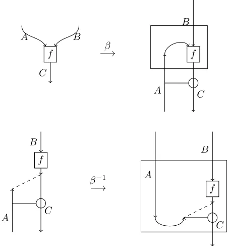
Now we only need to describe the effect ofβ andγ on morphisms graphically. The effect ofβ

andβ−1_{is shown in Figure 2.2, the graphical representation of the action of}_γ_and_γ−1_{is completely}

(31)

A⇒B B ⇐A

[image:31.612.246.371.94.174.2]

A B B A

Figure 2.1: Language Constructs for Closedness in Monoidal Categories

f −→β f

A B

C

B

A _C

f

−→

β−1

f B

C A

A

B

C

Figure 2.2: Currying and Uncurrying in Monoidal Closed Categories

Note that we have actually bent around arrows in order to keep morphisms going down. As in the general (the non-compact) case this is not allowed, we draw a box around the “illegal” constructs.

2.2.3 A Problem With the Clasp Language

Unfortunately, there is no coherence proof for the clasp language of Baez and Stay. At least the original authors have not tried to prove coherence for it (John Baez, pers. comm.). So in this subsection we will discuss some issues regarding the clasp language.

[image:31.612.193.421.222.465.2]

(32)

Given morphismsf :C→Aandg:B →D represented by

f C

A

g B

D

it makes sense to definef ⇒g as follows:

f g

B

D C

C

A A

Adopting this graphical representation, consider the fact thatidA ⇒ idB =idA⇒B should be

satisfied. This would mean that we should be able to derive

B

D C

C

A A

= A B

But the only way to do this is to require the graphical yanking equations

= =

Now consider the fact that β and γ should be natural isomorphisms: this means that the effect of consecutively currying and uncurrying some morphism should return something that is derivationally equal to the original morphims. But the currying and uncurrying of a morphism

(33)

f −→β f β−→

−1

f

A B

C

B

A _C

A

B

C

And again, the only way to make β an isomorphism is to require graphical yanking, in which case we would get

f

= f

A

B

C

A B

C

Fortunately, one can actually allow yanking when one allows it only inside a box. This means effectively that inside a box the situation is compact, while outside a box it is purely monoidal. It should however be noted that when boxes are drawn every time there is an arrow bent around, allowing yanking only within a box basically amounts to global yanking. So it might be interesting to see a definitive proof of why this does not pose a problem.

Finally, there is a problem with the concept of clasps. Consider the co-evaluation morphism

(34)

B

A⊗B A

Clearly, there are some problems with the clasp language as we have considered it. Either cer-tain constructs should be made explicit to be able to have a coherent graphical language based on clasps, or it should not be attempted to recover a coherent language from the clasp diagrams.

In the next section we will develop a graphical language for closed tensor categories and prove coherence for it.

2.3 Graphical Languages for Closed Tensor Categories

In this section, we develop a graphical language for closed tensor categories. That is, categories that do have a tensor and left and right internal homs but for which the tensor lacks associativity. We will see in the next chapter that these categories correspond to non-associative Lambek Calculi. We will start out with a brief review of proof nets for the latter calculi and then go on to define

proof net categoriesand state a freeness theorem about them, providing coherence for our graphical language.

2.3.1 Proof Nets versus Graphical Languages

(35)

The key difference between proof nets and graphical languages is that the former are based on sequent systems, and as such facilitate multiple “inputs” whereas morphisms in a category only have one input (i.e. the domain). So even though we take inspiration from proof nets in the development of our graphical language (we will define links, proof structures and correctness criteria) the graphical language is still very different from the proof net representation. Another difference is that proof nets can be used to give a graphical proof of cut elimination, as is done by Moot (2002, Section 4.4) for the case of multiplicative linear logic.

We will develop our proof net language taking inspiration from the work of Blute et al. (1996); Cockett and Seely (1997a) and we will prove coherence according to the method outlined in Selinger (2011).

2.3.2 Signatures, Interpretations and Free Categories

Definition 2.1. A bi-closed tensor signature Σ = (Σ0,Σ1, dom, cod) consists of:

• a set Σ0of object variables,

• a set Σ1of morphism variables,

• two mapsdom, cod: Σ1→CT(Σ0).

whereCT(Σ0) is the free (⊗,⇒,⇐)-algebra generated by Σ0.

Definition 2.2. Given a bi-closed tensor signature Σ and a closed tensor categoryC, an interpre-tationi: Σ→C consists of:

• an object mapi0: Σ0→Ob(C) such that

i0(A⊗B) =i0(A)⊗i0(B)

i0(A⇒B) =i0(A)⇒i0(B)

i0(B⇐A) =i0(B)⇐i0(A),

• for everyf ∈Σ1 a morphismi1(f) :i0(dom(f))→i0(cod(f)).

Definition 2.3. A bi-closed tensor categoryCis a free bi-closed tensor category over a bi-closed tensor signature Σ if there is an interpretation i : Σ → C such that for any bi-closed tensor categoryDand bi-closed tensor interpretationj: Σ→D, there is a unique bi-closed tensor functor

F :C→D such thatj=F◦i.

We will develop a graphical language as a proof net category. Showing that for any bi-closed tensor category, the associated proof net category is the free one means that all equations in the category hold if and only if they hold in the graphical language and as such, coherence will have been proven.

2.3.3 Sequent Calculus Categorified

(36)

Definition 2.4 (Formulae). Given a set of atomic formulaeAt, the set of formulae is defined as follows:

A, B:=p|A⊗B |A\B | B/Aforp∈At.

Next to defining formulae are structures, which will be used on the left-hand side of the turnstile in sequent proofs:

Definition 2.5 (Structures). Structures are defined over formulas using a binary merger: Γ,∆ :=A|(Γ•∆)

To ease our reading of the sequent calculus rules, we define contexts, which are structures with a unique hole in them, where we in turn can place structures in:

Definition 2.6 (Contexts). A context is a structure with a unique occurrence of a hole []: Γ[],∆[] := []|(Γ[]•∆) |(Γ•∆[])

We write Γ[∆] for replacing the hole [] in Γ by ∆.

We are now ready to define the rules of the sequent calculus for the system NL:

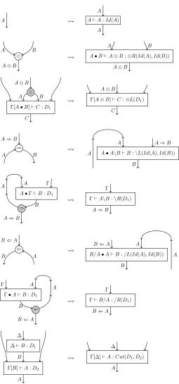
Definition 2.7 (Sequent Calculus). The sequent calculus presentation ofNLis as follows:

A`A Id

∆`B Γ[B]`A

Γ[∆]`A Cut

Γ[A•B]`C

Γ[A⊗B]`C ⊗L

Γ`A ∆`B

Γ•∆`A⊗B ⊗R

∆`B Γ[A]`C

Γ[∆•B\A]`C \L

B•Γ`A

Γ`B\A \R

∆`B Γ[A]`C

Γ[A/B•∆]`C /L

Γ•B`A

Γ`A/B /R

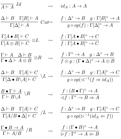
In order to “categorify” the sequent calculus, we define an equivalence relation on proofs. For this purpose, note that we can write down proofs as bracketed strings instead of drawing a whole proof tree. This is done by writing down the rule’s name and, in brackets the proofs that the rule acts upon, in the order they are listed in sequent rule. For instance, ⊗L(⊗R(Id(A), Id(B))) is a proof ofA⊗B`A⊗B. We denote byDi (fori∈N) arbitrary proofs where we use the notation

LHS(Di) = Γ andRHS(Di) =Ato denote the components of the sequent thatDi is a proof of. Our equivalence relation followsidentity unfolding andcut-elimination:

Definition 2.8. We define the following equivalence relation on sequent proofs:

• Identity unfolding, by which we mean

⊗L(⊗R(Id(A), Id(B)))≡Id(A⊗B)

\R(\L(Id(A), Id(B)))≡Id(A\B)

(37)

• Cut-elimination base case, by which we mean

Cut(D1, Id(A))≡D1 Cut(Id(B), D1)≡D1

• Principal cut-elimination, by which we mean

Cut(⊗R(D1, D2),⊗L(D3))≡Cut(D2, Cut(D1, D3))

Cut(⊗R(D1, D2),⊗L(D3))≡Cut(D1, Cut(D2, D3))

Cut(\R(D1),\L(D2, D3))≡Cut(Cut(D2, D1), D3)

Cut(\R(D1),\L(D2, D3))≡Cut(D2, Cut(D1, D3)) Cut(/R(D1), /L(D2, D3))≡Cut(Cut(D2, D1), D3) Cut(/R(D1), /L(D2, D3))≡Cut(D2, Cut(D1, D3))

• Permutative cut-elimination, by which we mean

Cut(⊗L(D1), D2)≡ ⊗L(Cut(D1, D2))

Cut(\L(D1, D2), D3)≡ \L(D1, Cut(D2, D3))

Cut(/L(D1, D2), D3)≡/L(D1, Cut(D2, D3))

Cut(D1,⊗L(D2))≡ ⊗L(Cut(D1, D2))

Cut(D1,\R(D2))≡ \R(Cut(D1, D2))

Cut(D1, /R(D2))≡/R(Cut(D1, D2)) Cut(D1,⊗R(D2, D3))≡ ⊗R(D2, Cut(D1, D3))

whenRHS(D1) =C andLHS(D3) = Γ0[C] Cut(D1,⊗R(D2, D3))≡ ⊗R(Cut(D1, D2), D3)

whenRHS(D1) =C andLHS(D2) = Γ[C]

Cut(D1,\L(D2, D3))≡ \L(D2, Cut(D1, D3)) whenRHS(D1) =C andLHS(D3) = Γ[C][A]

Cut(D1,\L(D2, D3))≡ \L(Cut(D1, D2), D3) whenRHS(D1) =C andLHS(D2) = Γ0[C]

Cut(D1, /L(D2, D3))≡/L(D2, Cut(D1, D3))

whenRHS(D1) =C andLHS(D3) = Γ[C][A] Cut(D1, /L(D2, D3))≡/L(Cut(D1, D2), D3)

(38)

2.3.4 Proof Nets Defined

We will now defineproof netsthat we will prove to correspond to bi-closed tensor categories in the sense that well-formed equations between morphisms in a bi-closed tensor category hold if and only if they hold in their graphical language. The idea is that we can build up arbitrary proof structures (possible proof nets) by gluing togetherlinks and that some correctness criteria define a subclass ofproof nets. We define some critical equations on proof structures that will give us the right tool to reason about bi-closed tensor categories graphically.

We start out with a formal definition of links, the basic building blocks of proof structures. Links come in two flavors: as tensor links, and as cotensor links1_:

Definition 2.9. A labelled link is a tuple (t, i, o) where t is the type of the link, either tensor or cotensor,iis a list of input formulas of the link ando is the list of output formulas of the link.

The links for our graphical language include a tensor and cotensor link for each connective in the formula language: one link for construction and one link for destruction. We can visualize these links as little graphs that a node containing the connective under consideration and which is drawn either white or gray depending on the type of the link. The input and output formulas are then drawn as ingoing and outgoing wires, respectively. It might be clear that a constructive

⊗-link binds two formulasAandB together into the formulaA⊗Bwhereas the destructive⊗-link splits the two formulas. Following this analogy, it is not hard to imagine that the links will look as follows:

⊗

A⊗B

A B

⊗

A B

A⊗B

⇒

A⇒B

A B

⇒

A B

A⇒B

⇐

B⇐A

B A

⇐

B A

B ⇐A

We want to build larger graphs out of these links, but must take care here: the resulting graph should have one unique input and one unique output, remniscent of the fact that morphisms always have one object as their domain and one object as their codomain. Moreover, the graph should be connected andwell-typed: is should not be possible to combine two formulasA andB to form

1_{The terms}_tensor_and_cotensor_{are not intended to refer to any categorical notion; rather, they are intended as a}

(39)

A⊗B and then decompose it as if it were another formula (for instanceA⇒B). The following definition takes care of these prerequisites:

Definition 2.10. A proof structure is a connected graph made by the given links such that every output wire is the input wire to another link and vice versa except for a unique input wire and a unique output wire.

Because not every proof structure will correspond to an existing morphism, we need to distin-guish in the class of proof structures those that will translate nicely use correctness criteria. Firstly, in order to be a proof net, the proof structure should beplanar. Secondly, the input and output wires must be edges of the uniqueexternal face of the proof structure. Finally, the proof structure must satisfyoperator balance and thereturn cycle requirement. All of these definitions follow below: Definition 2.11 (Planarity). A proof structure satisfies the planary constraint if it contains no crossing wires.

Definition 2.12(External Face Requirement). A planar proof structure satisfies the external face requirement if the unique input wire and and output wire are in the unique external face of the graph.

Definition 2.13 (Operator Balance). A proof structure satisfies operator balance if every (undi-rected) cycle contains an equal number of tensor and cotensor nodes.

Definition 2.14(Return Cycle Requirement). A proof structure satisfies the return cycle require-ment if the following three properties hold:

1. For every ⇒ cotensor node, there is a directed path from the node through its left output, returning at the node,

2. For every⇐cotensor node, there is a directed path from the node through its right output, returning at the node,

3. For every⊗cotensor node, there is no directed path from the node through one of its outputs returning at the node.

We can now simply define proof nets as follows:

Definition 2.15 (Proof Nets). A proof structure is a proof net iff it satisfies the planarity con-straint, the external face requirement, operator balance and the return cycle requirement.

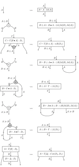
Our next goal is to show that we can also define proof nets inductively. We start with an inductive definition and proceed by showing that it in fact defines the whole class of proof nets. We use the notationN∗ for a net that should be drawn upside-down, i.e. mirrored vertically along an imaginary axis.

Definition 2.16(Proof Nets Inductively). The class of proof nets is defined inductively as follows:

• Identity. The identity proof net for arbitraryAis given by

(40)

• Composition. Given two proof nets

N1 A

B

and N2 B

C

the following is a proof net:

N1

N2 A

B

C

• Monotonicity. Given two proof nets

N1 A

C

and N2 B

D

the following are proof nets:

⊗

N1 N2

⊗

A⊗B

A B

C D

C⊗D

⇒

N₁∗ N2

⇒

C⇒B

C B

A D

A⇒D

⇐

N1 N₂∗

⇐

A⇐D

A D

C B

C⇐B

• Generalized Left Application. Given two proof nets

N1 A

C

and N2 B

(41)

⊗

N1 N2

⇒

A⊗B

A B

C C⇒D

D

• Generalized Right Application. Given two proof nets

N1 A

D⇐C

and N2 B

C

⊗

N1 N2

⇐

A⊗B

A B

D⇐C _C

D

• Generalized Left Co-Application. Given two proof nets

N1 C

A

and N2 A⊗B

D

(42)

⊗

N₁∗ N2

⇒

B A

A⊗B

C D

C⇒D

• Generalized Right Co-Application. Given two proof nets

N1 A⊗B

C

and N2 D

B

⊗

N1 N2∗

⇐

A

A⊗B

B

C D

C⇐D

• Generalized Left Lifting. Given two proof nets

N1 B

C

and N2 D

A⇒B

(43)

A⇒B

⇒

N1 N2∗

⇐

A

B

C D

C⇐D

• Generalized Right Lifting. Given two proof nets

N1 D

A⇐B

and N2 A

C

A⇐B

⇐

N∗

1 N2

⇒

B

A

C D

D⇒C

• Nothing else is a proof net.

Now we want to show that our inductive definition is correct, i.e. it defines precisely those proof structures that are proof nets. Before we prove this theorem, we need to show some additional properties of proof nets.

Property 2.1. Every proof structure has an equal number of tensor and cotensor nodes.

Proof. By definition, every proof structure has a unique input and a unique output. By well-formedness, an output of a link cannot be an input to the same link. Now, as each tensor node has 2 inputs and 1 output, and each cotensor node has 1 input and 2 outputs, this means that thein degree

(44)

nodes is 2n+m−(2m+n−1) =n−m+ 1 while theout degree isn+ 2m−(m+ 2n−1) =m−n+ 1. Now suppose thatn6=m. Then either the in or the out degree is 0 or less, which is impossible by the assumption that there is one unique input and one unique output. Hence,n=m.

Property 2.2. Every connected, well-typed graph made up from the given links has a directed path from any input to any output.

Proof. By induction on the number of nodes in a graph. The base case of zero nodes is trivial as the graph must consist of a single wire. For the inductive case, suppose that each graph withn

nodes has a directed path from any input to any output, and consider a proof structure withn+ 1 nodes. Now consider any input wire and any output wire. By connectedness, the input wire must enter some node. As every node has at least one output, consider the outputs of the node. If one of the outputs is the selected output wire, we are done. Otherwise proceed by considering one of the output wires of the node and proceed using the induction hypothesis.

Property 2.3 (Locality). For any proof net, each of its subgraphs with a unique in- and output, all correctness criteria hold, i.e. each of these subgraphs are proof nets as well.

Proof. Obviously, every subgraph of a proof net with a unique in- and output is a proof structure. It is also immediate that planarity and operator balance hold locally, since a violation of these in the subgraph would mean a violation in the whole graph. A similar reasoning holds for the return cycle requirement. Hence, we may conclude that the subgraph must be a proof net.

Theorem 2.2. A proof structure is a proof net if and only if it is generated by the inductive definition of proof nets.

Proof. The converse is easily shown by inspecting the generating rules and seeing that they preserve operator balance and the return cycle requirement. For the left to right direction, things are more difficult. We proceed by induction on the number of nodes. As proof nets have an equal number of tensor and cotensor nodes, we will try to show that we can take off one tensor and one cotensor node at a time to proceed with the induction hypothesis. The base case is trivial, as it can only be a proof net consisting of a single wire, which is also the base case of the inductive definition. For the inductive case, suppose that any proof net with up tonnodes can be inductively generated, and consider a proof netN withn+ 2 nodes. First of all, because of the external face requirement, we can always identify atop node and abottom nodeas outermost nodes of the proof net. Secondly we note that a proof net cannot have as top node (i.e. the node with the unique loose input wire) the following two links:

⇒

A B

A⇒B

⇐

B A

B ⇐A

(45)

⊗

A⊗B

A B

This is because, by property 2.2, there will always be a path from the outputs of this link, back to the node, and hence the return cycle requirement will be violated.

We will now proceed by case distinction considering different cases whereNstarts with a certain link and ends with a certain link (although there are a lot of cases to go through, we will treat them systematically):

1. The case whereN starts with a cotensor node and ends with a tensor node: soN is of one of the following forms:

⊗

N0

⊗

A⊗B

C⊗D

⊗

N0

⇒

A⊗B

C⇒D

⊗

N0

⇐

A⊗B

D⇐C

In this case, we claim thatN is either composite or actually of the form

⊗

N1 N2

⊗

A⊗B

A B

C D

C⊗D

⊗

N1 N2

⇒

A⊗B

A B

C

D

C⇒D

⊗

N1 N2

⇐

A⊗B

A B

D

C

D⇐C

whereN1 andN2 are proof nets.

MoL 2014 22: Categorical Foundations for Extended Compositional Distributional Models of Meaning

Categorical Foundations for Extended Compositional Distributional

Models of Meaning

MSc Thesis

(Afstudeerscriptie)

MSc in Logic

Acknowledgements

Contents

I

Basic Compositional Distributional Models of Meaning

14

II

Extended Compositional Distributional Models of Meaning

90

Introduction

Compositionality and Type-Logical Grammar

A Classic: the CHL Correspondence

Graphical Reasoning in Logic and Categories

Recap: Problem Statement in Context

What This Thesis is Not About

Overview of Type-Logics

Contributions and Structure of the Thesis

Part I

Chapter 1

Categories

1.1

The Basics

1.2

Monoidal and Closed Categories

1.3

Monoidal and Closed Functors

1.4

Symmetry

Chapter 2

Graphical Languages

2.1

Graphical Languages: an Introduction

2.2

Graphical Languages for Monoidal Categories

2.2.1

Going Monoidal

2.2.2

Closing the Category

2.2.3

A Problem With the Clasp Language

2.3

Graphical Languages for Closed Tensor Categories

2.3.1

Proof Nets versus Graphical Languages

2.3.2

Signatures, Interpretations and Free Categories

2.3.3

Sequent Calculus Categorified

2.3.4

Proof Nets Defined