Spatial Resolution of Satellite Data
Using the Maximum Entropy Method
by
Christopher James Jackett, B.Sc. (Hons)
A dissertation submitted in fulfilment of the requirements for the
degree of Doctor of Philosophy in the CSIRO-UTAS PhD Program
in Quantitative Marine Science
School of Computing and Information Systems
University of Tasmania
This thesis contains no material which has been accepted for a degree or diploma by
the University or any other institution, except by way of background information
and duly acknowledged in the thesis, and to the best of my knowledge and belief
no material previously published or written by another person except where due
acknowledgement is made in the text of the thesis, nor does the thesis contain any
material that infringes copyright.
Signed: Date:
Christopher James Jackett PhD Candidate
Computing and Information Systems
University of Tasmania
This thesis may be made available for loan. Copying and communication of any part
of this thesis is prohibited for two years from the date this statement was signed;
after that time limited copying and communication is permitted in accordance with
the Copyright Act 1968.
Signed: Date:
Christopher James Jackett PhD Candidate
Computing and Information Systems
University of Tasmania
The following publication contributed to the work undertaken as part of this thesis:
Jackett, C. J., Turner, P. J., Lovell, J. L., Williams, R. N., ‘Deconvolution
of MODIS imagery using multiscale maximum entropy’, Remote Sensing
Letters, Volume 2, No. 3, September 2011, Pages 179-187
C. J. Jackett was the primary author (70%). He performed the majority of the
experimental work and subsequent analysis. P. J. Turner (12%) and J. L. Lovell
(12%) helped guide the development and assisted in the analysis. R. N. Williams
(6%) provided general support and advice. All authors provided feedback and
suggestions on the manuscript.
We the undersigned agree with the above stated proportion of work undertaken for
the above published manuscript contributing to this thesis.
Signed:
Christopher James Jackett Dr. Robert Bruce Ollington
PhD Candidate Primary Supervisor
Computing and Information Systems Computing and Information Systems
University of Tasmania University of Tasmania
Date:
Remote sensing satellite imagery provides information about the surface of the Earth
at a range of spectral bands and spatial resolutions. This information is a valuable
resource for the management of terrestrial and marine environments. During the
capturing process, incoming light is reflected or refracted by the instrument optics
which causes a small amount of blurring. This effect is described by a mathematical
operation called convolution in which the satellite input radiance field is convolved
with the instrument Point Spread Function (PSF). This form of instrumental
distortion has the largest impact on high-contrast scenes where bright land or clouds
are adjacent to dark surfaces such as water.
This thesis investigates three mechanisms for improving the quality of recorded
satellite data. An efficient convolution method was developed to minimise boundary
effects, a deconvolution algorithm was used to remove instrumental distortion,
and a resolution enhancement algorithm was developed to improve the spatial
resolution of input images. The latter two of these problems are underdetermined
and require appropriately selected constraints in order to find unique and stable
solutions. An entropy-based method was chosen as the constraint element due to
its heavy grounding in statistical mechanics and information theory. MODerate
resolution Imaging Spectroradiometer (MODIS) Aqua images were used to quantify
the improvement of these algorithms, with a focus on coastal marine and open-ocean
environments.
Deconvolution is an algorithm-based process designed to reverse convolution
effects with a known PSF. Multiscale Entropy deconvolution was applied to MODIS
level 1A imagery to remove instrumental distortion from top-of-atmosphere radiance
counts. Removing these effects at the beginning of the satellite image processing
stages. Wavelet transforms were implemented to decompose images into a range
of resolution levels that represent different spatial frequencies. This allows both
large-scale and small-scale features to be resolved simultaneously. Multiresolution
Support images were used to accurately define and target important areas within the
imagery. The combination of these techniques includes two-dimensional structural
information in the Multiscale Entropy calculation which results in accurate
deconvolution. Validation of the Multiscale Entropy deconvolution algorithm was
undertaken using in-situ measurements from the Baltic Sea and a QuickBird image
of a high-contrast Antarctic ice edge.
A novel approach to the spatial resolution enhancement of MODIS imagery
uses information about the optical PSF, along with the result of Multiscale
Entropy deconvolution. With this information, a system of linear equations
was constructed that models how high-resolution PSF convolution redistributes
information over a finite area. A new method termed Multiresolution Entropy
was developed to constrain the linear system and retrieve an optimal solution.
The algorithm successfully improved the spatial resolution of input images and
compared favourably to other interpolation-based methods. The key requirement of
this technique is to obtain high-resolution PSF measurements at the same sampling
frequency as the desired final output resolution.
The techniques developed and presented in this thesis contain a range of
important research contributions. The combination of Fast Fourier Transform
convolution with a boundary renormalisation approach produces an efficient and
accurate convolution method with minimal boundary effects. A multi-detector
convolution process accurately simulates the MODIS Aqua instrumentation and
allows for successful deconvolution. A detector saturated estimation technique
for ocean colour bands ensures the correct quantity of instrumental distortion is
removed during deconvolution. The formulation of a linear system consisting of
high-resolution PSF modelling and appropriate physical constraints defines the spatial
resolution enhancement problem. The development of Multiresolution Entropy
targets high-frequency content, constrains the linear system and results in a unique
thesis provide considerable benefit to the quality of remote sensing imagery and can
substantially improve the monitoring and management of coastal zones and other
marine environments.
I would like to thank Jenny Lovell and Robert Ollington for supervising this thesis.
Their dedicated guidance and support was gratefully appreciated. Ray Williams and
Peter Turner are also acknowledged for their supervision efforts in the early stages
of this research. I would particularly like to thank Peter Turner for providing the
initial inspiration for this work and outlining a worthwhile and rewarding research
topic.
My gratitude extends to Thomas Schroeder, Young Je Park, Ian Grant and
Edward King for reading draft manuscripts and providing useful feedback. Edward
King also receives my appreciation for processing a range of MODIS scenes.
Gerhard Meister, Jack Xiong and Brian Wenny generously provided the MODIS
Aqua characterisation models that underpin many of the research components in
this thesis. I would like to thank Susanne Kratzer for providing in-situ Baltic
Sea validation measurements and making suggestions regarding the deconvolution
algorithm validation. Selima Ben Mustapha and Gerald More helped facilitate the
direct comparison of in-situ Baltic Sea and MODIS measurements. Petra Heil also
provided high-resolution QuickBird validation data.
Finally, a special thank you to my wife Amy Jackett for always listening to my
current problems, suggesting alternative strategies and being incredibly supportive.
Declaration i
Authority of Access ii
Statement of Co-authorship iii
Abstract iv
Acknowledgements vii
1 Introduction 1
2 Background 7
2.1 MODIS Aqua . . . 7
2.2 Convolution . . . 9
2.3 Deconvolution . . . 22
2.3.1 Linear Regularisation Methods . . . 24
2.3.2 CLEAN . . . 27
2.3.3 Bayesian Methods . . . 29
2.3.4 Maximum Entropy Method . . . 31
2.4 Resolution Enhancement . . . 35
3 Convolution 38 3.1 Introduction . . . 38
3.2 Method . . . 45
3.3 Results . . . 48
4 Deconvolution 57
4.1 Introduction . . . 57
4.2 MODIS Aqua PSF . . . 58
4.3 Multiscale Entropy Deconvolution . . . 63
4.4 Results . . . 81
4.5 Summary . . . 91
5 Validation 92 5.1 Introduction . . . 92
5.2 In-situ Baltic Sea . . . 95
5.2.1 Method . . . 95
5.2.2 Results . . . 102
5.3 QuickBird Southern Ocean . . . 110
5.3.1 Method . . . 110
5.3.2 Results . . . 118
5.4 Summary . . . 122
6 Spatial Resolution Enhancement 124 6.1 Introduction . . . 124
6.2 Problem Formulation . . . 127
6.3 Linear System Regularisation . . . 137
6.4 Results . . . 150
6.4.1 Solution Quality Analysis . . . 178
6.4.2 Gradient Step Size . . . 179
6.4.3 Computational Complexity . . . 181
6.4.4 PSF Structure . . . 183
6.4.5 Signal-to-Noise Ratio Analysis . . . 185
6.4.6 Varied Resolution Enhancement Factors . . . 185
6.4.7 Future Work . . . 190
7 Conclusion 194
7.1 Research Contribution . . . 195
7.2 Summary of Results . . . 196
2.1 MODIS Aqua cutaway detailing the MODIS scan cavity subsystems
and on-board calibrators (Xiong et al., 2005). . . 8
2.2 Two-dimensional representations of (a) the convolution kernel, (b)
the data to be convolved and (c) the convolution of the first data
point with the convolution kernel. . . 11
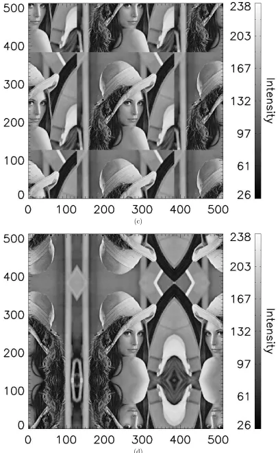
2.3 Common boundary conditions added to standard image processing
test image Lena (256×256) including (a) zero-padding and (b)
repetition. . . 13
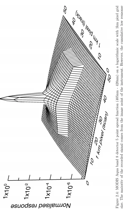
2.4 MODIS Aqua band 8 detector 5 point spread function (405nm
-420nm) on a logarithmic scale with 1km pixel grid size. . . 16
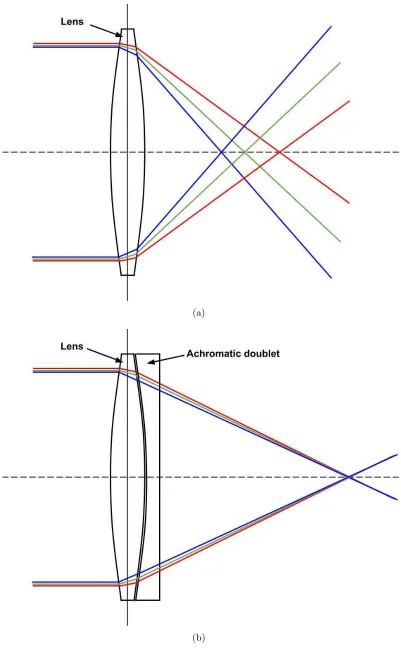
2.5 Refraction of light wavelengths through an optical lens showing (a)
chromatic aberration and (b) a correction technique called achromatic
lensing. . . 18
2.6 Images from Hubble’s Wide Field and Planetary Camera (WFPC) of
spiral galaxy M100 showing (a) the uncorrected image with spherical
aberration and (b) the image after corrected optics were applied
(NASA, 1993). . . 19
2.7 Airy pattern instrument response caused by the diffraction of light
through a uniformly illuminated circular aperture. . . 20
3.1 Computational advantage of FFT convolution over standard
convolution. . . 42
3.2 Padded convolution efficiency threshold above which it is faster to
perform FFT convolution and below which it is faster to perform
standard convolution. . . 43
3.3 Boundary contamination encountered by convolving a zero-padded
flat signal (length = 300, value = 1.0) with a normalised symmetrical
Gaussian convolution kernel (length = 155, FWHM = 77). . . 44
3.4 Linearly increasing signal (length = 300) with zero-padding,
replication, mirroring and repetition boundary conditions (length
= 150) depicted beyond the limits of the original signal. . . 46
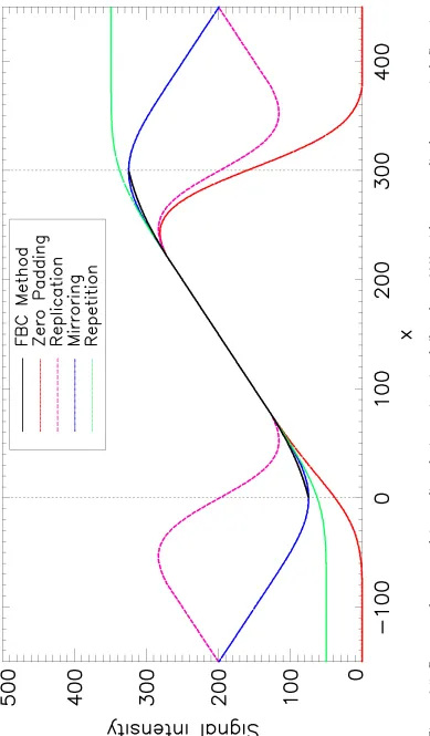
3.5 Response from convolving a linearly increasing signal (length = 300)
with a normalised symmetrical Gaussian convolution kernel (length
= 155, FWHM = 77) using zero-padding, replication, mirroring,
repetition boundary conditions and the FBC method. . . 49
3.6 One-dimensional test signals used to test the equivalence of the FBC
and SBR methods including (a) a one-dimensional flat line and (b) a
one-dimensional sine wave. . . 51
4.1 MODIS Aqua band 8 point spread functions (405nm - 420nm) on a
logarithmic scale with 1km pixel grid size including (a) detector 1,
(b) detector 5 and (c) detector 10. . . 59
4.2 Contamination test showing (a) synthetic test scene with typical
land and ocean reflectance, (b) synthetic test scene convolved with
MODIS Aqua band 8 PSF with original boundary indicated and (c)
comparison of original (solid) and convolved (dashed) right-hand edge
transects. . . 61
4.3 Relative contamination error caused by MODIS Aqua band 8 PSF
on synthetic test scene (Figure 4.2(a)) with varying land/cloud
reflectance levels. . . 62
4.4 Multiresolution Wavelet decomposition depicting (a) the original test
image ‘Lena’ and (b) the first Wavelet scale containing high-frequency
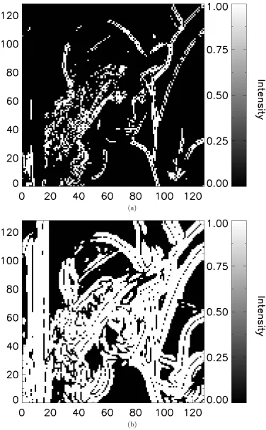
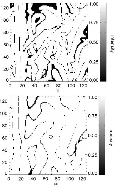
4.5 Multiresolution Support images calculated from the Wavelet
decomposition of Figure 4.4(a) showing (a) level 1 support containing
high-frequency content and (b) level 2 support containing moderately
high-frequency content. . . 71
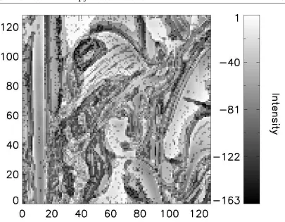
4.6 Visualisation of the Multiscale Entropy on Figure 4.4(a). . . 74
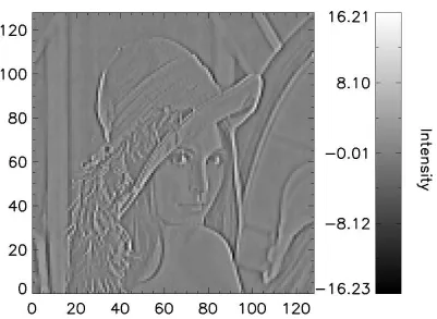
4.7 First iteration search direction for the Multiscale Entropy
deconvolution of Figure 4.4(a). . . 76
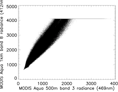
4.8 Scatter plot of 500m resolution MODIS Aqua band 3 (469nm) with
1km resolution MODIS Aqua band 8 (412nm) for a typical MODIS
Aqua scene containing a range of water, land and cloud measurements. 78
4.9 Scatter plot of 500m resolution MODIS Aqua band 3 (469nm) with
1km resolution MODIS Aqua band 8 (412nm) for a typical MODIS
Aqua scene with filtered saturated measurements. . . 80
4.10 Scatter plot of 500m resolution MODIS Aqua band 3 (469nm) with
1km resolution MODIS Aqua band 8 (412nm) for a typical MODIS
Aqua scene with estimated saturated measurements. . . 80
4.11 Synthetic data deconvolution accuracy test showing (a) the original
image and (b) the original image convolved with MODIS Aqua band
8 PSF and average band 8 noise added. . . 82
4.12 MODIS deconvolution test showing (a) the original MODIS Aqua
band 12 data (convolved and noisy) and (b) the deconvolved MODIS
Aqua band 12 data. . . 86
4.13 MODIS deconvolution test showing (a) the original MODIS Aqua
band 12 data (convolved and noisy) and (b) the deconvolved MODIS
Aqua band 12 data. . . 89
5.1 In-situ measurement stations for the July 2008 sea-truthing campaign. 96
5.2 MODIS Aqua true-colour images for full Baltic Sea overpasses on (a)
24/07/2008, (b) 25/07/2008 and (c) 31/07/2008. . . 98
5.3 Typical Baltic Sea reflectance spectra for increasing quantities of
5.4 Spectral reflectance curve showing an underlying amplified typical
Baltic Sea reflectance spectrum (black crosses), fitted curve weighted
by in-situ measurements 50:1 (red line), in-situ measurements (blue
crosses) and MODIS-compatible measurements drawn from the fitted
curve (green crosses). . . 101
5.5 Direct comparison of in-situ remote sensing reflectance spectra
with MODIS reflectance spectra before and after deconvolution for
sampling stations BI and BII on 24/07/2008. . . 103
5.6 Direct comparison of in-situ remote sensing reflectance spectra
with MODIS reflectance spectra before and after deconvolution for
sampling stations BIII and BY31 on 24/07/2008. . . 104
5.7 Individual band scatter-plot comparisons of in-situ and MODIS
remote sensing reflectance measurements before and after
deconvolution for the 2008 sea-truthing campaign (Kratzer and
Vinterhav, 2010). . . 105
5.8 Comparisons of in-situ sea-truth and MODIS Aqua
chlorophyll-a concentrchlorophyll-ation (GSM), Totchlorophyll-al Suspended Mchlorophyll-atter (TSM) chlorophyll-and the
spectral diffuse attenuation coefficient (Kd(490)) before and after
deconvolution for the 2008 sea-truthing campaign (Kratzer and
Vinterhav, 2010). . . 107
5.9 QuickBird RGB true-colour image featuring an Antarctic ice edge. . . 112
5.10 Locations of MODIS Aqua data points depicted on top of the
QuickBird area of interest subset. . . 114
5.11 Locations and spatial coverage of the final MODIS Aqua pixels
showing averaged QuickBird intensities depicted on top of the
QuickBird area of interest for the blue-band. . . 116
5.12 Relative spectral response of blue, green and red QuickBird channels
and the 6 associated MODIS Aqua bands. . . 117
5.13 Comparison of MODIS Aqua original and deconvolved data points
5.14 Comparison of MODIS Aqua original and deconvolved data points
with down-sampled QuickBird measurements for the green wavelengths.120
5.15 Comparison of MODIS Aqua original and deconvolved data points
with down-sampled QuickBird measurements for the red wavelengths. 121
6.1 Two-dimensional representations of (a) the original recorded image
I (5×5), (b) the nearest-neighbour interpolation of O (5×5) producing ↑O (10×10), and (c) a high-resolution point spread function (3×3) sampled at the same frequency as ↑O. . . 130 6.2 Two-dimensional representations of (a), (b), (c) and (d) the four point
convolutions at high resolution that make up the equivalent single
lower-resolution point convolution and (e) the composite convolution
achieved by spatially combining the four individual point convolutions
in (a), (b), (c) and (d). . . 131
6.3 One-dimensional representations of (a), (b), (c) and (d) the four
point convolutions including only overlapping data points in ↑O and (e) the composite convolution achieved by spatially combining and
renormalising the four individual point convolutions. . . 132
6.4 Two-dimensional representations of the complete convolution of ↑O
with↑Pc showing (a), (b), (c), (d) and (e) composite individual
high-resolution point convolutions and (f), (g), (h) and (i) five combined
composite individual high-resolution point convolutions. . . 134
6.5 One-dimensional representation of the cumulative construction of the
linear system with (a) corresponding to Figures 6.4(a), 6.4(b), 6.4(c),
6.4(d) and 6.4(e), and (b), (c), (d) and (e) corresponding to Figures
6.4(f), 6.4(g), 6.4(h) and 6.4(i) respectively. . . 135
6.6 One-dimensional representation of the complete linear system
including a power-conserving constraint. . . 137
6.7 Multiresolution Support decomposition of (a) original standard test
6.8 Logarithmically rescaled Multiresolution Entropy response to
standard test image ‘Lena’ (Figure 6.7(a)) showing large quantities
of entropy in regions of high-frequency content. . . 148
6.9 Multiresolution Entropy gradient response to standard test image
‘Lena’ (Figure 6.7(a)) showing the initial MRE search direction for
the linear system. . . 148
6.10 Flowchart describing the experimental design procedure for
processing synthetic test images, enhancing spatial resolution and
comparing the results. . . 151
6.11 Resolution enhancement evaluation procedure showing (a) the
high-resolution truth image (64×64) and(b) the low-resolution convolved
and noisy image (32×32). . . 155
6.12 MERE results showing (a) the spatially enhanced image (64×64) and
(b) the difference between the MERE result and the high-resolution
truth image (64×64). . . 157
6.13 Bilinear interpolation results showing (a) the bilinearly enhanced
image (64×64) and (b) the difference between the bilinear result
and the high-resolution truth image (64×64). . . 159
6.14 Tikhonov resolution enhancement results showing (a) the Tikhonov
enhanced image (64×64) and (b) the difference between the
Tikhonov result and the high-resolution truth image (64×64). . . 162
6.15 Bicubic interpolation results showing (a) the bicubic interpolation
enhanced image (64×64) and (b) the difference between the bicubic
result and the high-resolution truth image (64×64). . . 164
6.16 Test images showing (a) a standard USC texture mosaic #2
comprising various sized blocks of uniform intensity and (b) a
standard USC texture mosaic #3 comprising more complicated
regions of uniform intensity. . . 167
6.17 Resolution-enhanced result comparison for USC texture mosaic #2
(Figure 6.16(a)) showing (a) the MERE reconstructed result and (b)
6.18 Resolution-enhanced result comparison for USC texture mosaic #3
(Figure 6.16(b)) showing (a) the MERE reconstructed result and (b)
the bilinearly interpolated result. . . 171
6.19 Resolution-enhanced result comparison for standard airport test
image (Figure 6.16(c)) showing (a) the MERE reconstructed result
and (b) the bilinearly interpolated result. . . 174
6.20 Resolution-enhanced result comparison for MODIS test image (Figure
6.16(d)) showing (a) the MERE reconstructed result and (b) the
bilinearly interpolated result. . . 176
6.21 Gradient step size, γ, at each iteration of the MERE algorithm. . . . 180 6.22 Resolution-enhanced reconstruction error calculated using the
Euclidean difference norm method as a function of PSF FWHM. . . . 184
6.23 Resolution-enhanced reconstruction error calculated using the
Euclidean difference norm method as a function of detector-based
SNR. . . 186
6.24 Resolution-enhanced reconstruction error calculated using the
Euclidean difference norm method as a function of the resolution
enhancement factor. . . 186
6.25 Resolution-enhanced reconstructions with resolution enhancement
factors of (a) 2, (b) 3 and (c) 4 using the MERE algorithm. . . 188
6.26 Resolution-enhanced reconstructions with resolution enhancement
3.1 All test signals are convolved with both the FBC and SBR methods. 54
4.1 Spectrally matched band combinations of the MODIS ocean colour
and high-resolution land/cloud bands. . . 79
5.1 Sampling stations, sampling times and MODIS overpass times for the
July 2008 sea-truthing campaign. . . 97
5.2 MNB and RMS results for remote sensing reflectance,
chlorophyll-a, TSM and Kd(490) for original and deconvolved MODIS Aqua
measurements. . . 109
6.1 Reconstruction errors calculated using the Euclidean difference norm
method for each test image and resolution enhancement method. . . . 178
6.2 Structural similarity index values calculated for each test image and
resolution enhancement method. . . 180
6.3 Computational complexities of nearest-neighbour, bilinear, bicubic
convolution and bicubic spline image resamplings of an n×n pixel image. . . 181
6.4 Computational complexities of the components required to enhance
spatial resolution using MERE and Tikhonov resolution enhancement. 182
ABS Australian Bureau of Statistics
AERONET-OC AErosol Robotic NETwork Ocean Colour
AVHRR Advanced High Resolution Radiometer
BB Barzilai and Borwein method
CDOM Coloured Dissolved Organic Matter
CUDA Compute Unified Device Architecture
DFT Discrete Fourier Transform
DSP Digital Signal Processing
EOS Earth Observing System
FBC Fast Fourier Transform with Border Correction
FFT Fast Fourier Transform
FWHM Full-Width Half-Maximum
GCV Generalised Cross-Validation
HR High Resolution
HST Hubble Space Telescope
IDL Interactive Data Language
LR Low Resolution
MAP Maximum A Posteriori
MEM Maximum Entropy Method
MERE Maximum Entropy Resolution Enhancement
MERIS MEdium Resolution Imaging Spectrometer
MLS Method of Least Squares
MNB Mean Norm Bias
MODIS MODerate resolution Imaging Spectoradiometer
MRE MultiResolution Entropy
PSF Point Spread Function
REF Resolution Enhancement Factor
RMS Root Mean Square
SBAF Spectral Band Adjustment Factor
SBR Standard Convolution with Boundary Renormalisation
SeaDAS SeaWiFS Data Analysis System
SNR Signal-to-Noise Ratio
SSIM Structural SIMilarity
SVD Singular Value Decomposition
TSM Total Suspended Matter
USGS U.S. Geological Survey
VHR Very High Resolution
Introduction
Monitoring marine environments is critical to the sustainable management of coastal
regions and resources. Approximately 85% of the Australian population live within
50km of the coastline, of which a large proportion live in state capital cities
that are located on or near the coast (Australian Bureau of Statistics, 2002).
These regions are constantly subjected to pressure from recreational and industrial
fishing, coastal population growth and urbanisation, storm water run-off, human
waste management, anthropogenic climate change, and large-scale natural events
including flooding, fires and other weather-related phenomena. Therefore, it is
crucial to develop accurate monitoring systems that deliver frequent, high-resolution
information to help manage these densely populated regions.
Remote sensing is the attainment of information about objects with which the
observer has no physical contact. Remote sensing enables data to be collected
in areas previously unavailable due to cost, inaccessibility or danger (Ikeda and
Dobson, 1995). One form of remote sensing uses artificial Earth-orbiting satellites
to record data about the surface of the Earth. Highly-sensitive satellite instruments
can accurately record information about the Earth, from which products such as sea
surface temperature, ocean colour, vegetation indices and global solar radiation can
be derived (Baker, 1990). Some commonly used remote sensing satellite instruments
include the Advanced Very High Resolution Radiometer (AVHRR) (km resolution),
which senses cloud cover, surface brightness and surface temperature (NOAA,
2010); the MODerate resolution Imaging Spectroradiometer (MODIS) (250m - 1km
resolution), which measures large scale global dynamics (Justice et al., 1998); and
the Landsat Thematic Mapper (30m - 100m resolution), which is a multi-spectral
scanning radiometer used to detect and measure changes on the surface of the
Earth (USGS, 2009). Other higher-resolution instruments capture spatially detailed
information at less frequent time intervals or in targeted data acquisitions.
This thesis will concentrate on MODIS satellite instruments on-board the Earth
Observing System (EOS) platform Aqua. MODIS Aqua captures data in 36 spectral
bands at several spatial resolutions including 250m, 500m and 1km resolution.
MODIS Aqua is calibrated to deliver over 40 standard data products such as
atmospheric aerosols, snow cover, land and water surface temperature, leaf area
index, sea ice extent and ocean chlorophyll concentration among many others. Aqua
is fixed in a sun-synchronous, near-polar, circular orbit designed to maintain an
equatorial crossing at approximately 10:30 A.M. local time each day. Aqua travels
at a forward velocity of approximately 7.5km/s in low Earth orbit at an altitude of
705km. This rapid orbital path allows MODIS to provide complete global coverage
every one to two days.
MODIS Aqua measures top-of-atmosphere radiance counts by reflecting the
Earth-leaving light field onto an array of detectors using a rotating
double-sided mirror. As the light field interacts with the instrument optics, a small
amount of blurring is introduced into the recorded signal. This blurring is an
inherent property of all sensor-based optical systems and is described by the
mathematical operation known as convolution. That is, the existing
distortion-free light field enters the instrument and becomes convolved with the instrumental
spatial response function. The optical system introduces spatial distortion and
attenuates the signal. The signal is then detected by sensors which add noise
and have their own intrinsic gain characteristics. Calibrating the entire system to
make an accurate measure of radiance is a critical issue and has been achieved by
Guenther and Barnes (1996) and Xiong and Barnes (2006). Given the calibration
process has been performed successfully, a correction for optical distortion can be
made. Deconvolution algorithms are designed to retrieve the optimal distortion-free
characterised. Detector-based noise is the primary factor that makes deconvolution
problems ill-posed and difficult to solve. However, a unique and stable solution can be
found by applying a suitable set of constraints. This thesis investigates the Multiscale
Entropy deconvolution of MODIS Aqua data to accurately remove instrumental
distortion and improve satellite imagery. Light detection and instrumental distortion
are the last processes to occur in the light-path of the recorded signal and should
therefore be the first effects that are corrected. Removing instrumental distortion
errors directly after detector calibration limits the amplification of these errors at
subsequent processing stages. This is a core argument that is central to the satellite
image deconvolution research described in this thesis.
The convolution operator is one of the fundamental calculations performed within
every iteration of the deconvolution process. Selecting the appropriate convolution
boundary condition is a major concern for successful image deconvolution. A
common approach is to add a zero-padded border around the convolution input
image, and remove the border immediately after convolution is performed. However,
image content that is redistributed into the padded border is removed with every
iteration of the deconvolution algorithm, resulting in a spatially biased loss of
image intensity. Fast Fourier Transforms (FFTs) are commonly applied to increase
the computational speed of convolution. In this thesis, a new convolution method
will be developed that combines the speed benefits attributed to FFT convolution
with a boundary renormalisation approach to provide efficient and robust signal
convolution.
Image spatial resolution is a fundamental measure of image quality. Methods
designed to preserve or enhance spatial resolution are considered highly valuable.
The natural instrumental convolution that occurs during satellite measurements
is an analogue process that redistributes image content over a finite area. Using
this knowledge, it is possible to improve the spatial resolution of a recorded
image that has undergone a natural convolution process, provided that a
high-resolution instrument response function is available. This thesis investigates an
entirely novel approach to spatial resolution enhancement using high-resolution
method.
The data collecting capabilities provided by MODIS Aqua, and other remote
sensing platforms, allow for constant and accurate monitoring of both coastal marine
and open-ocean environments. This information has remarkable value, and any
improvements made to the data processing chain are highly advantageous. This
thesis aims to identify, explore, quantify and correct three distinct mechanisms
that occur in the retrieval and processing of satellite imagery. These mechanisms
include an efficient convolution correction method that can minimise boundary
contamination, an operational image deconvolution algorithm implemented for
MODIS Aqua ocean colour bands, and a novel spatial resolution enhancement
method for optical imaging systems. These three research components will be
investigated and developed with the aim of improving the monitoring and
management of coastal marine and open-ocean environments.
All of the computational techniques developed throughout this thesis are
implemented in the Interactive Data Language (IDL). IDL was selected because it
contains a rich base of mathematical libraries that are fundamental to the algorithms
developed in this thesis, and IDL is a standard programming language in the remote
sensing research field.
Chapter 2 introduces relevant literature and background information concerning
the three main research areas. A comprehensive review of current techniques and
their limitations is explored and the necessity for further research and development
is highlighted. The specific techniques developed in this thesis are general and have
a wide range of application in other fields.
Chapter 3 describes a correction method for FFT convolution that limits
boundary contamination artefacts resulting from convolution padding methods.
The proposed correction method makes a single data-driven boundary condition
assumption and only uses information contained within the original input signal
to produce consistent convolution results and maintain data integrity. An analysis
of the algorithm shows that it performs identically to the equivalent spatial-domain
convolution approach with the only discernible differences being resolved at the level
to performance and has valuable applications for scientific data processing where
algorithm efficiency and data accuracy are imperative.
Chapter 4 investigates the Multiscale Entropy deconvolution of MODIS Aqua
imagery which results in the removal of instrument response function effects. The
implementation utilises three efficient computational methods: FFT convolution,
Wavelet image decomposition and a gradient method step size estimation algorithm
that together enable rapid image deconvolution. Multiscale Entropy uses Wavelet
transforms to implicitly include two-dimensional structural information of an image
into the entropy calculation. An evaluation using synthetic data showed that the
deconvolution algorithm reduced the maximum individual pixel error from 90.01%
to 0.34%, effectively removing instrumental distortion down to the level of
detector-based noise. Deconvolution of MODIS data is shown to resolve all significant features
and is most effective in regions with large changes in radiance such as coastal zones,
contrasting land covers and cloud edges.
Chapter 5 describes the validation process of the Multiscale Entropy
deconvolution of MODIS Aqua imagery using two separate validation approaches.
In-situ Baltic Sea samples including surface reflectance, chlorophyll-a, total
suspended matter and the diffuse attenuation coefficient were compared with
MODIS Aqua overpass measurements. However, minimal scene contrast and
limited in-situ spatial extent were found to insufficiently characterise the effects of
deconvolution. A high-resolution QuickBird scene containing an Antarctic ice edge
was spatially matched and directly compared with MODIS Aqua top-of-atmosphere
radiance measurements. The results indicate that deconvolution improved the
radiometric accuracy of MODIS Aqua measurements in the blue wavelengths, but
did not contain a sufficient number of comparable measurements in the green or red
wavelengths to reach any strong conclusions.
Chapter 6 develops a novel spatial resolution enhancement technique for satellite
imagery by using high-resolution instrument response function measurements and
pre-processed image deconvolution results. The resolution enhancement problem
is formulated as an ill-posed system of linear equations by modelling a
ill-posed inverse problem can be solved using a novel variant of Multiscale Entropy
regularisation, which is designed to simultaneously maximise information content
and manage detector-based noise. This technique shows particular promise for
single-frame imagery. Results show that this approach can moderately enhance the spatial
resolution of satellite imagery, provided the instrument response function is sampled
at the desired final resolution-enhanced sampling frequency.
Chapter 7 summarises each of the major research components in this thesis
and discusses their original contribution. The improvement that each research
topic contributes to satellite data is outlined and its impact on the monitoring
and management of coastal marine and open-ocean environments is discussed.
Concluding remarks for each research component are presented and an evaluation
Background
2.1
MODIS Aqua
Containing six Earth-observing instruments, Aqua was launched on May 4, 2002
to observe and study the water cycle. The main instrumentation inside MODIS
Aqua comprises a double-sided scan mirror that continuously rotates and reflects
Earth-leaving radiances onto an along-track array of detectors (Figure 2.1). As the
scanning mirror rotates, MODIS Aqua horizontally stripes the surface of the Earth
in the scan direction while the craft travels forward in the track direction (Barnes
et al., 1998). These strips of data are combined to build up a continuous image.
MODIS Aqua contains a field baffle that restricts the input radiance field to a 10km
field-of-view in the along-track dimension. This enables a 10-element scan to be
recorded across the swath for each 1km resolution band. Similarly, the 500m and
250m resolution bands record 20 and 40-element arrays respectively. The field baffle
has a strong effect on the instrument response. The spatial response of each detector
in every band has a unique shape determined by the relative position of the detector
with respect to the field baffle.
MODIS Aqua has a zenith angle of±55◦
and achieves a swath width of 2330km.
This translates to an unprocessed image width of 1354 pixels at 1km resolution due
to the range of viewing angles of the instrument and the curvature of the Earth. The
imagery retrieved from MODIS Aqua is segmented into individual datasets known as
granules. Each granule consists of 5 minutes satellite time of recorded imagery and
Figure 2.1: MODIS Aqua cutaway detailing the MODIS scan cavity subsystems and on-board calibrators (Xiong et al., 2005).
results in a final unprocessed image size of 1354×2040 pixels at 1km resolution.
This level 0 data contains raw digital number readings from the instrument and
are processed into level 1A radiance counts using NASA’s SeaWiFS Data Analysis
System (SeaDAS) (Fu et al., 1998; Nishihama et al., 1997). Processing the imagery
to level 1B adds calibration and geolocation information to the imagery (Xiong et al.,
2005). Further processing to level 2 or 3 results in individual data products, such as
sea surface temperature or ocean colour, which are readily used in many scientific
research fields.
The scanning-based design of MODIS Aqua results in the spatial coverage of
recorded measurements increasing in both the scan and track dimensions as the
instrument zenith angle increases. As the spatial coverage of MODIS measurements
grow at large zenith angles, the spatial pattern of the scan takes on the shape of a
bow-tie. This results in the spatial coverage of consecutive scans partially overlapping
at off-nadir angles, and is known as the panoramic bow-tie effect. When MODIS data
is reprojected to produce standard data products, intelligent measurement selection
schemes are employed to account for these effects. Spatially duplicate measurements
2.2
Convolution
Convolution is a mathematical process which combines two input signals to produce
a third resultant output signal. Each value in the convolved output signal is equal
to the sum of the point-wise multiplication of the two overlapping input signals.
The first input signal is typically the data to be convolved and the second input
signal is often referred to as the convolution function, impulse response function,
point spread function, blurring kernel or filter kernel. Convolution is often described
as the single most important technique in Digital Signal Processing (DSP) and
has many applications in other fields including electrical engineering, statistics and
probability (Smith, 2003; J¨ahne, 2002; Acharya and Ray, 2005). For a continuous
system, the convolution of two signals, f and g, is described using the convolution integral (Smith, 2003):
(f ∗g)(x) =
Z ∞ −∞
f(u)g(x−u) du (2.1)
where ∗ is the convolution operator
Discrete signals are required for digital computation to be performed. The
equivalent convolution operation can be represented for discrete systems using the
convolution sum (Smith, 2003):
O(x) = (I∗K)(x) =
M−1
X
i=0
K(i)I(x−i) (2.2)
where O(x) = convolved output signal (N+M −1 elements)
I(x) = input signal (N elements)
K(x) = convolution kernel (M elements)
the point-wise multiplication of the two signals to produce the final convolved signal.
The following mathematical properties hold for convolution (J¨ahne, 2002):
Commutativity f∗g = g∗f
Associativity f1∗(f2∗g) = (f1∗f2)∗g
Distributivity over Addition (f1+f2)∗g = f1∗g+f2∗g
There are many applications that require convolution to be performed on
two-dimensional imagery. For this purpose, Equation 2.2 can easily be extended into
two-dimensional space for use in image convolution:
O(x, y) =
M−1
X
j=0
M−1
X
i=0
K(i, j)I(x−i, y−j) (2.3) where O(x, y) = convolved output signal
((N+M −1)×(N +M−1) elements)
I(x, y) = input signal (N ×N elements)
K(x, y) = convolution kernel (M ×M elements)
The two-dimensional input signal and convolution kernel are defined to be square
for simplicity. However, this is not strictly required and any sized rectangular
imagery can be accommodated. In the image domain, convolution is performed by
centring the two-dimensional convolution kernel over every pixel in the input signal
and summing the point-wise product of the two signals, as depicted for the first
data point in Figure 2.2. However, in areas close to the edge of the input signal, the
convolution kernel extends beyond the boundaries of the input signal and therefore
the full convolution sum cannot be calculated (Figure 2.2(c)). This problem occurs
around the entire boundary of the input signal extending to approximately half the
size of the convolution kernel in each dimension. The incomplete overlap here results
in an intensity reduction being observed around the interior border of the convolved
output. In many cases, this intensity reduction is considered a natural by-product
of signal convolution, and its effects are largely ignored when performing spatial
(a) (b) (c)
Figure 2.2: Two-dimensional representations of (a) the convolution kernel, (b) the data to be convolved and (c) the convolution of the first data point with the convolution kernel. Only the pixels in the convolution kernel that overlap the data will be included in the convolution sum calculation.
Since the conception of the Fourier transform, it has been well known that
convolution can also be performed in the frequency domain. This capability arises
from the Convolution Theorem:
F(f∗g) = F(f)F(g) (2.4)
where F indicates a Fourier transform (Trott, 2004)
That is, the convolution of two functions in the time or spatial domain implies the
multiplication of their Fourier transforms (J¨ahne, 2002). Reciprocally, convolution
in the frequency domain can be achieved by multiplication in the time or spatial
domain. The computation time required to calculate the Discrete Fourier Transform
(DFT), and in turn, frequency domain convolution, is often much greater than
calculating standard spatial domain convolution. A breakthrough was made with
the introduction of the Fast Fourier Transform (FFT) which brought about efficient
transform computation due to its radix-2 recursive architecture (Cooley and Tukey,
1965). This ushered in a new era of DSP where convolution could be readily applied
to solve problems with reasonable compute time. Further research resulted in more
and increased the overall algorithm efficiency (Singleton, 1969). More recently,
Hassanieh et al. (2012) developed an optimised technique for calculating the sparse
Fourier transform which further improves on the computational complexity of the
FFT and could have a significant impact on DSP, communications and digital media.
One major problem that arises when performing convolution in the frequency
domain is circular convolution. This occurs when the Fourier transforms of two
signals are multiplied together. When a signal is transformed into the frequency
domain, by way of a DFT or FFT, a spectrum is retrieved which represents
frequency, phase and amplitudinal information encoded into the component
sinusoids of the signal. From the perspective of the time domain, a one-dimensional
signal becomes repeated head to tail an infinite number of times. This is due
to the periodicity of frequency-based analysis. When two frequency spectra are
multiplied together, and convolution is performed, the information at the start of
the signal will contaminate information at the end of the signal and vice-versa. This
introduces an edge effect into the convolved signal that can become problematic if
large discontinuities are present between the start and end of the original signal.
The same problem is also encountered with two-dimensional imagery where the
transformed signals become effectively repeated infinitely in both dimensions.
To minimise this edge effect, a border with a size at least half the dimensions
of the convolution kernel can be added around the input signal and padded with
data values. Several common techniques exist for border value padding such as
zero-padding, repetition, replication and mirroring. Zero-padding simply adds a padded
the border filled with the value zero (Figure 2.3(a)). This results in a convolution
identical to the spatial domain intensity reduction mentioned earlier, but removes
any possibility of contamination from circular convolution. Repetition repeats the
edge-values of the signal to fill the border (Figure 2.3(b)). Replication repeats the
input signal in the border so that the tail of the input signal is adjacent to the
head of the input signal in each dimension (Figure 2.3(c)). This technique is useful
in avoiding the intensity reduction seen with zero-padding, but results in the same
effect encountered with circular convolution. Mirroring reflects the input signal in
(a)
[image:34.595.117.523.83.747.2](b)
(c)
[image:35.595.116.522.90.750.2](d)
discontinuities (Figure 2.3(d)). After frequency domain convolution is performed,
the result is inverse-transformed back into the spatial domain and the padded
border is removed to retrieve the final convolution result. These border padding
techniques provide a range of mechanisms to mitigate potential edge effects, but still
introduce errors into the inner border of the convolved signal. Chapter 3 investigates
an alternative boundary correction method that is applicable to frequency-domain
convolution and produces results with reduced boundary artefacts.
Convolution is a process encountered in all optical systems from digital cameras
to the human eye. Every optical instrument has a unique convolution kernel, which is
more commonly referred to as a Point Spread Function (PSF) in the image domain.
A PSF is a two-dimensional representation of the spatial response of an instrument
and it describes how a point source is imaged by the optical system. The PSF of an
instrument can be experimentally characterised by shining a synthetic point source
through the optical system and recording the response. This process is repeated a
number of times with the position of the synthetic point source being moved to cover
the entire field-of-view of the instrument. In this way, a complete two-dimensional
spatial response of the optical system is constructed. Meister et al. (2008) used a
similar technique to derive PSFs for all 10 detectors in every 1km resolution MODIS
Aqua ocean colour band. Figure 2.4 shows the MODIS Aqua band 8 (405nm
-420nm) PSF on a logarithmic scale with 1km pixel grid size. The central maximum
of the PSF is the image point of the instrument and the majority of the recorded
signal comes from this point. A large low response area, appearing like a platform,
surrounds the central peak and this cumulative area can have a significant impact
on the recorded signal.
Every optical system encounters some degree of blurring and distortion due to
the quality of the imaging system and the associated environmental conditions.
The PSF of an instrument strictly represents instrumental effects including optical
aberration, the diffraction limit and instrumental stray light that emanates from
within the field-of-view of the instrument.
Optical aberration occurs when the light from a point source does not converge
exists in two forms: monochromatic and chromatic. Monochromatic aberration is
caused by geometric distortions in the optical lens and is encountered when light is
either reflected or refracted. This form of aberration is present even when making
monochromatic observations, or in other words, when the instrument is measuring
narrow frequency bands as is the case in many scientific instruments. Chromatic
aberration, or colour aberration, occurs when a lens-based imaging system measures
large frequency bands such as the entire visible spectrum. As light passes through
the optical system, the incoming wavelengths are dispersed by different quantities
as determined by the refractive index of the lensing material. When this light is
measured on a flat imaging plane, such as an array of detectors, the different
colours become separated into their spectrum, causing the effect known as chromatic
aberration (Figure 2.5(a)). This effect can be mitigated by including a secondary
achromatic lens into the optical system which corrects for refraction and allows all
of the wavelength of light to converge into a point at the detector (Figure 2.5(b)).
Chromatic aberration is not a common problem for satellite remote sensing
because most satellite instruments compile true-colour images by combining
individual narrow-band images that span the visible spectrum. However,
monochromatic aberration is seen regularly in remote sensing. A classic example
of this is the initial optical system of the Hubble Space Telescope (HST) launched
in 1990. It was discovered shortly after deployment that the main imaging mirror
contained monochromatic spherical aberration that severely blurred all recorded
imagery from the HST (Figure 2.6). This was due to the main mirror being polished
by a faulty device and then checked by the same faulty device, disguising the fact
there were significant distortions in the instrument. Concerted effort was directed
into the removal of this aberration using estimated characterisation models and the
application of deconvolution methods (Hanisch and White, 1994; White and Allen,
1991). These methods proved moderately and temporarily successful until the HST
received an optics upgrade during a manned servicing mission in 1993.
In the absence of other limiting factors, such as aberration and atmospheric
effects, the ability of an imaging system to resolve detail is ultimately limited by
(a)
[image:39.595.119.520.89.740.2](b)
(a)
(b)
to the theoretical limit of the instrument is said to be diffraction limited, or operating
at its diffraction limit (Bom and Wolf, 1980). Most Earth-based instruments, such as
optical telescopes, are typically seeing-limited and operate at much lower resolution
than their diffraction limit due to distortions introduced by the travel-path of
light through several kilometres of irregular atmosphere. However, radio telescopes
commonly operate close to their diffraction limit because the wavelengths they
measure are suitably long so that atmospheric distortion becomes negligible.
Space-based telescopes always operate at their diffraction limit as long as their optical
systems do not contain any form of aberration.
When an ideal optical system, free from any imperfections in the lens or mirror,
undergoes uniform illumination of the circular aperture of the instrument, the
resulting diffraction response is in the form of an Airy pattern (Figure 2.7). This
diffraction pattern, or instrument PSF, contains a central peak known as the Airy
disk and concentric rings that are together called the Airy pattern (Airy, 1835).
The Rayleigh criterion for diffraction limited systems provides a definition for the
minimum separation between two equally intense point sources that may be resolved
into distinct objects. This is also known as two-point resolution and is analogous to
astronomical imagery where stars are effectively point sources. As two point sources
move closer together, an imaging system records the superposition of their point
responses, and at some small distance it becomes impossible to detect that there
were originally two separate point sources. According to the Rayleigh criterion, two
point sources are barely resolved if the central peak of the diffraction pattern of one
point source coincides with the first zero of the diffraction pattern of the second
point source (Bom and Wolf, 1980). In other words, the Rayleigh resolution limit is
determined by the distance between the central maximum and the first zero of the
instrument PSF. This distance, with respect to the observed wavelength of light, is
defined:
d= 1.22λf
D (2.5)
where d = distance between the central maximum and the first zero
λ = observed wavelength of light
f = focal length
D = diameter of the aperture
As the aperture of the lens becomes larger, and/or the observed wavelength of
light becomes smaller, the finer the resolution and greater the resolving power of the
imaging system. The corresponding minimum angular resolution at which an object
can be resolved is:
sinθ = 1.22 λ
D (2.6)
The PSF also represents instrumental stray light that can emanate from
anywhere within the field-of-view of the instrument. This should not be confused
with atmospheric stray light that largely comes from the molecular scattering of light
stray light is dependant on the physical attributes of the optical system and is
resolved in the side-lobes of the instrument PSF. For instance, the area surrounding
the image point of the MODIS Aqua band 8 PSF (Figure 2.4) describes the spatial
response of how stray light sources within the field-of-view of the instrument affect
the current measurement.
These three instrument-based effects – optical aberration, the diffraction limit
and instrumental stray light – all have a detrimental impact on recorded imagery
and therefore should ideally be removed. The effect that an instrument PSF has on
recorded data can be described at point (x, y) with a convolution equation (Bracewell and Roberts, 1954):
I(x, y) = (O∗P)(x, y) +N(x, y) (2.7) where I(x, y) = intensity distribution (recorded image)
O(x, y) = observed object (real image)
P(x, y) = point spread function
N(x, y) = Gaussian additive noise and ∗ is the convolution operator
Equation 2.7 describes the physical process that occurs when an optical system
observes and records information about a target. The real image O(x, y), as it exists before passing through the optical system, becomes convolved with the instrument
response function P(x, y). This corresponds to light passing through the optical system and being reflected or refracted by the lens of the instrument. Finally,
Gaussian noise N(x, y) is added to the recorded signal as the incoming light is converted to digital measurements by the array of detectors in the instrument. The
culmination of this entire process results in the recorded image I(x, y).
2.3
Deconvolution
Deconvolution is an algorithm-based procedure that aims to reverse the effects
an estimate of the detector-based noise N are all known, then deconvolution can be applied to reconstruct the original signal O (Equation 2.7). Deconvolution has attracted a significant amount of attention with the two main obstacles being the
identification of a PSF cut-off frequency and the processing of detector-based noise.
Qiu et al. (2000) showed that a long-range cut-off frequency can dramatically
improve the accuracy of image deconvolution, especially in high-contrast scenes such
as bright clouds over dark terrain or broken snow and ice scenes. This result indicates
that instrument PSFs should not be truncated to increase computational efficiency.
Rather, the PSF should be preserved with the longest possible range in order to
maintain the highest quality data reconstruction.
The presence of noise is the leading factor that makes deconvolution problems
particularly difficult to solve. Gaussian noise is the most often assumed model,
however Poisson or a combination of Gaussian and Poisson noise can also be
accommodated using the Anscombe transform (Anscombe, 1948).
An efficient solution to the deconvolution inverse problem can be found by
describing the convolution equation in Fourier space. Let ‘ ˆ ’ denote the Fourier
transform operator (Krantz, 1999) which is equivalent to the notation defined by
Trott (2004). From Equation 2.7, taking the Fourier transform leads to:
ˆ
I(u, v) = [Oˆ∗P](u, v) + ˆN(u, v) (2.8) The Convolution Theorem states that, under suitable conditions, the Fourier
transform of a convolution is the point-wise product of Fourier transforms (Equation
2.4). Therefore, Equation 2.8 becomes:
ˆ
The Fourier-quotient method can be applied to isolate ˆO and retrieve the deconvolved image:
ˆ˜
O(u, v) = Iˆ(u, v) ˆ
P(u, v) = ˆO(u, v) + ˆ
N(u, v) ˆ
P(u, v) (2.10)
where ˜ indicates an estimate
This method can be computed very efficiently. However, the primary drawback
is that noise becomes amplified at frequencies close to the PSF cut-off frequency.
This makes the Fourier-quotient method unsuitable for the deconvolution of data
containing even small quantities of noise.
Deconvolution is generally an ill-posed problem. This means that no unique or
stable solution exists. To combat this ill-posed nature, regularisation techniques
must be introduced in order to constrain the solution space, promote some desirable
properties and help identify a unique and stable solution.
2.3.1
Linear Regularisation Methods
The Method of Least Squares (MLS) is a standard approach to solving
over-determined systems. In a linear system we have:
Ax=b (2.11)
The MLS aims to find a model in which the sum of the squared residuals has
the smallest value:
||Ax−b||2 (2.12)
where ||.||represents the Euclidean norm
Interpreting this into the deconvolution domain, the minimisation becomes:
This leads to the direct solution in Fourier space:
ˆ˜
O(u, v) = Pˆ
∗
(u, v) ˆI(u, v)
|Pˆ(u, v)|2 (2.14)
where Pˆ(u, v) 6= 0 ˆ
P∗
(u, v) = complex conjugate of ˆP
Again, this problem is generally ill-posed and requires the use of regularisation
techniques to find a unique and stable solution. Tikhonov regularisation is one of
the most commonly used regularisation methods for ill-posed problems (Tikhonov
et al., 1987). From the standard approach in Equation 2.12, Tikhonov regularisation
aims to give preference to a solution that shows some desirable properties using the
minimisation:
||Ax−b||2+α||x||2 (2.15)
The Tikhonov matrixαis a regularisation parameter that represents the balance between data fit accuracy and solution smoothness. The mechanism of a balancing
regularisation parameter is used in many other deconvolution algorithms, as will be
seen shortly. In the case of image deconvolution, the minimisation is:
JT(O(x, y)) =||I(x, y)−(P ∗O)(x, y)||2+α||(H∗O)(x, y)||2 (2.16)
where ||I(x, y)−(P ∗O)(x, y)||2 = data fit accuracy
H(x, y) = high pass filter ||(H∗O)(x, y)||2 = smoothed solution
This can be calculated directly in Fourier space:
ˆ˜
O(u, v) = Pˆ
∗
(u, v) ˆI(u, v)
Tikhonov regularisation is capable of producing reasonable results, however it
also tends to produce overly-smoothed images. This becomes a severe problem if
discontinuities are contained within the original data.
Wiener deconvolution is another linear regularisation method that can be used
to restore images (Dhawan et al., 1985). This method utilises the Wiener filter to
minimise the impact of noise at frequencies that have a small signal-to-noise ratio
(Wiener, 1949). Wiener deconvolution works by making an estimation of the spectral
distribution of the desired noiseless signal. From Equation 2.7, the aim is to find some
G(x, y) to allow the estimation of O(x, y): ˜
O(x, y) =G(x, y)∗I(x, y) (2.18) where O˜(x, y) = an estimate of O(x, y) that
minimises the mean square error
G(x, y) = an appropriately chosen Wiener filter The Wiener filter can be described in the frequency domain by:
ˆ
G(u, v) = Pˆ
∗
(u, v) ˆI(u, v) |Pˆ(u, v)|2Iˆ(u, v) + ˆN(u, v)
= Pˆ
∗
(u, v) |Pˆ(u, v)|2+ Nˆ(u,v)
ˆ
I(u,v)
= Pˆ
∗
(u, v) |Pˆ(u, v)|2+ 1
SNR(u,v)
(2.19)
where SNR(u, v) = Signal-to-Noise Ratio = NIˆˆ((u,vu,v))
The spectral estimation of the desired noiseless signal is assumed to be reasonably
well behaved in the frequency domain for the purpose of this method. The estimate
method can be computed very quickly but contains some serious disadvantages, such
as severe artefact creation around image features. Information about the spectral
content of the noise is also required for this method to work, and this may not
necessarily be well behaved in the frequency domain.
Some of the main drawbacks generally encountered with linear regularisation
methods include: their inability to incorporate a priori information which allow negative values to exist in the solution; the formation of Gibbs oscillation around
discontinuities (Gottlieb and Shu, 1997); and the degradation of resolution from
using a low-pass filter as a window function. With these limitations in mind, several
other approaches to image deconvolution will be investigated.
2.3.2
CLEAN
The CLEAN method is a standard approach to deconvolution that was developed
specifically for astronomical images (H¨ogbom, 1974). CLEAN assumes that all
objects are a collection of point sources and attempts to decompose images by
representing all significant components with δ-functions. CLEAN iteratively finds the brightest feature in the image and subtracts a fraction (loop gain) of the PSF
(dirty beam) at the location of the feature. The subtracted image (residual map)
is then used in the next iteration and the process is terminated when the
side-lobes of the image are smaller than the noise level. The restored image (clean
map) is obtained by convolving the final map of δ-functions with the addition of the ideal PSF (clean beam) and residual map. There are many examples of
successful applications of the CLEAN method in astronomy (Belton and Gandhi,
1988; Deshpande, 1996; Qui et al., 2000) and several efficient implementations of
CLEAN have been developed, with the most popular being published by Clark
(1980). One drawback of the original CLEAN method is that it does not operate
well on images containing extended structures.
Wakker and Schwarz (1988) extended the CLEAN algorithm to include
Multiresolution Support images as an attempt to help deconvolve interferometric
imagery. This became known as Multi-Resolution Clean and begins by defining
Gaussian function, and a difference map is created by subtracting the smoothed map
from the original data. CLEAN is then applied to these intermediate images and
the resulting recombination of the cleaned intermediate images restores the image
back to full resolution.
When information is transformed into the frequency domain, the convolution
operator becomes diagonalised and noise that has been amplified during the
inversion process can be localised and reduced. This is acceptable when dealing with
smooth images. However, Fourier basis functions are not good at representing data
containing sharp spatial features. Other functions such as the Wavelet transform
are better designed to handle these events (Daubechies, 1992). This has led to a
second variant of the CLEAN algorithm known as the Wavelet CLEAN method
(WCLEAN) (Starck and Bijaoui, 1994; Starck et al., 1998). Wavelet decomposition
is a technique that divides data into separate frequency components in order to
resolve each component at a resolution matched to its scale. The greatest advantage
over Fourier methods is that Wavelets can efficiently model discontinuities such as
sharp spikes, singularities and high-contrast edges. WCLEAN operates by applying
the Wavelet transform to the original image, the PSF, and the clean beam. The
CLEAN algorithm is then performed at every resolution scale of the image and PSF.
The reconstructed image is then retrieved using an iterative algorithm involving the
clean beam.
The three distinct waves of development seen with the CLEAN method are
indicative of developments to deconvolution methods in general. The concepts
of multiresolution analysis and Wavelet-based image decomposition represent
significant advancements which have been replicated in other deconvolution
methods. Ultimately, the CLEAN method has shown some good results under the
right circumstances, however, the application of satellite remote sensing may benefit
2.3.3
Bayesian Methods
To evaluate the probability of finding the original image O given the data I, the Bayesian approach of constructing a conditional probability density relationship
implies:
P r(O|I) = P r(I|O)P r(O)
P r(I) (2.20)
The P r(I|O) term is the conditional probability of finding the data I given the original imageO. For maximisation purposes,P r(I) is a constant and can be ignored because it has no effect on the maximisation. From here, several different
Bayesien-based approaches can be derived. If the additive noise is assumed to be Gaussian
distributed, then a starting point is to inspect the probability density function of
the Gaussian distribution:
P r(x) = √ 1 2πσ2 e
−(x−µ)2
2σ2 (2.21)
where µ = mean
σ2 = variance
For deconvolution, the maximum likelihood solution seeks to maximise the
probability density function P r(I|O), and in the case of Gaussian noise, results in:
P r(I|O) = p 1
2πσN2 e
−(I−P∗O)2
2σ2N (2.22)
where σ2
N = the variance of the noise
Assuming thatP r(O) is constant, this is equivalent to minimising:
J(O) = ||I−(P ∗O)||
2
2σ2
N