Prediction of confined, vented methane-hydrogen explosions using a computational fluid dynamic approach

This is a repository copy of Prediction of confined, vented methane-hydrogen explosions using a computational fluid dynamic approach.

White Rose Research Online URL for this paper: http://eprints.whiterose.ac.uk/79576/

Version: Accepted Version

Article:

Woolley, RM, Fairweather, M, Falle, SAEG et al. (1 more author) (2013) Prediction of confined, vented methane-hydrogen explosions using a computational fluid dynamic approach. International Journal of Hydrogen Energy, 38 (16). 6904 - 6914. ISSN 0360-3199

https://doi.org/10.1016/j.ijhydene.2013.02.145

[email protected] https://eprints.whiterose.ac.uk/

Reuse

Unless indicated otherwise, fulltext items are protected by copyright with all rights reserved. The copyright exception in section 29 of the Copyright, Designs and Patents Act 1988 allows the making of a single copy solely for the purpose of non-commercial research or private study within the limits of fair dealing. The publisher or other rights-holder may allow further reproduction and re-use of this version - refer to the White Rose Research Online record for this item. Where records identify the publisher as the copyright holder, users can verify any specific terms of use on the publisher’s website.

Takedown

If you consider content in White Rose Research Online to be in breach of UK law, please notify us by

Prediction of Confined, Vented Methane-Hydrogen

Explosions Using a Computational Fluid Dynamic

Approach

R.M. Woolley

and M. Fairweather

ab

Institute of Particle Science and Engineering,

School of Process, Environmental and Materials Engineering,

University of Leeds, Leeds LS2 9JT, UK

a

[email protected] (corresponding author)

Tel: +44 (0) 113 343 2351

Fax: +44 (0) 113 343 2384

[email protected]

S.A.E.G. Falle

c

School of Mathematics,

University of Leeds, Leeds LS2 9JT, UK

[email protected]

J.R. Giddings

d

Mantis Numerics Ltd.,

1 Oakwood Nook,

Leeds LS8 2JA, UK

ABSTRACT

Hydrogen is seen as an important energy carrier for the future, with a great benefit

being carbon-free emissions at its point of use. A hydrogen transport system between

manufacturing sites and end users is required, and one solution proposed is its

addition to existing natural gas pipeline networks. A major concern with this approach

is that the explosion hazard may be increased, relative to natural gas, should an

accidental release occur. This paper describes a mathematical model of confined,

vented explosions of mixtures of methane and hydrogen of value in performing

consequence and risk assessments. The model is based on solutions of averaged forms

of the Navier-Stokes equations, with the equation set closed using k- and

second-moment turbulence models, and the turbulent burning velocity determined from

correlations of data on CH4-H2mixtures reported in the literature. Predictions derived

for explosions in a 70m3 vessel, with and without internal pipe congestion, show

reasonable agreement with available data, and demonstrate that hydrogen addition can

have a significant effect on overpressure generation. Conclusions drawn from the

calculations go some way to identifying safe operating limits for hydrogen addition.

KEYWORDS

CFD, turbulent premixed combustion, confined vented explosions, Reynolds stress

1. INTRODUCTION

There is presently an increasing global interest in the use of hydrogen as an

energy carrier, this being considered an essential part of achieving a sustainable

economic and industrial development. A hydrogen delivery system is required, and

one proposed solution is its addition to existing natural gas pipeline networks. In order

to facilitate such a development, the European Commission-funded project NaturalHy

[1] was employed in the study of all relevant technical and socio-economic aspects of

this proposal. These included durability, integrity, end use, life cycle and, in the case

of the present study, safety concerns. With respect to the latter, one major issue is that

the explosion hazard may be increased, relative to natural gas, should an accidental

release occur. In contrast to methane, hydrogen has a relatively high burning velocity,

and can readily make the transition from deflagration to detonation. It is therefore

essential to investigate the possible behaviour of such gaseous mixture releases upon

ignition in both confined and unconfined areas representative of domestic buildings

and industrial plant. Subsequently, information obtained can be used in the safe

design of equipment and plant, and to improve safety and reduce the risk of a

deflagration to detonation transition.

The notably differing chemical and physical properties of H2 and CH4 raise a

number of issues with respect to the integrity and durability of a pipework

infrastructure originally constructed for, and operated using, natural gas. Whilst part

of the project is involved with addressing these concerns, another entails the

assessment of the hydrogen quantity which could be introduced into a gas pipeline

network without adversely impacting upon the safety of plant and the public due to an

increase in explosion severity or detonation propensity. Involved in these studies has

with the intention of observing the consequences of methane-hydrogen explosions in

enclosures representative of industrial plant. This work has provided a comprehensive

database with which to validate the project element described in this manuscript,

namely mathematical tools for the prediction of such occurrences.

An additional aspect of experimental study undertaken by the NaturalHy [1]

project is also incorporated into the current work. This takes the form of the most

recent and comprehensive laminar and turbulent burning velocity measurements for

CH4-H2 mixtures [3] evaluated using an experimental explosion bomb [4] at the

University of Leeds. These data build upon earlier works [5], and are implemented in

the present mathematical model via inclusion in a premixed turbulent flame

propagation sub-model in a modified version of an adaptive general-purpose fluid

dynamics code referred to as QICA, provided by Mantis Numerics Ltd., and being a

development of the earlier COBRA code. The code combines a numerical technique

for the description of propagating flames with the experimentally prescribed burning

velocity, and incorporates a semi-empirical relationship between this and the

flow-induced turbulence. These methods were previously developed and applied, coupled

with a k-model [6] for the representation of turbulence, in a number of works [7-9].

However, this new implementation employs for the first time, in addition to the recent

experimentally-derived burning velocity data, a second-moment representation of the

Reynolds stresses in the form of the Reynolds stress transport model of Jones and

Musonge [10]. For further discussion regarding the relative performances of COBRA

and other currently used explosion models, the reader is directed to the work of Popat

et al. [11].

Predictions were based on solutions of the ensemble-averaged, density-weighted

progress variable, which is fully discussed later in Section 2.2. Closure of this

equation set was achieved via both the k- and the Reynolds stress transport

turbulence models in an attempt to elucidate their different qualities in such

applications. Presented are the results of this approach applied to the modelling of gas

mixtures in both congested and uncongested vented geometries, representative of

industrial plant enclosures. The mixtures investigated comprised methane with 0%,

20% and 50% hydrogen addition by volume, and two methods of representation of the

geometries are considered and compared. Firstly, a full three-dimensional formulation

is presented, and it is demonstrated that the model is capable of yielding reliable

predictions of explosions in the geometries considered, and has value as a design tool.

The second approach is a two-dimensional representation of the experiments and,

overall, it is demonstrated that this model is equally capable of yielding reliable

predictions of explosions in the geometries considered, and has value as a design tool

in the prediction of hazards and the design of mitigation measures, with significantly

reduced model run times when compared to the full, three-dimensional formulation.

2. MATHEMATICAL MODELLING

2.1 Experimental Work

The predictions presented in this paper are a selection taken from a number of

simulations of large-scale experiments undertaken by Loughborough University. A

full account of the experimental conditions, the rig, and of observations, is presented

elsewhere [2], hence only a brief overview of these is given here.

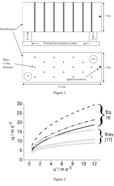
The experimental rig was of steel construction and measured 8.25m in length,

3.0m in width, and 2.8m in height. One 3.02.8m end of the rig was effectively open

retain the gas-air mixture prior to ignition. Figure 1 depicts the rig, and indicates the

configuration of pipe-work congestion and the spark ignition points, although not to

scale.

The gases investigated were mixtures of methane, hydrogen, and air, with the

hydrogen-to-methane ratio by volume being 0:100, 20:80 and 50:50. Methane and

hydrogen were introduced into the enclosure from separate gas supplies and then the

mixture recirculated using an external system containing a fan. A composition with an

equivalence ratio of 1.1 was selected, being that expected to generate the highest

overpressures. Table 1 contains a summary of the test programme and hence the

configurations used in the subsequent mathematical modelling reported in this paper.

The reader is directed to the aforementioned publication [2] for further details

regarding the experiments.

Experiment number

Fuel / CH4:H2

Congestion / number pipes

Ignition location

1 100:0 None Centre

2 80:20 None Centre

3 50:50 None Centre

4 80:20 17 Centre

5 50:50 17 Centre

6 100:0 None Rear

7 80:20 None Rear

8 50:50 None Rear

9 80:20 17 Rear

10 50:50 17 Rear

2.2 Turbulent Flow Calculations

Predictions were based on the solutions of the ensemble-averaged,

density-weighted forms of the transport equations for mass, momentum, total energy, and a

reaction progress variable. The latter two equations are defined in Section 2.3. Closure

of this equation set was achieved via compressibility-corrected forms of the k- [6]

and a Reynolds stress [10] transport turbulence model in an attempt to elucidate their

different qualities in such applications. Solutions to the time-dependent forms of the

descriptive equations were obtained using a modified version of a general-purpose

fluid dynamics code referred to as QICA, and provided by Mantis Numerics Ltd.

Within this code, integration of the equations employed a second-order accurate

finite-volume scheme in which the transport equations were discretised following a

conservative control-volume approach with values of the dependent variables being

stored at the computational cell centres. Approximation of the diffusion and source

terms was undertaken using central differencing, and a second-order accurate variant

of Godunov’s method applied with respect to the convective and pressure fluxes. The

fully-explicit time-accurate method was a predictor-corrector procedure, where the

predictor stage is spatially first-order, and used to provide an intermediate solution at

the half-time between time-steps. This is then subsequently used at the corrector stage

for the calculation of the second-order fluxes. A further explanation of this algorithm

can be found elsewhere [12]. The calculations also employed an adaptive

finite-volume grid algorithm which uses a two- or three-dimensional rectangular mesh with

grid adaption achieved by the successive overlaying of refined layers of

computational mesh. Each layer is generated from its predecessor by doubling the

number of computational cells in each spatial direction. This technique [13] enables

variables, and conversely, relatively coarse grids where the flow field is numerically

smooth. Additionally, the updating of the grids after each time-marching cycle

ensures that the required resolution always follows the movement of flow features

such as the flame front.

2.3 Premixed Combustion Model

The turbulence and premixed combustion interaction was represented using a

method first introduced by Catlin and Lindstedt [8]. This semi-empirical approach

incorporates the effects of kinetic and turbulence influences upon the burning velocity

of the flame whilst also retaining a realistic flame thickness throughout the

computation. Following the method of Catlin et al. [7], this approach was

implemented by the solution of equations representing a reaction progress variable

and the total energy of the mixture, in addition to the equations describing the fluid

flow. The former are defined as:

 

 

 

i i i

c c c

u S c

t  x  x x 

   _  _  _  _{ }      _  _     (1)

 

 

 

 

 

i i i i i

E E p T

u u u C S E

t x x x x x

                _ _       _  _   

   (2)

The reaction progress variable is defined as Equation (3):

,0 1 f f Y c Y     _ _      (3)

and is such that it takes a value of 0 in the unburned mixture and 1 in the burned. The

total energy of the mixture is defined as:

2

1 2 i

E  e u k where

0

T v T

The stress tensor evident in Equation (2) is represented by either a Boussinesq

relationship or by substitution with its transported value, when applied with the

two-equation or Reynolds stress turbulence model, respectively. The source terms in

Equations (1) and (2) are related to a modified form of the eddy break-up reaction rate

expression in the following manner:

 

S c R

  (5)

 

S E R q

  (6)

where





2

4

1 u

c

b

R Rc c 

 



 

 _{  }

 

  (7)

and





q  

  

  

_{ }  _ 

   (8)

In the study of Catlin and Lindstedt [8], the form of the reaction rate term as defined

by Equation (7) was derived so as to eliminate the cold front quenching problem by

prescribing variation of the reaction rate throughout the flame thickness based upon a

power law expression. This removes the requirement to explicitly specify a quench

criterion. Additionally, an eigenvalue analysis of the steady-state flow equations of

one-dimensional planar flames propagating in constant turbulence provided unique,

expansion-ratio independent values for the burning velocity and flame thickness

eigenvalues. Hence, these quantities are expressed as:

 

t

u   R (9)

1 2 2 t R  _{   } 

  (10)

and subsequent formulations of the diffusion coefficients and source terms in

1 2 l t c c u  _        _{ } _{ }    

  (11)

1 2 l t T T u  _        _{ } _{ }  

    (12)

 





S c c c 

          _{    } 

     (13)

where the flame thickness is taken to be a turbulence length scale, given by:

3 2 3 4 t k l C_





  (14)

2.4 Turbulent Burning Velocity

It now only remains to prescribe a value for the turbulent burning velocity of the

mixture to fully close the equation set. This was effected through use of the results of

an analysis [14] of numerous detailed experimental data sets obtained during the

complementary burning velocity studies undertaken at the University of Leeds [3].

The method of applying the newly-derived laminar and turbulent data within the

framework of the fluid dynamics code was then in principle that outlined by Catlin et

al. [7] who alternatively applied expressions describing the turbulent burning velocity

based upon the data of Abdel-Gayed et al. [15] and the formulations of Gulder [16]

and of Bray [17].

The experimental data of Fairweather et al. [3] was made available in a similar

form to that of Bray [17] in that it is presented as a function of the Karlovitz stretch

factor, K. Two correlations are proposed [14] for hydrogen content between 0 and

20%, and for a 50% concentration by volume as:

( 0.49)

0 20% t 0.37

l l

u u

K

u u

 

( 0.47)

50% t 0.54

l l u u K u u    (16) where 2 1 0.157 l l u K u R    _{ }

  (17)

and t

l

l R u 





 (18)

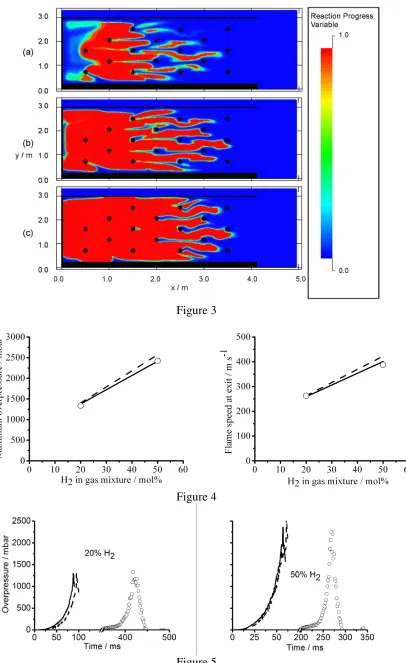
Figure 2 presents a performance comparison of the correlations of Bray [17] and of

and the expressions above at three arbitrary values of the turbulence kinetic energy.

Plotted is the predicted turbulent burning velocity against increasing values of the

r.m.s. of the turbulent fluctuating velocity, and it is evident that the new correlations

do predict magnitudes notably smaller than their predecessors. Although inconclusive

in its own right, these observations are conforming with those made by Catlin et al.

[7] when undertaking similar comparisons of burning velocity correlations.

The remaining unknown in Equations (15), (16), and (17) is the laminar burning

velocity of the fluid which was again prescribed from the experimental observations

of Fairweather et al. [3] and Burluka et al. [18] and given values of 0.49, 0.59, and

0.81 m s-1 for the three cases of 0%, 20%, and 50% hydrogen content by volume.

These values were corrected for the effects of temperature and pressure within the

code via the relation [19]:

1 2 2 ,0 0 0 u l l T u u T         _{   }

3. RESULTS AND DISCUSSION

3.1 Three-dimensional Calculations

For these calculations the geometry modelled was a three-dimensional volume

containing the rig discussed in Section 2.1, and shown schematically in Figure 1.

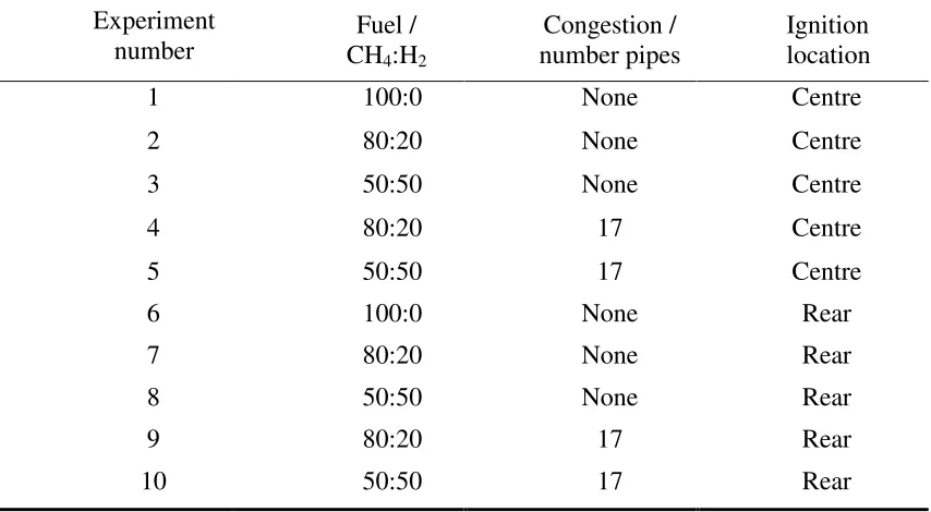
Figure 3 depicts three, two-dimensional planar sections through this geometry, where

the left and upper boundaries represent a solid wall, and the extreme right an outflow

boundary. The lower boundary represents a floor raised slightly above the ground

level of the vessel exterior. The remaining two walls of the vessel were represented as

solid surfaces and hence a complete three-dimensional representation of the vessel

interior was used. These walls are not visible in Figure 3 as they lie on the planes z=0

and z=3. A small area of burned gas, represented by a region where the progress

variable equals 1.0, was initially located adjacent to the left boundary and central to

its face in order to instigate the numerical reaction. The base computational mesh was

dimensioned to be a 2488 grid, with 5 possible levels of grid refinement available.

Sensitivity analyses using varying base meshes and levels of grid refinement indicated

that the results presented below are free of numerical instability and error.

From an assembly of time-lapse sequences of the reaction progress variable such

as those shown in Figure 3, the temporal behaviour of the flame front can be seen to

be in-line with expectation. Initially progressing at a relatively slow rate, the reaction

zone subsequently accelerates through the unreacted fluid upon each obstacle

interaction due to the turbulence induced by flow over the obstacle, returning to a near

constant velocity in between these areas of turbulence generation.

The experimental cases considered using the three-dimensional approach were

those of rear ignition in the congested rigs; namely, experiments 9 and 10 as noted in

computational requirements of the problem dimensionality. One calculation therefore

typically requires 8 gigabytes of volatile RAM and, in the case of geometries with a

large solid/fluid interfacial area, upwards of three weeks to complete using a single

3GHz processor running with a 1.3GHz front side bus. Since completion of this work,

the code has been developed to run on parallel processors, which provides a great

saving on computational time, given suitable available CPU resources.

Analysis of the results provides the maximum overpressures achieved and the

flame front vessel-exit velocities predicted by both the k- and second-moment

turbulence closures, which are presented in Figure 4. It is evident from these results

that the magnitude of the predictions, and hence ultimately their conformity with

experiment, depends upon the turbulence model, which in turn has a performance

dependency upon the fuel being investigated. For the three-dimensional calculations

considered here, the more reliable Reynolds stress model is seen to be at variance with

its two-equation counterpart with respect to recorded maximum overpressures and

exit flame speeds. In these rear ignited cases, and at the high turbulence levels

associated with the congested geometry, the flow becomes increasingly less isotropic

with time and it is likely that a notable component of the turbulence stress-tensor is

not represented accurately in the k- case. Scrutiny of the calculated results also

reveals a relative deterioration of the k- model’s predictive ability in the cases of

higher hydrogen content, this being likely due in part to the introduction of hydrogen

effecting an increase in both the laminar and turbulent burning velocity, and hence an

increase in the turbulence generated. Generally, at the lower hydrogen concentration,

both turbulence models are seen to reproduce experimental evidence well, whereas

the Reynolds stress model appears to be a requisite for more accurate predictions at

Figure 5 shows predicted pressure traces, including peak values, plotted

alongside experimental data for the two cases discussed above. Encouragingly, the

forms of the calculated and experimental traces are very similar. However, there is a

notable discrepancy between the observed times of the calculated and experimental

pressure peaks. A phenomenon observed in reactive systems such as those studied

here is the laminar to turbulent transition behaviour of the proceeding flame front, and

this is notoriously difficult to represent in a mathematical framework. The current

model assumes that the developing flame front initially encounters low levels of

isotropic turbulence to establish a numerically stable solution, and as such no

transitional region is defined. Hence, no distinction is observed between a laminar and

a turbulent development stage numerically. With the rear ignited cases the initial

flame front development occurs in an obstacle-free environment in which the

generation of turbulence energy is minimal. This effects an initially relatively slow

progression of the front through the domain, which reflects the experimentally

observed behaviour of a laminar flame development gradually making a transition to

turbulent. Although the numerical model does not contain a mechanism to account for

the laminar to turbulent transition, when applied to the rear ignited case, the nature of

its obstacle geometry does partly accommodate for this phenomena. This is reflected

in the accurate prediction of peak overpressures, although these do occur far too early

in relation to experimental observation. The experimental data display a region of

laminar growth with respect to overpressure, which then progresses to a period of

rapid accelerating increase, before dropping away with a negative gradient of similar

magnitude. This period of growth delay is not evident in the calculated results,

although the model does reliably predict the rate of significant pressure rise and the

Predicted flame front arrival times obtained using the two turbulence models for

the 20% and 50% H2 cases, corresponding to the results of Figure 5, are plotted

against experimental data in Figure 6. This furthers the previous discussion regarding

the timing of the observed peak overpressures noted in Figure 5, in that although the

calculated rate of significant progress of the reaction front is seen to be in line with

observations, the delay due to the laminar to turbulent transition of the flame is

absent. Figure 6 also confirms the application of the two-equation turbulence model is

predicting generally higher flame velocities than the second-moment closure in these

two cases.

Overall, these three-dimensional calculations yield reasonable predictions of the

propagating turbulent premixed flames of methane and hydrogen which interact with

obstacles within the test vessel considered. In particular, the rate of significant rise in

flame speeds and pressure, and peak overpressures, are in line with experimental

results. In agreement with earlier studies [7, 9], the delay period caused by the

transition of the flame front from laminar to turbulent cannot be accommodated.

However, provided that the high levels of turbulence generated by flow over obstacles

present within the test vessel are predicted accurately, then the significant rise in

flame speed and pressure caused by the flame front interacting with turbulent regions

within the flow are predicted well, and as a result so are the damaging overpressures

that are generated. The present results also show that, although the second-moment

turbulence closure leads to more reliable predictions, the differences between the two

turbulence modelling approaches are not as significant as might be expected.

Additionally, and importantly, these predictions also demonstrate that the turbulent

burning velocity correlations of [3] yield reliable results for the methane-hydrogen

correlations described in Section 2.4, not shown here, which lead to significantly

higher overpressures than observed experimentally due to their over-prediction of the

turbulent burning velocity of methane-hydrogen mixtures, as exemplified by the

results of Figure 2.

3.2 Two-dimensional Calculations

Given the significant computational times required to perform full

three-dimensional calculations, and the inevitable restriction this places on the use of

computational fluid dynamic models in routine consequence and risk assessments, a

second approach of employing a simplified representation of the experiments was also

pursued. In this study, the geometry modelled was a two-dimensional section of that

shown in Figure 1. Figure 7 depicts this geometry and, similarly to the approach used

in modelling the full three-dimensional vessel, the left boundary represents a solid

wall, and the extreme right boundary an outflow. The base and the roof of the vessel

were also represented as solid surfaces, and hence a complete two-dimensional

representation of the vessel interior was used. It was found through trials that an area

external to the vessel also required modelling to ensure representation of the influx of

air from the surroundings into the vessel, and enable meaningful calculations at the

point at which the flame front exited the vessel. Two examples of these calculations

are depicted in Figure 7. The first is the rear ignited case of Experiment 10, and the

second a centrally ignited case, that being Experiment 5. The base computational

mesh was dimensioned to be a 4515 grid, and similarly to the previously discussed

calculations, 5 levels of possible grid refinement were employed. Sensitivity analyses

with differing base meshes and levels of grid refinement again indicated that the

Figure 8 depicts predicted maximum overpressures and vessel exit flame speeds

calculated for all five rear-ignited experimental tests given in Table 1. Similar

observations can be made with respect to the performance of the two different

turbulence models in the case of the vessel containing obstacles as were noted for the

three-dimensional model considered in Section 3.1. However, the varied performance

of the models is highlighted when the results obtained from the calculations of the

empty rig are considered. Here, compared to observations of the relatively high

turbulence cases with obstacles, the Reynolds stress model is seen to predict notably

lower maximum overpressures than its k-counterpart over the three fuels considered.

Generally, the larger discrepancies between the turbulence model predictions and the

data also arise at the higher hydrogen levels, and hence higher flame speeds.

Turning to the predictions of the five centrally ignited cases depicted in Figure

9, results less conforming with experiment are observed in all instances. Maximum

overpressures and exit flame speeds are all seen to be notably over-predicted in all

cases, although the greater accuracy of the Reynolds stress approach is demonstrated

when considering the maximum observed overpressure. For the lower hydrogen

concentration case, its performance is an improvement over the k-approach, and this

is compounded at the 50% hydrogen concentration level. These observed differences

are also reflected in the exit flame speed predictions by an increase in magnitude of

the k-model results over those of the Reynolds stress approach.

The differences in the models’ predictive abilities between the rear- and

centrally-ignited test cases with obstacles warrant further deliberation. As discussed in

Section 3.1, a notoriously difficult to model phenomenon observed in reactive systems

such as those studied here is the laminar to turbulent transitional behaviour of the

represented by an expanding turbulent region located within the matrix of solid

obstacles. With no defined laminar combusting region, interaction between this front

and the obstacles immediately effects the generation of turbulence energy which leads

to the over-prediction of maximum overpressures, with this being increasingly evident

with greater hydrogen concentration. The rear ignited cases do not display a similarly

large over-prediction due to the initial flame front development occurring in an

initially obstacle-free environment in which the generation of turbulence energy is

lower than if centrally ignited.

Analysis of the results pertaining to the non-congested experiments is difficult

due to the evident lack of turbulence and turbulence-generation mechanisms within

the domain. The very nature of the k-and Reynolds stress models makes them suited

to the modelling of regions of high turbulence kinetic energy, or regions with energy

generation mechanisms such as those promoted by the presence of solid obstacles.

The expansion of a progressive flame front through a quiescent volume of gas is not

such an example, and it is hence expected for results to display anomalous qualities

when comparing with the alternate cases. In the rear-ignited 0 obstacle case, it can be

seen that, conversely to the 17 obstacle case, a component of the turbulence is perhaps

not being recorded by the Reynolds stress model. This is to be expected in regions

where turbulence generation is minimal, and the additional energy generated by the

two-equation model is likely to be due to the simplifying assumptions it makes.

Further investigation is warranted to assess the importance of the individual Reynolds

stress components and the applicability of the turbulence modelling approaches for

each experimental condition, although this is difficult in the absence of detailed

Similar statements can be made with consideration of the centrally ignited cases,

in that higher levels of turbulence are generated by application of the two-equation

model, leading to a notable over-prediction of maximum overpressure when compared

to experimental data (Figure 9). The reason for this exaggerated production of

overpressure can be attributed once again to the problem of modelling the laminar to

turbulent transition with such turbulence models. Omitting the effect of such a

transition dictates that the flame kernel growth is influenced by the turbulent burning

velocity at a very early stage, as turbulence kinetic energy is generated with no regard

to laminar development. The assumption of an isotropic eddy viscosity in this instance

is evidently detrimental to prediction, and the Reynolds stress model clearly

demonstrates an improvement over the k- model with prediction of overpressure.

Again, the observable differences between the models become more exaggerated with

increasing hydrogen content, indicating the increase in turbulence energy generation

with increasing reactivity of the fuel.

Drawing comparison with the three-dimensional rear-ignited predictions,

overpressures are seen to be slightly decreased but are of a similar conformity with

experimental data. Exit flame speeds also show a similarity although are slightly

higher than their three-dimensional counterparts. These minor differences are to be

expected due to the three-dimensional model incorporating the physical effects of a

higher-dimensionality. A generally superior performance can be noted in the case of

predictions derived using the second-moment turbulence closure.

Lastly, Figure 10 presents the maximum overpressures observed in calculations

of rear-ignited, 17 obstacle cases using the two-dimensional approach and

k-turbulence model. In addition to the two fuels investigated experimentally, results also

and 50% hydrogen by volume. Evident in this plot is an initial rapid increase in

overpressure with inclusion of 10% hydrogen. Following this, a linear period of

increase is observed between 10 and 45%, at which point an inflection and the

beginning of a likely increased growth phase can be seen. Also shown in this figure

are associated measured and predicted flame speeds at the vessel exit, for which

similar behaviour can be observed. These observations are broadly in line with the

overall findings of the NaturalHy project [1] which established that within buildings,

the severity of explosions is increased if hydrogen is added to natural gas. However,

this increase was judged to be only slight for hydrogen addition up to 20%, with

analysis of experimental and theoretical findings suggesting that the explosion

frequency could increase by a factor of two as a result of adding up to 20% hydrogen

by volume.

4. CONCLUSIONS

For the first time, a Reynolds stress turbulence model has been applied to the

prediction of large-scale vented explosions, coupled to a turbulent premixed

combustion model. Maximum predicted overpressures and flame front velocities for

ten test cases are presented, and comparisons made to calculations based on the k-

model. The Reynolds stress model is seen to generally be at variance with the simpler

turbulence modelling approach, although in terms of predicted overpressures and

flame front velocities these differences are often small. However, the increase in

turbulence anisotropy caused by internal pipe work within a vessel necessitates the

use of a Reynolds stress model on physical grounds alone. These observations are

valid for both approaches used to represent the geometry considered, with the level of

future studies. This study has also demonstrated that the combustion model attributed

to Catlin and Lindstedt [8], incorporated with the most recently available

experimental data collected by Fairweather et al. [3], can model confined, venting

explosions of methane-hydrogen mixtures representing industrial scenarios with a

good degree of accuracy.

It has also been demonstrated that in highly turbulent conditions such as densely

congested regions where the progressing flame front can fully develop within the

domain, both the k- and the Reynolds stress model can accurately model

overpressures and flame speeds in such conditions. However, in conditions such as

those created by the central ignition of the gas volume, or in the uncongested cases

which appear not to permit a full numerical development of the reacting turbulent

medium, the model performance is notably reduced. This is most apparent in the

application of the k- turbulence model, although since both turbulence models

applied assume fully developed turbulent flow their failure to accurately predict the

dynamics of explosions in such situations is to a large extent to be expected.

Although overpressures and flame speeds in the congested cases discussed

previously are modelled well, the arrival times of the flame front throughout the

domains are more difficult to capture. It is concluded that without a mechanism

representing a laminar growth period, followed by the transition to a turbulent flow,

this phenomenon will not be accurately described by the present modelling strategy. It

should however be noted that, as expected, the Reynolds stress model does effect

superior results in the prediction of arrival times over the two-equation approach.

An important observation made during this course of study is that of the

apparent change in gradient of the curve of predicted overpressure at around the 45%

transition to a steeper gradient, which is indicative of a beginning increased growth

phase. This being the case, the 45% level would be a barrier in the consideration of

mixture usage with respect to safety considerations. An increased gradient such as this

is indicative of a rapidly increasing rate of reaction, which in reality may relate to a

5. NOMENCLATURE

c reaction progress variable C_p specific heat at constant pressure

e specific internal energy C_v specific heat at constant volume

k turbulence kinetic energy C_ turbulence viscosity constant

l length scale E total energy

p pressure K Karlovitz stretch factor

t time R reaction rate constant

u velocity S source term

'

u r.m.s. turbulent velocity T temperature

x,y,z spatial coordinates Y mass fraction

Greek Symbols

 ratio of specific heats  density

 flame thickness  Prandtl/Schmidt number

 turbulence kinetic energy  stress tensor

dissipation rate _{c T/} turbulent diffusion coefficient

of c or T

 viscosity  1, 2 eigenvalues

Subscripts

0 initial value j vector indice

b burned l laminar component

f fuel t turbulent component

i vector indice u unburned

6. ACKNOWLEDGEMENTS

The authors wish to thank the European Commission for providing financial support

for this work as part of the Integrated Project NaturalHy (SES6/CT/2004/50266),

funded by the Sixth Framework Programme (2002-2006) for research, technological

development and demonstration (RTD).

7. REFERENCES

[1] NaturalHy, EC funded project, see http://www.naturalhy.net/ (accessed

01/08/12).

[2] Lowesmith BJ, Mumby C, Hankinson G, Puttock JS. Vented confined

explosions involving methane/hydrogen mixtures. Int. J. Hydrogen Energ.

2011; 36: 2337-2343.

[3] Fairweather M, Ormsby MP, Sheppard CGW, Woolley R. Turbulent burning

rates of methane and methane-hydrogen mixtures. Combust. Flame 2009; 156:

780-790.

[4] Bradley D, Haq MZ, Hicks RA, Kitagawa T, Lawes M, Sheppard CGW,

Woolley R. Turbulent burning velocity, burned gas distribution, and associated

flame surface definition. Combust. Flame 2003; 133: 415-430.

[5] Bradley D, Lau AKC, Lawes M. Flame stretch rate as a determinant of

turbulent burning velocity. Phil. Trans. R. Soc. Lond. A 1992; 338: 359-387.

[6] Jones WP, Launder BE. The prediction of laminarization with a two-equation

model of turbulence. Int. J. Heat Mass Tran. 1972; 15: 301-314.

[7] Catlin CA, Fairweather M, Ibrahim SS. Predictions of turbulent, premixed

[8] Catlin CA, Lindstedt RP. Premixed turbulent burning velocities derived from

mixing controlled reaction models with cold front quenching. Combust. Flame

1991; 85: 427-439.

[9] Fairweather M, Hargrave GK, Ibrahim SS, Walker DG. Studies of premixed

flame propagation in explosion tubes. Combust. Flame 1999; 116: 504-518.

[10] Jones WP, Musonge P. Closure of the Reynolds stress and scalar flux

equations. Phys. Fluids 1988; 31: 3589-3604.

[11] Popat NR, Catlin CA, Arntzen BJ, Lindstedt RP, Hjertager BH, Solberg T,

Saeter O, Berg ACVd. Investigations to improve and assess the accuracy of

computational fluid dynamic based explosion models. J. Hazard. Mater. 1996;

45: 1-25.

[12] Falle SAEG. Self-similar jets. Mon. Not. R. Astron. Soc. 1991; 250: 581-596.

[13] Falle SAEG, Giddings JR. Flame capturing. In: Baines MJ, Morton KW,

editors. Numerical Methods for Fluid Dynamics 4, Oxford: Clarendon Press;

1993. p. 337-343.

[14] Fairweather M, Woolley RM, Computational fluid dynamic modelling of gas

explosions in industrial enclosures, EC Naturalhy Project, Work Package 2,

Deliverable D54, Report R0056-WP2-R-0, October 2008.

[15] Abdel-Gayed RG, Bradley D, Lawes M. Turbulent burning velocities: A

general correlation in terms of straining rates. Proc. R. Soc. London A. 1987;

414: 389-413.

[16] Gulder OL. Turbulent premixed flame propagation models for different

combustion regimes. Proc. Combust. Inst. 1991; 23: 743-750.

[17] Bray KNC. Studies of the turbulent burning velocity. Proc. R. Soc. London A.

[18] Burluka AA, Fairweather M, Ormsby MP, Sheppard CGW, Woolley R. The

laminar burning properties of premixed methane-hydrogen flames determined

using a novel analysis method. In: Proceedings of the 3rd European

Combustion Meeting, Chania: Combustion Institute (Greek

Section)/Mediterranean Agronomic Institute of Chania; 2007, Paper 6-4.

[19] Andrews GE, Bradley D. The burning velocity of methane-air mixtures.

FIGURE CAPTIONS

Figure 1 Schematic diagram of the experimental rig.

Figure 2 Comparison of the predictions of two turbulent burning velocity correlations (upper, middle and lower curves correspond to k=5000, 1000 and 500 m2s-2, respectively).

Figure 3 Two-dimensional planar sections of reaction progress variable predictions in the three-dimensional geometry at (a) z=0.15, (b) 0.25, and (c) 1.50.

Figure 4 Maximum overpressures and exit plane flame speeds for the 17 obstacle geometry with rear ignition, and 20% and 50% hydrogen concentrations, calculated using the three-dimensional approach (symbols – experiment; solid line – Reynolds stress; dashed line – k-).

Figure 5 Pressure traces for the 17 obstacle geometry with rear ignition, and 20% and 50% hydrogen concentrations, calculated using the three-dimensional approach (symbols – experiment; solid line Reynolds stress; dashed line – k-)

Figure 6 Flame front arrival times for the 17 obstacle geometry with rear ignition, and 20% and 50% hydrogen concentrations, calculated using the three-dimensional approach (symbols – experiment; solid line Reynolds stress; dashed line – k-).

Figure 7 Plots of reaction progress variable predictions indicating the extent of reaction in rear (upper) and centrally (lower) ignited cases for 50% hydrogen and 17 obstacles calculated using the two-dimensional approach.

Figure 8 Maximum overpressures and exit plane flame speeds for the 0 and 17 obstacle geometries with rear ignition, and 0%, 20% and 50% hydrogen concentrations, calculated using the two-dimensional approach (symbols – experiment: o 17 objects, 0 objects; solid line – Reynolds stress, dashed line – k-).

Figure 9 Maximum overpressures and exit plane flame speeds for the 0 and 17 obstacle geometries with central ignition, and 0%, 20% and 50% hydrogen concentrations, calculated using the two-dimensional approach (symbols – experiment: o 17 objects, 0 objects; solid line – Reynolds stress, dashed line – k-).

Figure 1

Figure 3

Figure 4

Figure 6

Figure 7

Figure 9