Transitions in pathways of human development and carbon emissions

This content has been downloaded from IOPscience. Please scroll down to see the full text.

Download details:

IP Address: 31.185.199.135

This content was downloaded on 26/01/2014 at 21:53

Please note that terms and conditions apply.

Transitions in pathways of human development and carbon emissions

View the table of contents for this issue, or go to the journal homepage for more 2014 Environ. Res. Lett. 9 014011

(http://iopscience.iop.org/1748-9326/9/1/014011)

Environmental Research Letters

Environ. Res. Lett.9(2014) 014011 (10pp) doi:10.1088/1748-9326/9/1/014011

Transitions in pathways of human

development and carbon emissions

W F Lamb

_{, J K Steinberger}

_{, A Bows-Larkin}

_{, G P Peters}

_{, J T Roberts}

and F R Wood

1_{Tyndall Centre for Climate Change Research, School of Mechanical, Aerospace and Civil Engineering,}

The University of Manchester, Room H1, Pariser Building, Manchester, M13 9PL, UK

2_{Sustainability Research Institute and Centre for Climate Change Economics and Policy, School of Earth}

and Environment, University of Leeds, Maths/Earth and Environment Building, Leeds, LS2 9JT, UK 3_{Institute of Social Ecology Vienna, Alpen-Adria University, 29 Schottenfeldgasse, A-1070, Austria}

4_{Center for International Climate and Environmental Research—Oslo (CICERO), PB 1129 Blindern,}

NO-0318 Oslo, Norway

5_{Center for Environmental Studies, Brown University, Box 1943, 135 Angell Street, Providence,}

RI 02912, USA

E-mail:[email protected]

Received 26 June 2013, revised 18 November 2013 Accepted for publication 21 November 2013 Published 15 January 2014

Abstract

Countries are known to follow diverse pathways of life expectancy and carbon emissions, but little is known about factors driving these dynamics. In this letter we estimate the

cross-sectional economic, demographic and geographic drivers of consumption-based carbon emissions. Using clustering techniques, countries are grouped according to their drivers, and analysed with respect to a criteria of one tonne of carbon emissions per capita and a life expectancy over 70 years (Goldemberg’s Corner). Five clusters of countries are identified with distinct drivers and highly differentiated outcomes of life expectancy and carbon emissions. Representatives from four clusters intersect within Goldemberg’s Corner, suggesting diverse combinations of drivers may still lead to sustainable outcomes, presenting many countries with an opportunity to follow a pathway towards low-carbon human development. By contrast, within Goldemberg’s Corner, there are no countries from the core, wealthy consuming nations. These results reaffirm the need to address economic inequalities within international

agreements for climate mitigation, but acknowledge plausible and accessible examples of low-carbon human development for countries that share similar underlying drivers of carbon emissions. In addition, we note differences in drivers between models of territorial and consumption-based carbon emissions, and discuss interesting exceptions to the drivers-based cluster analysis.

Keywords: low-carbon development pathways, sustainable development, climate change, world systems theory

1. Introduction

To avoid ‘dangerous climate change’ it is becoming increas-ingly clear that immediate and sustained reductions in carbon

Content from this work may be used under the terms of theCreative Commons Attribution 3.0 licence. Any further distribution of this work must maintain attribution to the author(s) and the title of the work, journal citation and DOI.

emissions are required by nations (Anderson and Bows2008, Peterset al2011). For developing and transitioning countries, a current challenge is how to mainstream emissions reduc-tions policies within development decisions that potentially ‘lock-in’ patterns of carbon use over decades (Unruh and Carrillo-Hermosilla2006, Halsnæset al2007). While a narrow emphasis on economic growth appears difficult to reconcile

Environ. Res. Lett. (2014) 014011 W F Lambet al

with climate targets (Anderson and Bows2008), a recent focus on non-GDP measures of national progress broadens the scope of measuring real development instead of economic activity (Stiglitz et al 2009, Jackson 2009). An emerging literature in this tradition explores environmental impacts in relation to indicators of human well-being, where countries are shown to perform with varying ‘Ecological Intensities of Well-Being’ (EIWB) (Dietz et al 2007, 2009, 2012, Knight and Rosa

2011, Knightet al2013). Moreover, researchers have found a temporal characteristic to this relationship, revealing diverse country development pathways towards highly differentiated states of carbon emissions and life expectancy (Steinberger and Roberts2010, Steinbergeret al2012). In the absence of a single industrial development trajectory, what are the constraints to pathways of low-carbon human development? This is a subject that will be explored in this letter.

In analysing development pathways, it is of course interesting to understand the underlying drivers of carbon emissions. International diversity makes a driver-based anal-ysis challenging, owing to vast differences in geography and resource endowment, economic status and structure, and the governance or institutional structures that influence national carbon emissions. In addition, development pathways evolve within the world system; they are subject to external influence through international agreements, exchange relations and global flows of carbon emissions embodied in manufactured goods (Roberts and Parks2007,2009, Peters2008). Studies on the drivers of carbon emissions may explore socio-economic factors such as population, affluence and technology, typically formulated through the IPAT or Kaya Identities (Kaya1990, Ehrlich and Holdren1972). These factors can be expanded to include a wider range of variables, including geophysical ones within the more flexible and empirical STIRPAT framework (Yorket al2003a). Whereas the Kaya Identity allocates emis-sions to predefined factors, STIRPAT enables the empirical testing and quantification of the contribution of a diversity of drivers.

To our knowledge, few studies have examined the cross-national distribution of emissions drivers (e.g. Jorgensonet al

2009, Jorgenson and Clark2011,2012, Jorgensonet al2012, Jorgenson and Clark2013). None have focused on the differ-ences between consumption-based and territorial emissions. Ecological Intensity of Well-Being research has also tended to employ the ecological footprint as an indicator of environmen-tal impact (Dietzet al2007,2009,2012). While the ecological footprint allocates externalities to consumption, it has several weaknesses. Among the foremost, the ecological footprint in the standard methodology collapses seemingly incommensu-rate dimensions into one variable, and in employing apparent consumption renders the allocation of emissions arising from the indirect use of goods and services problematic (Wiedmann

2009, Borucke et al 2013). The recently established global database for CO2emissions using a multi-region input–output (MRIO) methodology provides an opportunity to examine the well-being implications of both direct and indirect consump-tion activities (Peterset al2011, Steinbergeret al2012).

In this letter, we seek to identify clusters of countries that share similar underlying drivers of carbon emissions,

to explore opportunities for low-carbon transitions going forward. Our aims are to first identify the cross-sectional drivers of consumption-based emissions (Peterset al2011), and quantify their strength using multiple regression. Second, we perform cluster analysis on significant drivers in the model to group countries and analyse them with respect to a sustainability criteria of low-carbon emissions and high life expectancy. The goal of this driver-based clustering is to understand and analyse countries: not on the basis of their actual emissions, or from the usual simplification of GDP and regional groupings such as Europe, Asia and so on, but from the factors actually driving the emissions. We will thus be able to discuss meaningful differences and similarities in the underlying factors driving emissions, including differences in the resulting emissions, with implications for transformative pathways of low-carbon human development. We begin with a section on materials and methods, followed by results and discussion, and conclusions.

2. Materials and methods

2.1. Data

2.1.1. Dependent variables. In contrast to other studies, we use consumption-based carbon emissions, where emissions equal the domestic use of fossil fuels plus the embodied emissions from imports, minus exports (Peterset al2011). Our analysis of consumption-based estimates are also compared to the more commonly used territorial-based accounts, which capture the emissions from domestic activities only (Boden

et al 2013). Steinberger et al (2010) recently demonstrated a stronger statistical relationship between consumption-based emissions and life expectancy compared to territorial emis-sions, thus our focus remains on the former as it appears to better describe the accrued benefits to human well-being of emissions activities. Both measures of carbon emissions are normalized by population, as per capita (intensive) values allow for comparability between countries of different scales. This process assumes a population coefficient of 1 with total emissions, a standard result of cross-sectional studies (Dietz and Rosa 1997, York et al 2003b, Steinberger et al 2010), but one which may not hold for time-series analysis, where elasticities higher or lower than 1 have been observed (Shi

2003, Wei2011, Jorgenson and Clark2013).

2.1.2. Independent variables. Guided by the discussion in Rosa and Dietz (2012), we consider six drivers of national carbon emissions identified in the literature (table1). These can be broadly categorized as economic (GDP/capita, share of exports in GDP), demographic (population growth, urbanisa-tion) and geographic variables (climate, population density).

Environ. Res. Lett.9(2014) 014011 W F Lambet al

Table 1. Drivers of national carbon emissions.

Variables Unit Year

Economic

Income (GDP/capita) $ (PPP 2005 $ international) 2008

Exports % of GDP 2008

Demographic

Population growth % (5 year growth rate) 2005–2010 Urbanisation % of population in urban areas 2008

Geographic

Climate ◦C (three month winter average temperature) 2002 Population density People/sq. km land area 2008

urbanisation may deliver economies of scale for transportation and household services, resulting lower average emissions (Weisz and Steinberger2010). Geographic endowments may influence emissions through increased heating requirements in colder, temperateclimates(Neumayer2002,2004). Popu-lation densityresults in different expectations of resource use more broadly, as an indicator of agricultural development and resource scarcity (Krausmann et al 2008). In the economic category,incomeis a well understood and powerful driver of national emissions, but does not have an inverted U-shaped relationship from the consumption-based perspective (Envi-ronmental Kuznets Curve) (Rothman 1998, Galeotti et al

2009, see Stern 2004 for a review). For this study we are also interested in the effect of participation in the global economy. Theoretical and empirical research has revealed diverging impacts of trade—improving environmental quality in wealthy Northern countries, and an increasing impact of production activities in the global South (Jorgenson and Clark

2012, Roberts and Parks2007,2009), thus we also include a term fortrade openness(the share of national exports of goods and services in GDP), to explore groups of countries that are economically open or alternatively self-contained.

2.1.3. Sources. The data used was sourced as follows: popu-lation growth and popupopu-lation density from the United Nations Development Program (UNDP2013); urbanisation, GDP (PPP 2005 $ international) and the export share of GDP from the World Bank Development Indicators (World Bank2013); climate data was compiled from three month winter average minimum temperatures (Mitchellet al2002). Consumption-based carbon emissions were sourced from Peterset al(2011), and territorial emissions from Bodenet al(2013). 2008 was the baseline year for reporting (set as the latest year in the dependent variable dataset), however as population growth is reported in 5 year intervals, in this case 2010 was used. We assume that temperature data from 2002 is still representative of the 2008 climate in terms of systematic differences between countries.

The maximum sample size across all variables in the dataset was used, comprising 87 countries. From this, three city states were removed due to their outlier behaviour: Singapore, Hong Kong and Luxembourg6. We acknowledge the relatively

6 _{According to the dataset Luxembourg and Singapore have}

consumption-based carbon emission profiles twice as large as commensurate economies in

small size of this sample, which does not include most small island nations, oil exporters and many low-income countries. This is due to the newness of consumption-based emissions accounting: results may be improved as these datasets develop and diffuse. Nevertheless, 84% of the global population was captured in our study, and of global CO2 emissions in 2008 the 84 countries represented 81% and 82% respectively from consumption-based and territorial perspectives.

2.2. Methods

2.2.1. Multiple regression. Multiple least squares regression is applied initially to six drivers to estimate models of consumption-based and territorial emissions. We use a log form multiplicative model, as is usual in the STIRPAT literature (Dietz and Rosa1994). To address colinearity, we calculated variance inflation factors (VIF) for the independent variables and reviewed correlation coefficients (appendixB). We considered only significant variables for the final cluster analysis (p<0.1), repeating VIF tests for this smaller subset of drivers with consistent inflation factors in the range of 1.1–1.6. As is usual in this type of analysis, we included a quadratic term for income, with results described in appendixA.

2.2.2. Cluster analysis. To group and identify patterns of drivers across the sample of countries, cluster analysis is applied to a final subset of significant drivers derived from the regression model. The clustering methodology was chosen to take account of differences in the units of each variable, and consistency in the size and distribution of resulting clusters. Further information on the choice of algorithm, the standardisation method, and the number of clusters chosen in the final analysis are included in appendixA. It should be noted that the clustering methodology equally weights all variables, therefore the results of this grouping will not reflect the relative strengths of the drivers.

3. Results and discussion

3.1. Drivers of national carbon emissions

The variables showing strongest explanatory power for a model of consumption-based emissions are income, climate,

Europe and East Asia (over 9 tons of carbon per capita); while Hong Kong shifts from under 1 tonne to over 6 tonnes of carbon emissions in a period of just one year.

Environ. Res. Lett. (2014) 014011 W F Lambet al

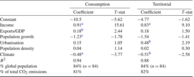
Table 2. Regression models of consumption and territorial-based carbon emissions. (Note: all variables are on a log scale.)

Consumption Territorial

Coefficient T-stat Coefficient T-stat

Constant −10.5 −5.62 −4.77 −1.62

Income 0.91a 15.61 0.83a 9.10

Exports/GDP 0.18b 2.44 0.18 1.50

Population growth −1.23c −1.78 −1.54 −1.41

Urbanisation 0.15 1.05 0.48b 2.19

Population density 0.04 1.14 0.02 0.30

Climate −0.48a −3.77 −0.51b −2.58

R2 0.94 0.88

% global population 84% (n=84) 84% (n=84)

% of total CO2emissions 81% 82%

a_{Indicates statistical significance atp<0.001.} b_{Indicates statistical significance atp<0.05.} c_{Indicates statistical significance atp<0.10.}

exports and population growth (table2). Income has the great-est statistical significance and scales positively with carbon emissions. The climate variable, measuring the coldness of a country’s winter, also has a significant and strong negative coefficient in the model, confirming that warmer countries tend to have lower levels of carbon emissions where other factors are held constant. The openness of an economy, its export share of GDP, shows a positive relationship with levels of consumption emissions. Unlike York (2007), we find a negative effect of population growth on carbon emissions. In addition, we find no relationship between population den-sity and urbanisation with increased carbon emissions. The goodness of fit (adjustedR2) for a model combining income, exports, population growth and climate is 0.94; a high level of explanatory power, but nonetheless within the range of similar studies (Liddle and Lung2010, Steinbergeret al 2012), and expected due to the level of correlation between income and carbon emissions (appendix B). Based on a criteria of p<

0.1, four variables—income, exports, population growth, and climate—are suitable for the drivers-based cluster analysis.

The shift from territorial to consumption-based emissions inventories implies a corresponding change in the underly-ing drivers of those emissions. As noted in previous work, this shift tends to increase carbon responsibility in wealthy consuming nations while decreasing responsibility in less wealthy producing nations (Peterset al2011, Steinbergeret al

2012). Thus it is no surprise that income is a highly dominant predictor of emissions in our regression model. Similarly, we might expect the global trade in emissions to lessen the impact of domestic characteristics on patterns of consump-tion, in favour of economic status. Comparisons between two models of consumption and territorial emissions support this view: statistical significance declines for urbanisation in the consumption-based model, and increases markedly for income and exports (table2). The dependence of consumption-based emissions on the export share of GDP might be seen as redundant, since consumption-based emissions remove ex-ports and add imex-ports to territorial emissions. However, it is notable that the correlation is positive, indicating that trade

openness is the main driver, rather than traded emissions. The importance of urbanisation for territorial emissions requires its own explanation: urban areas are generally more affluent and connected to energy networks, ceteris paribus: but in a consumption perspective, income and trade come to dominate, and urbanisation diminishes as an explanatory factor.

The final variables in the analysis are notably related to the development status of nations. Population growth is a factor in the global demographic transition, a co-evolution of rising incomes with slowing population growth, increasing median age and the shift of households from rural to urban areas (Kirk 1996). Trade openness as a key driver of economic growth is at the centre of empirical and theoretical debates between the structuralist and neoliberal schools of develop-ment theory (Gwynne and Kay 2000). In addition, climate has been extensively studied as a driver of development, through channels of agricultural performance and morbidity (Diamond1997), and more convincingly as a proxy for the colonial origins of comparative development (Acemogluet al

2002). More practically, cold climates drive emissions use for heating applications (York et al 2003a, 2003b, Dietz et al

2007, Steinbergeret al2010), which is likely to be the effect we observe in our analysis, since economic development is already well represented through other variables. We can understand the negative effect of population growth on per capita emissions through other demographic effects, such as larger household sizes (leading to economies of scale), and a higher proportion of children (and resulting lower emissions per capita). How are these factors distributed across countries? We turn to this question in section3.2.

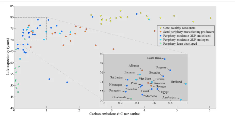
3.2. Grouping countries with similar drivers

Environ. Res. Lett.9(2014) 014011 W F Lambet al

where the five clusters of countries are differentiated by colour. Just as a reminder: neither emissions nor life expectancy are used as variables in the cluster analysis. We expect to see results broadly reflecting the global economic hierarchy, but with some interesting exceptions.

The clusters are in part characterized by terms common in the world systems theory literature (Van Hamme and Pion

2012, Robertset al2003): ‘core’ advanced countries of the world system, which are predominantly supplied through trade by a ‘semi-periphery’ of aspiring nations, and a more distant ‘periphery’ of least developed nations (table3). Thus the first group, the ‘Core: wealthy consumers’ contains the developed economies of Europe, North America and East Asia. This cluster experiences cold winters, has very low population growth rates and an average 47% share of exports in GDP. The core countries occupy a position of very high life expectancy, with none below 75 years (figure1), yet range in carbon emissions from 2.5 tonnes per capita to over 6 tonnes. A second group of countries, the ‘Semi periphery: transitioning producers’, comprises the majority of former communist states, as well as China and central Asia. These countries have medium incomes, on average negative rates of population growth and experience very cold winters. On average, 48% of their economies are based on trade. In part due to political upheaval after the collapse of the former Soviet Union, the opportunity for human development has been stunted in the transitioning producers. They occupy a lower range of life expectancies from 67 to 77 years of age, again with a broad spread of carbon emissions from 0.5 to 4.2 tonnes per capita.

The ‘Periphery 1: moderate income and closed’ is a large cluster of poor to middle income economies, comprising a diverse mix of countries in South and East Asia, Central and South America, and North Africa. This group has typically warm winters, a moderate population growth rate averaging 1.3% and a relatively small share of exports at 31%. On first glance this cluster is perhaps the least well defined in terms of its human development outcomes and levels of national carbon emissions, but in both measures we can recognize outliers of extremely low life expectancies (South Africa and Botswana, countries suffering from an AIDs epidemic) and very high-carbon emissions (New Zealand and Australia, which have ‘attached’ to this cluster due to warmer winters, high population growth rates and strong export structures based on natural resources). Where these countries are discounted, life expectancies range from just under 65 years to as high as 78 years, with a tight spread of emissions between 0.1 and 1.5 tonnes of carbon per capita. A similar cluster, ‘Periphery 2: moderate income and open’, is differentiated from this group by its extremely high average export percentage of GDP (75%). This is a small cluster, made up of mainly South-East Asian states7that achieve life expectancies between 62 and 76 years, and emissions ranging from 0.4 to 1.8 tonnes per capita. Finally, the ‘Periphery 3:

7 _{One outlier from the developed region, the small island EU nation Malta,}

is also present in this group with carbon emissions of 4.1 tons per capita and 79 years of life expectancy. It has been clustered with the ‘Periphery: moderate income and open’ due to its extremely high export percentage of GDP.

least developed’ countries are made up of predominantly African nations. They are very poor, participate very little in global trade, have high population growth rates and very warm climates. This cluster has the highest range of life expectancies, from just 47 years to 71; none have carbon emissions greater than 0.3 tonnes per capita.

The boxed area indicates a region of particular interest: carbon emissions lower than 1 tonne per capita and life expectancies greater than 70 years, ‘Goldemberg’s Corner’ (Steinberger and Roberts 2010). Countries within Goldem-berg’s Corner are able to balance both high human develop-ment and low-carbon emissions, meeting two basic dimen-sions of sustainability critical for climate change mitigation. Four clusters countries intersect here: Albania, Armenia and Georgia from the ‘Semi-periphery: transitioning producers’, as well many countries from ‘moderate income and open’, ‘moderate income and closed’ periphery 1 and 2 groups, and Guatemala from the ‘Periphery 3: least developed’ cluster. This is an important finding, since it indicates that countries with a great variety of underlying drivers can achieve high life expectancies and low emissions. Combinations of hot or cold winters, openness to trade, or not, and high or low rates of population growth can lead to sustainable outcomes—so long as they remain within the constraints of low to medium incomes. The inset of Goldemberg’s Corner in figure1shows a similar diversity in geographic origin. Many countries are Central and South America, but there are also representatives from South-East Asia, Europe and North Africa.

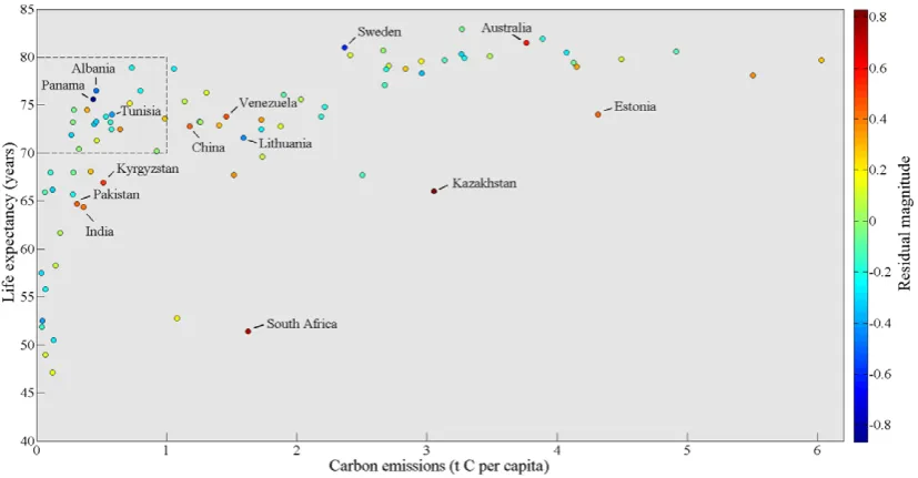
An obvious question to answer is whether these ‘Goldem-berg Corner’ countries are adequately or accurately modelled by the drivers of carbon emissions. FigureB.1in appendixB

represents how well countries fit the regression model by plotting residuals for each country on a colour scale, with those that are particularly poorly modelled (r= >0.4|< −0.4) labelled in text. Within Goldemberg’s Corner, three countries appear to be far more efficient in their national carbon emissions given the structure of independent variables in the model: Albania, Panama and Tunisia. Outside this area Sweden, Lithuania and Uganda are also performing better than expected. Lower performance can be observed in several emerging states (China, India, Pakistan, South Africa), central Asian countries (Kyrgyzstan and Kazakhstan), Australia, Esto-nia and Venezuela. Encouragingly there are no general trends of high magnitude residuals: neither the individual clusters, nor the region of high performing countries within Goldemberg’s Corner as a whole are poorly explained by the model.

High residuals for individual countries are perhaps ex-plained by ‘missing’ drivers in the model. Sweden, for in-stance, is the country within ‘Core: wealthy consumers’ with the lowest carbon emissions. In this case, the absence of a variable representing access to renewable forms of energy generation within the model may explain its exceptional posi-tion (Burke2010,2012). Another illustrative case is Panama, a country with a particularly high export share of GDP. Panama’s lower than expected emissions are likely due to its unique geographic position as an international shipping route, gen-erating a large ‘export’ revenue, while insulating it from climate responsibility under a consumption-based accounting

Environ. Res. Lett. (2014) 014011 W F Lambet al

Figure 1. Simultaneous visualisation of drivers-based clusters (colour legend), life expectancy and carbon emissions. The inset area shows

countries in ‘Goldemberg’s Corner’, a region of less than 1 ton of carbon emissions per capita and greater than 70 years of life expectancy.

Table 3. Means (and standard deviations) for each cluster.

Core: wealthy consumers

Semi-periphery: transitioning producers

Periphery 1: moderate income and closed

Periphery 2: moderate income and open

Periphery 3: least developed

Income per capita ($) 32 955 (7020) 11 620 (5656) 8725 (7300) 9307 (6081) 1442 (1093)

Exports/GDP (%) 47 (20) 48 (19) 31 (10) 74 (15) 28 (8)

Population growth (%) 0.64 (0.42) −0.04 (0.54) 1.30 (0.37) 1.09 (0.45) 2.69 (0.32)

Climate (◦C) −5 (8) −10 (7) 14 (7) 14 (9) 17 (3)

approach. Further disaggregated variables of trade structure may reveal interesting dynamics in this respect. Conversely, China, India, and South Africa are notable countries with higher than modelled emissions. A plausible missing driver for these countries is significant coal deposits, which form the basis of a large portion of their installed electricity generation capacity. Carbon exporters are also known to under-perform in economic terms, even when trade is accounted for Steinberger

et al(2012). These examples embody national endowments of limited comparative value to other nations seeking low-carbon transitions. But despite this, the remaining countries within Goldemberg’s Corner are well explained by the drivers. In fact, the country with the greatest development outcomes under one tonne of carbon emissions per capita, Costa Rica, has a marginal residual, offering an accessible example of national progress to others within its cluster.

4. Conclusions

The acknowledged interactions between drivers of carbon emissions and economic development generate clusters clearly reflecting the international hierarchy of development. Horn-borg (2009) conceives these differences between groups of

countries not as development stages in historical time, but ‘inequalities in societal space’. In addition to economic in-equalities, one might argue for favourable geographies, social conditions or trade interactions in allowing a select group of countries to achieve low-carbon pathways. Yet encour-agingly, our analysis highlights examples from across four clusters of countries that have demonstrated outcomes of high life expectancies and low-carbon emissions. Thus transitions should not seek necessarily to emulate specific high performers such as Costa Rica, or world average performance (Costa

et al2011), these being largely inaccessible and of unclear significance to most countries; rather they may take account of the diverse conditions under which many nations within Goldemberg’s Corner have already achieved pathways of sus-tainable development.

Environ. Res. Lett.9(2014) 014011 W F Lambet al

within Goldemberg’s Corner (notably former Soviet countries, and to a lesser degree northern African nations), it may be interesting to separate out the effects of this apparently important driver of emissions in order to seek mitigation options that are available to all nations; certainly this type of analysis may build upon efficiency frontier methods explored by Dietzet al (2009). Whether these options can result in a global cumulative emissions budget appropriate with current aspirations for ‘safe’ levels of climate change is also a key concern. Finally, the consistent presence of South and Central American economies within Goldemberg’s Corner raises in-teresting questions about the conditions, both nationally and within the world system, cultivating the emergence of this new class of ‘sustainable states’ that are already leading the transition to a low-carbon future.

Acknowledgment

With thanks to Alys Kay and the Graduate Development Office at the University of Manchester.

Appendix A. Methods

A.1. Regression

It is a common procedure in the literature to test for the proposed non-linear effects of affluence on carbon emissions described by the ‘Environmental Kuznets Curve’ (EKC). As we employ consumption-based emissions in our analysis, unlike territorial emissions we do not expect to observe a down-turn for countries in the later stages of development (Rothman

Table A.1. Regression models of consumption and territorial-based carbon emissions. (Note: all variables are on a log scale.)

Consumption Territorial Coefficient T-stat Coefficient T-stat

Constant −14.98 −4.08 −25.20 −4.85

Income per capita 1.74a 2.93 4.65b 5.52

Exports/GDP 0.17c 2.28 0.12 1.14

Population growth −0.74 −0.96 0.70 0.64

Urbanisation 0.07 0.46 0.13 0.61

Population density 0.04 1.24 0.03 0.64

Climate −0.53b −4.04 −0.74b −4.03

Income per capita (quadratic) −0.05 −1.42 −0.21b −4.56

R2 0.94 0.88

% global population 84% (n=84) 84% (n=84)

% of total emissions 81% 82%

a_{Indicates statistical significance atp<0.01.} b_{Indicates statistical significance atp<0.001.} c_{Indicates statistical significance atp<0.05.}

Figure B.1. Simultaneous visualisation of drivers-based model residuals (colour scale), life expectancy and carbon emissions.

Environ. Res. Lett. (2014) 014011 W F Lambet al

1998). This assumption is born out where a quadratic term for income is included in the regression model (tableA.1).

A.2. Cluster analysis

The clusters were generated using a k-means algorithm, in the following process: (1) Random starting positions in the dataset (‘means’) are generated for a predefined number of clusters (2). Observations are associated with their closest mean (3). The geometric centre of each cluster forms a new mean (4). Steps (2) and (3) are repeated until sum of squares within each cluster is minimized. We tested bothk -means and hierarchical clustering using average, single, ward

and weighted aggregation methods. K-means was found to demonstrate consistent results with clusters of appropriate size. All variables were transformed to Euclidean distances (given a mean of zero and standard deviation one) to standardise their different units. An important step in cluster analysis is choosing the appropriate number of clusters. Our procedure was to observe the centroid positions for each new cluster, and determine the dimensions of new variance explained by additional cluster. We rejected a sixth cluster, which generated a new group from a marginal difference in one variable.

Appendix B. Additional tables and figures

Figure B.2. QQ plot of independent variables, indicating the normal distribution of regression residuals.

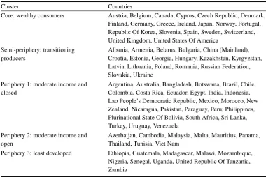
Table B.1. List of countries in each cluster.

Cluster Countries

Core: wealthy consumers Austria, Belgium, Canada, Cyprus, Czech Republic, Denmark, Finland, Germany, Greece, Ireland, Japan, Norway, Portugal, Republic Of Korea, Slovenia, Spain, Sweden, Switzerland, United Kingdom, United States Of America

Semi-periphery: transitioning producers

Albania, Armenia, Belarus, Bulgaria, China (Mainland), Croatia, Estonia, Georgia, Hungary, Kazakhstan, Kyrgyzstan, Latvia, Lithuania, Poland, Romania, Russian Federation, Slovakia, Ukraine

Periphery 1: moderate income and closed

Argentina, Australia, Bangladesh, Botswana, Brazil, Chile, Colombia, Costa Rica, Ecuador, Egypt, India, Indonesia, Lao People’s Democratic Republic, Mexico, Morocco, New Zealand, Nicaragua, Pakistan, Paraguay, Peru, Philippines, Plurinational State Of Bolivia, South Africa, Sri Lanka, Turkey, Uruguay, Venezuela

Periphery 2: moderate income and open

Azerbaijan, Cambodia, Malaysia, Malta, Mauritius, Panama, Thailand, Tunisia, Viet Nam

Environ. Res. Lett.9(2014) 014011 W F Lambet al

Table B.2. Coefficients of correlation.

Carbon emissions (consumption) Carbon emissions (territorial) GDP per capita Exports/ GDP Population growth Urbanisation Population density Climate Carbon emissions (consumption) Carbon emissions (territorial) 0.885

GDP per capita 0.911 0.78

Exports/GDP 0.328 0.221 0.235 Population

growth

−0.447 −0.41 −0.386 −0.273

Urbanisation 0.627 0.59 0.654 0.158 −0.463 Population

density

0.119 −0.059 0.017 0.153 −0.099 −0.05

Climate −0.561 −0.558 −0.482 −0.155 0.633 −0.31 0.09

References

Acemoglu D, Johnson S and Robinson J A 2002 Reversal of fortune: geography and institutions in the making of the modern world income distributionQ. J. Econ.1171231–94

Anderson K and Bows A 2008 Reframing the climate change challenge in light of post-2000 emission trendsPhil. Trans.A

3663863–82

Anderson K and Bows A 2011 Beyond ‘dangerous’ climate change: emission scenarios for a new worldPhil. Trans.A36920–44 Boden T A, Marland G and Andres R J 2013Global, Regional, and

National Fossil-Fuel CO2Emissions(Oak Ridge National Laboratory: Carbon Dioxide Information Analysis Center) Borucke M, Moore D, Cranston G, Gracey K, Iha K, Larson J,

Lazarus E, Morales J C, Wackernagel M and Galli A 2013 Accounting for demand and supply of the biosphere’s regenerative capacity: The National Footprint Accounts’ underlying methodology and frameworkEcol. Indic.24518–33 Burke P J 2010 Income, resources, and electricity mixEnergy Econ.

32616–26

Burke P J 2012 Climbing the electricity ladder generates carbon Kuznets curve downturns∗Aust. J. Agric. Resource Econ.56

260–79

Costa L, Rybski D and Kropp J 2011 A human development framework for CO2reductionsPloS One6e29262 Diamond J 1997Guns, Germs and Steel: The Fate of Human

Societies(New York: Norton)

Dietz T and Rosa E A 1994 Rethinking the environmental impacts of population, affluence and technologyHuman Ecol. Rev.1

277–300

Dietz T and Rosa E A 1997 Effects of population and affluence on CO2emissionsProc. Natl Acad. Sci. USA94175–9

Dietz T, Rosa E A and York R 2007 Driving the human ecological footprintFront. Ecol. Environ.513–8

Dietz T, Rosa E A and York R 2009 Environmentally efficient well-being: rethinking sustainability as the relationship between human well-being and environmental impactsHum. Ecol. Rev.16

114–23

Dietz T, Rosa E A and York R 2012 Environmentally efficient well-being: is there a Kuznets curve?Appl. Geogr.3221–8 Ehrlich P R and Holdren J 1972 A bulletin dialogue on the Closing

Circle. Critique: one-dimensional ecologySci. Public Aff.-Bull. At. Sci.2816–27

Galeotti M, Manera M and Lanza A 2009 On the robustness of robustness checks of the environmental Kuznets curve hypothesis

Environ. Resour. Econ.42551–74

Gwynne R N and Kay C 2000 Views from the periphery: futures of neoliberalism in Latin AmericaThird World Q.21141–56 Halsnæs Ket al2007 Framing issuesClimate Change 2007:

Mitigation. Contribution of Working Group III to the Fourth Assessment Report of the Intergovernmental Panel on Climate Changeed B Metz, O R Davidson, P R Bosch, L R Dave and A Meyer (Cambridge: Cambridge University Press)

Hornborg A 2009 Zero-sum world: challenges in conceptualizing environmental load displacement and ecologically unequal exchange in the world-systemInt. J. Comp. Sociol.50237–62 Jackson T 2009Prosperity Without Growth: Economics for A Finite

Planet(London: Earthscan)

Jorgenson A K and Clark B 2011 Societies consuming nature: a panel study of the ecological footprints of nations, 1960–2003

Soc. Sci. Res.40226–44

Jorgenson A K and Clark B 2012 Are the economy and the environment decoupling? A comparative international study, 1960–2005Am. J. Sociol.1181–44

Jorgenson A K and Clark B 2013 The relationship between national-level carbon dioxide emissions and population size: an assessment of regional and temporal variation, 1960–2005

PloS One8e57107

Jorgenson A K, Clark B and Carolina N 2009 The economy, military, and ecologically unequal exchange relationships in comparative perspective: a panel study of the ecological footprints of nations, 1975–2000Soc. Probl.56621–46 Jorgenson A K, Clark B and Giedraitis V R 2012 The temporal

(In)stability of the carbon dioxide emissions/economic

development relationship in central and eastern European nations

Soc. Nat. Resour.251182–92

Kaya Y 1990Impact of Carbon Dioxide Emission Control on GNP Growth: Interpretation of Proposed Scenarios(Paris: IPCC Energy and Industry Subgroup, Response Strategies Working Group)

Kirk D 1996 Demographic transition theoryPopul. Stud.50361–87 Knight K W and Rosa E A 2011 The environmental efficiency of

well-being: a cross-national analysisSoc. Sci. Res.40931–49 Knight K W, Rosa E A and Schor J B 2013 Could working less

reduce pressures on the environment? A cross-national panel

Environ. Res. Lett. (2014) 014011 W F Lambet al

analysis of OECD countries, 1970–2007Glob. Environ. Change 23691–700

Krausmann F, Fischer-Kowalski M, Schandl H and Eisenmenger N 2008 The global sociometabolic transitionJ. Ind. Ecol.12637–56 Liddle B and Lung S 2010 Age-structure, urbanization, and climate

change in developed countries: revisiting STIRPAT for

disaggregated population and consumption-related environmental impactsPopul. Environ.31317–43

Mitchell T D, Hume M and New M 2002 Climate data for political areasArea34109–12

Neumayer E 2002 Can natural factors explain any cross-country differences in carbon dioxide emissions?Energy Policy307–12 Neumayer E 2004 National carbon dioxide emissions: geography

mattersArea3633–40

Peters G P 2008 From production-based to consumption-based national emission inventoriesEcol. Econ.6513–23

Peters G P, Minx J C, Weber C L and Edenhofer O 2011 Growth in emission transfers via international trade from 1990 to 2008

Proc. Natl Acad. Sci. USA1088903–8

Peters G P, Marland G, Le Qu´er´e C, Boden T, Canadell J G and Raupach M R 2012 Rapid growth in CO2emissions after the 2008–2009 global financial crisisNat. Clim. Chang.22–4 Roberts J T, Grimes P E and Manale J L 2003 Social roots of global

environmental change: a world-systems analysis of carbon dioxide emissions∗J. World-Syst. Res.9277–315 Roberts J T and Parks B 2007A Climate of Injustice: Global

Inequality, North-South Politics, and Climate Policy(London: MIT Press)

Roberts J T and Parks B 2009 Ecologically unequal exchange, ecological debt, and climate justice: the history and implications of three related ideas for a new social movementInt. J. Comp. Sociol.50385–409

Rosa E A and Dietz T 2012 Human drivers of national greenhouse-gas emissionsNature Clim. Change2581–6 Rothman D S 1998 Environmental Kuznets curves—real progress or

passing the buck? A case for consumption-based approaches

Ecol. Econ.25177–94

Shi A 2003 The impact of population pressure on global carbon dioxide emissions, 1975–1996: evidence from pooled cross-country dataEcol. Econ.4429–42

Steinberger J K, Krausmann F and Eisenmenger N 2010 Global patterns of materials use: a socioeconomic and geophysical analysisEcol. Econ.691148–58

Steinberger J K and Roberts J T 2010 From constraint to sufficiency: the decoupling of energy and carbon from human needs, 1975–2005Ecol. Econ.70425–33

Steinberger J K, Timmons Roberts J, Peters G P and

Baiocchi G 2012 Pathways of human development and carbon emissions embodied in tradeNature Clim. Change281–5 Stern D I 2004 The rise and fall of the environmental kuznets curve

World Dev.321419–39

Stiglitz J E, Sen A and Fitoussi J-P 2009Report by the Commission on the Measurement of Economic Performance and Social Progress(Paris: Commission on the Measurement of Economic Performance and Social Progress)

UNDP 2013 Human Development IndicatorsUnited Nations Development Programonline:http://hdr.undp.org/en/statistics/ Unruh G C and Carrillo-Hermosilla J 2006 Globalizing carbon

lock-inEnergy Policy341185–97

Van Hamme G and Pion G 2012 The relevance of the world-system approach in the era of globalization of economic flows and networksGeografiska Annaler: SeriesB9465–82

Wei T 2011 What STIRPAT tells about effects of population and affluence on the environment?Ecol. Econ.7270–4

Weisz H and Steinberger J K 2010 Reducing energy and material flows in citiesCurr. Opin. Environ. Sustain.2185–92

Wiedmann T 2009 A first empirical comparison of energy footprints embodied in trade—MRIO versus PLUMEcol. Econ.68

1975–90

World Bank 2013World Bank Development Indicatorsonline:http: //data.worldbank.org/

York R 2007 Demographic trends and energy consumption in European Union Nations, 1960–2025Soc. Sci. Res.36855–72 York R 2012 Asymmetric effects of economic growth and decline

on CO2emissionsNature Clim. Change2762–4

York R, Rosa E and Dietz T 2003a STIRPAT, IPAT and ImPACT: analytic tools for unpacking the driving forces of environmental impactsEcol. Econ.46351–65

York R, Rosa E and Dietz T 2003b Footprints on the earth: the environmental consequences of modernityAm. Sociol. Rev.68