environments
.
White Rose Research Online URL for this paper:
http://eprints.whiterose.ac.uk/76913/
Monograph:
Salomon, S., Avigad, G., Fleming, P.J. et al. (1 more author) (2013) Active robust
optimization - enhancing robustness to uncertain environments. Research Report. ACSE
Research Reports . Department of Automatic Control and Systems Engineering, University
of Sheffield
[email protected] https://eprints.whiterose.ac.uk/ Reuse
Unless indicated otherwise, fulltext items are protected by copyright with all rights reserved. The copyright exception in section 29 of the Copyright, Designs and Patents Act 1988 allows the making of a single copy solely for the purpose of non-commercial research or private study within the limits of fair dealing. The publisher or other rights-holder may allow further reproduction and re-use of this version - refer to the White Rose Research Online record for this item. Where records identify the publisher as the copyright holder, users can verify any specific terms of use on the publisher’s website.
Takedown
If you consider content in White Rose Research Online to be in breach of UK law, please notify us by
Active Robust Optimization
–
Enhancing
Robustness to Uncertain Environments
Shaul Salomon, Gideon Avigad, Peter J. Fleming, and Robin C. Purshouse
Email:
[email protected]
Research Report No. 1040
Department of Automatic Control and Systems Engineering
The University of Sheffield
Mappin Street, Sheffield,
S1 3JD, UK
Active Robust Optimization – Enhancing
Robustness to Uncertain Environments
Shaul Salomon, Gideon Avigad, Peter J. Fleming, and Robin C. Purshouse
Abstract—Many real world optimization problems involve un-certainties. A solution for such a problem is expected to be robust to these uncertainties. Commonly, robustness is attained by choosing the solution’s parameters such that the solution’s performance is less influenced by negative effects of the un-certain parameters’ variations. This robustness may be viewed as a passive robustness, because once the solution’s parameters are chosen, the robustness is inherent in the solution and no further action, to suppress the effect of uncertainties, is expected. However, it is acknowledged that enhanced robustness comes on the expense of peak performances. In this study, Active Robust Optimizationis presented as a new robust optimization approach. It considers products that are able to adapt to environmental changes. The enhanced robustness of these solutions is attained by adaptation, which reduces the loss in performance due to environmental changes. A new optimization problem named
Active Robust Optimization Problem is formulated. The problem amalgamates robust optimization with dynamic optimization in order to evaluate the performance of a candidate solution, while considering possible environmental conditions. Adaptation’s influ-ence on the solution’s performance and cost is considered as well. Hence, the problem is formulated as a multiobjective problem that simultaneously aims at low costs and high performance. Since these goals are commonly in conflict: the solution is a set of optimal adaptive solutions. An evolutionary algorithm is proposed in order to evolve this set. An example of optimizing an adaptive optical table is provided. It is shown that an adaptive product, which is an outcome of the suggested approach, may be superior to an equivalent product that is not adaptive.
Keywords—robust optimization, dynamic optimization, evolution-ary algorithms, adaptive design, multi-objective optimization.
I. INTRODUCTION
M
OST real world optimization problems involveun-certainties. These uncertainties might be an outcome of, e.g., manufacturing tolerances on components or uncon-trolled changes in environmental conditions. In such cases, the motivation is to identify a solution that is not just an optimal one, but also robust to the uncertainties involved. This kind of optimization is known as Robust Optimization
This research was supported by a Marie Curie International Research Staff Exchange Scheme Fellowship within the7th
European Community Frame-work Programme. The first author acknowledges support from Ort Braude College of Engineering, Israel. The first and second authors acknowledge the hospitality and support of the Mechanical and Material Engineering Department at the University of Western Ontario, Canada.
S. Salomon, P. J. Fleming, and R. C. Purshouse are with the Department of Automatic Control & Systems Engineering, University of Sheffield, Mappin Street, Sheffield, S1 3JD, UK. E-mail: [email protected].
G. Avigad is with the Department of Mechanical Engineering, ORT Braude College of Engineering, 51 Snunit Street, Karmiel, 21982, Israel.
(RO). Some common approaches for RO, such as presented in [1] consider the solution’s expected (mean) performance, its variance or worst case. To ensure robustness, a solution may include some properties that reduce the possible negative influences caused by uncontrolled parameters’ variations (e.g., thick insulation may reduce fluctuations of an oven internal temperature, caused by changes in the ambient temperature).
Many products have some parameters that can be altered while in use. These changes may influence the performances of the product. A tyre’s air pressure, a power drill’s speed, and a cellphone’s screen brightness are examples for such parameters. Adjusting these parameters to account for the effects of uncertainties may improve a product’s performance. If the influence of these adjustable variables is considered during the design phase, the outcome might be a product that is more robust, meaning that its performance is less sensitive to the uncertainties involved.
This conviction may be explained by the cellphone screen example. Suppose that the brightness of a cellphone’s screen is determined by optimizing its battery-life, subjected to sat-isfying the constraint that the screen should be bright enough to enable visibility of the displayed data. The lower the screen brightness, the longer the battery-life and therefore, the lowest brightness that allows visibility should be chosen as the opti-mal value. Since visibility depends on the surrounding light, which is uncertain, RO should be considered. The conventional RO approach will result in a fixed brightness that provides some defined trade-off between optimality and robustness, i.e., the minimal brightness that satisfies the robustness criterion (e.g., based on worst case, mean value, etc.). Such brightness enables visibility in any lighting that is not stronger than a certain level (e.g., daylight with no direct sunlight on the screen). Whenever the surrounding light is weaker than the level considered (e.g., during the night), energy is wasted as the screen is brighter than required. It is clear then, that the phone’s robustness comes at the expense of a shorter battery-life. Moreover, whenever the surrounding light is stronger than the considered level, the data is not visible, and the constraint is violated.
may result in better performance than the conventional RO approach that promotes passive robustness. It is conceivable though that implementing the adjustment might increase the product’s cost.
The process of adjustment to a new configuration as a result of an environmental change is termed here as adaptation. The meanings of other terms that relate to adaptation are as follows: adaptive describes a design or a product that can perform adaptation, and the adaptability of a design defines what properties it can adjust as well as their limits.
This paper introduces a new optimization problem that aims at optimal adaptive products that will promote robustness. The problem, Active Robust Optimization Problem (AROP), considers the influence of the solution’s adaptability both on its performances and its cost. Therefore, it is amulti-objective optimization problem (MOP), and its solution is expected to be a set of optimal adaptive solutions with a trade-off between cost and performance.
The reminder of this paper is organized as follows: In Section II, the position of the current study with respect to the current state of the art in RO is explained, and common definitions of robust and dynamic optimization problems are provided. The AROP is defined and explained in Section III. In Section IV the problem is demonstrated with an example of an optical table design. Finally, conclusions and future research directions are discussed in Section V.
II. BACKGROUND
In this section the required background for understanding the active robustness approach is provided. The terms Dynamic Optimization and Robust Optimization that are the building blocks of the AROP are explained. Existing design and opti-mization methodologies that relate to the AROP are surveyed, and the newly suggested approach is positioned with respect to them.
Robust performance design tries to ensure that performance requirements are met and constraints are not violated due to systems uncertainties and variations. Fundamentally, robust optimization is concerned with minimizing the effect of such variations without eliminating the source of the uncertainty or variation [2]. To search for robust solutions, the variables are treated as stochastic rather than deterministic, while infor-mation about their probability distribution functions (PDF) is taken into account.
There are several approaches for robust optimization. The most common are to represent the performance of a solution by either its expected value [1], or by the worst case (e.g., [3]). If we assume a minimization problem (without loss of generality) then the aim is to find the solution with the minimum expected value or the minimum worse case, respectively.
The expected value problem can be formulated as:
min
x∈XE[f(x,P)] (1)
where f() is the objective function, x is an nx-dimensional
vector of decision variables in some feasible regionX ⊂Rnx, andPis annp-dimensional vector random variate, with some
defined PDFs, of uncertain environmental parameters that are independent from the design variablesx.
The worst case problem can be formulated as:
min
x∈Xmaxp∈Pf(x,p) (2)
wherepis a realized vector of uncertain parameters from the random variateP.
Some other RO methods define a utility multiobjective problem to optimize the average performance and to minimize the variance [1].
Optimization problems that search for a solution to changing objective functions and constraints are known as Dynamic Optimization Problems (DOPs). Mathematically, a DOP is defined as follows:
min
y∈Yf(y,p) (3)
whereyis anny-dimensional vector of decision variables from
some feasible regionY ⊂Rny.
For any given vector p, the solution of the DOP y⋆ is
the vectory that minimizes the objective function. The most common DOP involves the case wherepconsists of a single uncertain parameter – the time. In that case, the optimal solutiony⋆ changes in time, since the objective function and the constraints are time-dependent. Commonly, evolutionary algorithms for DOPs consist of a mechanism for continuously tracking the optimum over time, and an additional mechanism for seeking a new optimum in other regions of the design space. A comprehensive survey of the existing methods for solving DOPs and their applications can be found in [4].
The difference between a DOP and RO problem is that in the latter the solution is to be found prior to the realization of the uncertainties, while in the former it is searched for once a particular environmental condition is realized. The fields of RO and dynamic optimization have been comprehensively studied during the past two decades, though the synergy between these two optimization approaches has received scarce attention. The proposed AROP uses both robust and dynamic optimization: the properties that cannot change with time are optimized through RO, while the adaptation of adjustable properties to the changing environment is analysed by using dynamic optimization.
While RMS is limited to manufacturing systems, Adaptable Design [6] (AD) is a methodology that addresses various types of products. AD aims at products that can adapt from one configuration to another, when the requirements from the product change. In order to assess the profitability of an AD, a cost measure is considered. That measure supports a decision whether to produce an AD that can satisfy a number of functions, or several non-AD products, one for each required function. The AD approach does not inherently include optimization, though a recent study that performs an optimization procedure for AD is presented in [7]. For the problem presented in that work, the dynamic behavior of the objective functions is known during the design phase, and therefore, there is no need in RO as in AROP.
In the field of Linear Programming, there is a class of problems termed “multi-stage stochastic optimization prob-lems” (see e.g., [8],[9]). These problems can be considered as stochastic DOPs, where at each stage the uncertain parameters’ distribution is assessed according to their past realizations. The current study might be mistakenly associated with this type of problems as it also presents a two-stage approach for dealing with stochastic optimization problems, but apart from the title, it is completely different. The main differences are: (a) the above studies are limited to problems that can be modelled as a set of linear conditions, (b) the AROP makes a distinction between decision variables that can or cannot be dynamically adjusted, and (c) the AROP considers the costs of changes between possible configurations.
The work of Avigad at al. on the ”Pareto layer” [10], is the only one known to the authors that deals with the RO of solutions that are able to adapt to a changing environment, for non-linear problems. In that work, each variable of a solution is considered as a range of values rather than a single value. In contrast to a range rooted in uncertainties, such as manufacturing tolerances, there, this range is comprised of all of the variable’s possible values for a later decision. However, dynamic optimization was not implemented within the evalu-ation procedure, and therefore a non-optimal representevalu-ation of solutions was used.
III. METHODOLOGY
A. Fundamentals
Let x = [x1, . . . , xnx] ∈ X be an adaptive design, where X ⊂Rnx is the feasible domain.
Let Y(x)⊂Rny(x) be the domain for adjustable variables of a design x, where each vector y=[
y1(x), . . . , yny(x) ]
∈ Y(x) represents a possible configuration of the designx. All possible configurations of a design x, defined by Y(x), are termed as the design’s adaptability.
Let p = [
p1, . . . , pnp ]
be a vector of environmental pa-rameters, which are independent from the design variables, and at least one of them is uncertain, such that p can be considered a scenario of a vector random variate P that is the environmental space defining all possible scenarios of p
and their probabilities.
An objective functionf(x,y,p)is defined as a mapping of
x,y, andptoR. Once a designxis implemented, its function
value depends on its configurationy, and the realized scenario of the environmental parameters p. The configuration y can be determined according to the realization ofp. Since pis a realization of the random variateP then we can also define
F(x,y,P) as the uncertain distribution off, considering the environmental uncertainty.
We also consider a cost functionc(x,y,p), which is another mapping of x, y, and p to R. It is comprised of three components: (a) the initial implementation costs (e.g., price of a turbine engine for a power-plant), denoted bycx, (b) the operational costs of using the design in a configurationy(e.g., fuel and deterioration costs for a given working condition of the engine), denoted bycy, and (c) the costs of the adaptations of a design as a reaction to changes in p (e.g., the cost of changing the engine to a different working condition), denoted bycp. The cost function for a design is a function of the above three costs,c(x,y,p)≡Γ(cx, cy, cp), whereΓ is a mapping ofcx,cy andcptoR. Once again, sincepis a realization of the random variateP then we can also define C(x,y,P)as the uncertain distribution ofc, considering the environmental uncertainty.
B. Problem Definition
Anoptimal adaptive solutionis the solution to the following Robust Multiobjective Optimization Problem:
min
x∈XZ= [F(x,y,P), C(x,y,P)] (4)
where Z is a bi-objective vector random variate of perfor-mance. To obtain point objective vectors, the desired per-formance indicatorsI[•] (e.g. expected value or worst case) can be applied. We use generic functions ϕ(x,y,P) = If[F(x,y,P)] andψ(x,y,P) =Ic[C(x,y,P)] to represent
these indicators.
between different adaptive solutions. An alternative definition for optimal configuration that considers configuration’s cost is suggested as a future work (see section V).
In order to find the optimal configurationy⋆ in a changing environment, one must solve the following DOP:
y⋆= argmin
y∈Y(x)
f(x,y,p) (5)
Note that, in the above formulation, when y⋆ is searched for the values of the environmental parameterspare known. The values ofxare constant (the evaluated design doesn’t change) and therefore thexvariables are treated here as parameters too. However, one or more values of pcan change (which makes this problem a DOP) and so, for best performance, the above DOP should be solved wheneverpchanges, andyshould be adapted to the newy⋆. The optimization can be done either on-line or off-on-line, depending on how rapid the response should be.
Considering the entire environmental uncertainty, a one-to-one mapping between the scenarios in P and the optimal configurations in Y(x)can be defined as:
Y⋆= argmin
y∈Y(x)
F(x,y,P) (6)
In order to transform the RO problem in (4) to an active RO problem,y should be replaced withY⋆ for both objectives.
Following the above, anActive Robust Opimization Problem
(AROP) is formulated:
Definition 1 (Active Robust Opimization Problem).
min
x∈Xζ(x,P) = [ϕ(x,Y
⋆,P), ψ(x,Y⋆,P)]
(7)
where Y⋆= argmin
y∈Y(x)
F(x,y,P) (8)
It is a multi-stage problem. In order to compute the objective functionsϕandψ in (7), the DOP in (8) has to be solved for every solution xwith the entire environment universeP.
If ϕ and ψ are contradicting, which is most probably the case, the solution of the AROP is expected to be a Pareto optimal set (PS). It is defined by the following definitions, which are basically similar to the common definitions for MOPs:
Definition 2 (Pareto Dominance). A vector a = [a1, . . . , an]
is said to Pareto dominate another vector b = [b1, . . . , bn]
(denoted as a≺b) if and only if∀i∈1, . . . , n:ai≤bi and
∃i∈1, . . . , n:ai< bi
Definition 3(Pareto Optimality). An adaptive solutionx∈ X
is said to be Pareto optimal in X if and only if ¬∃ˆx∈ X :
ζ(ˆx,P)≺ζ(x,P)
Definition 4(Pareto Optimal Set). The Pareto optimal set (PS) is the set of all Pareto optimal adaptive solutions, i.e., P S=
{x∈ X | ¬∃ˆx∈ X :ζ(ˆx,P)≺ζ(x,P)}
Definition 5(Pareto Optimal Front). The Pareto optimal front (PF) is the set of objective vectors corresponding to the solutions in the PS, i.e.,P F ={ζ(x,P)|x∈P S}
In a typical implementation, such as the examples given in Sections III-D and IV, we sample the environmental uncer-tainty Pusing Monte Carlo methods. This sample, P, leads to sample-based representations of Y⋆, F and C – denoted
Y⋆,F and C respectively. This leads to estimates of design
and cost performance,ζ.
C. An Evolutionary Algorithm for Solving the AROP
The AROP can be solved with an evolutionary algorithm (EA) which is described in Algorithm 1. The algorithm in-cludes a main EA to solve the robust multiobjective optimiza-tion problem in (7), and an addioptimiza-tional algorithm (possibly an EA) to solve the DOP in (8). The choices of which specific algorithms to use for each stage are application dependent, and they are not in the scope of this paper.
The EA is comprised of three main stages:
Steps 8–12: Allocation of the optimal configurations Y⋆i
and the corresponding function valuesF(xi,Y⋆i,P) for each
solutionxi. This procedure is done by solving the DOP in (8).
Steps 13–14: Evaluation of the objective functions of (7) according to RO criteriaIf andIc.
The main loop: Solving the MOP in (7).
Algorithm 1An evolutionary algorithm for solving the AROP
1: Sample the environmental space into a setP 2: g←1
3: P OPg←initialize a random population of xsolutions
4: whilestopping criteria not satisfieddo 5: for allxi∈P OPg do
6: Y⋆i ← ∅
7: F(xi,Y⋆i,P)← ∅
8: for allpj∈Pdo
9: Solve the following DOP:
y⋆i,j← min
y∈Y(xi)
f(xi,y,pj)
10: Y⋆
i ←Yi⋆∪yi,j⋆
11: F(xi,Y⋆i,P)←F(xi,Y⋆i,P)∪f(xi,y⋆i,j,pj)
12: end for
13: ϕ(
xi,Yi⋆,P
)
←If[F(xi,Y⋆i,P)
]
14: ψ(xi,Y⋆i,P
) ←Ic
[
Γ(
cx(xi), cy (
Y⋆i), cp (
Y⋆i) )] 15: end for
16: P OPg+1←evolve the next generation fromP OPg
17: g←g+ 1
18: end while
D. Illustrative Example
Consider an AROP wheref(x,y,p)is the following objec-tive function:
f = x1sin (p1y1+y2+ 0.5p2) p2y22+ 1
−x2cos (
y1−y2+p21 )
y2
1+ 1
(9)
The design space consists of two variablesx= [x1, x2]∈R2
−1.5 −1 −0.5 0 0.5 −6 −4 −2 0 2 −2 0 2 y1 y2 f
(a)x=xa,p= [1,4]
−1.5 −1 −0.5 0 0.5 −6 −4 −2 0 2 −2 0 2 y1 y2 f
(b)x=xa,p= [0.3,10]
−6 −4 −2 0 2 −3 −2 −1 0 1 −2 0 2 y1 y2 f
(c)x=xb,p= [1,4]
−6 −4−2 0 2 −3 −2 −1 0 1 −2 0 2 y1 y2 f
(d)x=xb,p= [0.3,10]
Fig. 1. Objective function values for various values of the adjustable variables y. The solution of the DOP in (8) is marked with a circle. Each figure is for a different vector of environmental variablesp. Note that every solution has a different domain of adjustable variablesY(x).
with Beta probability distribution functions (B).p1lies within
the region 0.3≤p1 ≤1 withB coefficientsa= 1.5, b = 2,
andp2lies within4≤p2≤20withBcoefficientsa= 2, b=
1.1.
The adaptability of the solutionsY(x)is given by:
−πxi ≤yi≤ πxi
2
Fig. 1 depicts objective function values f as a function of
y of two candidate solutionsxa = [0.5,2]andxb = [2.5,1],
under two arbitrary samples of the environmental parameters
pα = [0.3,10] and pβ = [1,4]. Fig. 1(a) shows the function
values f(xa,y,pα), and Fig. 1(b) shows the function values f(xa,y,pβ). Similarly, Fig. 1(c) and 1(d) depict the objective
function values corresponding to a solution xb with the same
samples of p. The solutions to the DOP in (8), y⋆i,j and
f(xi,y⋆i,j,pj), are marked with a circle in each of the figures
of Fig. 1.
The setPis sampled according to the uncertain parameters’ PDF, and it consists ofk= 100samples distributed according to the Latin hypercube sampling method [11]. The repetitive search for y⋆i,j and f(
xi,y⋆i,j,pj) for all samples pj ∈ P
(Steps 8–12) produces the sets Y⋆i andF(
xi,Yi⋆,P
) . Fig. 2 depicts the Y⋆ and F(x,Y⋆,P) values for the various sce-narios ofP, together with the sets of values for the sampled scenarios:Y⋆i andF(
x,Y⋆,P)
. Fig. 2(a) and 2(b) depict the optimal y1 and y2 values, respectively, for solution xa, and
Fig. 2(c) depicts the function valuesF(xa,Y⋆a,P). Similarly,
Fig. 2(d)–2(f) depict the same for solution xb.
By comparing between solutions xa andxb, the following
may be noted:
• Solution xa is more robust to variations in environmental
variables than solution xb. This can be noticed from the
smaller objective values’ differences in Fig. 2(c) than in Fig. 2(f).
• xa’s robustness is achieved thanks to adaptation, and
there-fore this robustness is an active robustness. It can be seen from Fig. 1(a) and 1(b) that for the same values of y,
xa has different function values for different scenarios of p. Nonetheless, the optimal function values, achieved by adaptation, are almost constant for all possible scenarios of
p.
• For the sampled set depicted in this example, the perfor-mance of solution xb (Fig. 2(f)) is better for most of the
samples in P, while it is worse for two limited regions at the boundary of the environmental space. There are very few samples at these regions as a result of their low probability. The comparison between the solutions’ performances depends on the RO criterion If (e.g., when
considering the worst-case, design xa is a better solution,
while xb is better according to the expected performance).
• There is a difference in the cost of adaptation cp between the two solutions.xais required to make larger adjustments
of y1 than xb, whilexb is required to make larger
adjust-ments of y2 thanxa. Whether xa or xb has a higher cost
of adaptation depends on which variable is more expensive to adjust.
IV. REALWORLDAPPLICATION
In this section the advantage of the proposed optimization approach is demonstrated through an example of an optical table design. An ”optical table” is a platform that supports sys-tems for optics experiments. Optics equipment often requires vibrations to be sub-wavelength [12], therefore the optical table has to minimize the platform motion caused by floor vibrations. There are many sources of floor vibrations (e.g., street traffic, door slams, nearby machinery such as fans and air-conditioners, acoustic noises, etc.). The diverse sources for vibration are associated with a wide range of frequencies and therefore the isolation system between the floor and the platform needs to reduce the vibration’s amplitude over a wide spectrum. The legs of an optical table usually include an isolation system (e.g., passive rubber mounts, air springs and regulated pneumatic isolators). The stiffness, damping and location of the legs affect the competency of the isolation system to absorb the floor vibrations.
A. Formulation
[image:7.612.57.297.54.252.2]0.5
1 5 10 15
20 −1
0 1
p2
p1 y1⋆
(a) The optimal valuesy1⋆(xa,P). At different environmental conditions the op-timal value ofy1switches from its lower bound to its upper bound.
0.5
1 5 10
15 20
−3 −2 −1 0 1
p2
p1
y2⋆
(b) The optimal valuesy2⋆(xa,P). Mi-nor adjustments have to be made to y2
for different environmental conditions.
0.5
1 5 10 15 20
−3 −2.5 −2 −1.5 −1
p2
p1
f
(c) The performances F(xa,Y⋆ a,P). The solution’s best performance is almost constant under all environmental condi-tions.
0.5
1 5 10 15
20 −1
0 1
p2
p1
y1⋆
(d) The optimal valuesy1⋆(xb,P). The optimal value ofy1is almost constant for all environmental conditions, except for two cases which are also associated with poor performance (see Fig. 2(f)).
0.5
1 5
10 15
20 −3
−2 −1 0 1
p1
p2
y2⋆
(e) The optimal values y2⋆(xb,P). Many adjustments have to be made to
y2in order to remain optimal at different environmental conditions.
0.5
1 5 10
15 20
−3 −2.5 −2 −1.5 −1
p2
p1
f
(f) The performances F(
xb,Y⋆b,P
)
[image:8.612.81.208.57.145.2]. This solution is highly influenced from environmental changes.
Fig. 2. Y⋆
(x,P)andF(x,Y⋆
[image:8.612.58.261.390.513.2],P)– The best performance of both solutions under the different scenarios of the uncertain variablesp. Values for all possible scenarios (P) are depicted as surfaces, and those for the sampled setPare marked with white dots.
Fig. 3. A model of an optical table.
optical table with an adjustable damper (i.e. the damping coefficient can be altered with a valve), and with legs (springs and damper) that can be relocated.
The model and related parameters are depicted in Fig. 3. The table’s length isL and its mass is M. The experimental equipment has a total mass ofm, its center of gravity is located at xm and its vertical displacement is denoted as ym. The
spring coefficients arek1 andk2, and the damping coefficient
of the damper isc. The location of theithelement is denoted
as xi. xG represents the location of the system’s center of
gravity, which is computed by:
xG=
M L+ 2mxm
2(m+M) (10)
The vertical displacement of the floor, denoted by yf, is
considered as a simple harmonic motion with frequency ω. Horizontal displacement is not considered.
The AROP for an adaptive optical table is the following:
min
x∈Xζ (
x,P)
=[
ϕ(
x,Y⋆,P)
, ψ(
x,Y⋆,P)]
(11)
where: Y⋆= argmin
y∈Y(x) AR(
x,y,P)
(12)
x= [k1, k2] (13) y= [c, x1, x2, xc] (14) p= [m, xm, ω, M, L] (15)
wherem,xmandω are uncertain parameters. In the absence
of information regarding the parameters’ PDFs, it is assumed thatm,xm andlog (ω)have uniform probability distribution
within their limits. The parameters’ values and the limits of search variables and uncertainties are given in Table I.
Fig. 4 depicts the free body diagram of the table’s surface. Thexcoordinates are measured from xG and are denoted as x′=x−x
G.
[image:8.612.356.570.491.575.2]TABLE I. VARIABLES AND PARAMETERS OF THE OPTICAL TABLE OPTIMIZATION PROBLEM
Type Symbol Units Lower limit Upper limit
x k1, k2 N/mm 1 100
y c N·sec/mm 1 10
xc m 0.1 1.9
x1 m 0.1 0.9
x2 m 1.1 1.9
p m kg 20 50
xm m 0.1 1.9
ω rad/sec 1 104
L m 2
M kg 200
Fig. 4. A free body diagram for the system. The gray line represent the steady state location of the surface. As a reaction to floor vibrations, its center of gravity is shifted byyand the whole surface is rotated byθ.
F1+F2+Fc= (m+M)¨y (16) F1x′1+F2x′2+Fcx′c =Iθ¨ (17) where : F1,2=k1,2(yf−y1,2) (18) Fc=c( ˙yf−y˙c) (19) y1,2=y+θx′1,2 (20)
˙
yc= ˙y+ ˙θx′c (21)
I= 3mM(2xm−L)
2
+M(m+M)L2
12(m+M) (22)
(16)–(21) can be reformulated as:
[M]¨x+[C] ˙x+ [K]x= [A]v (23)
where : x = [y(t), θ(t)] , v= [yf(t),y˙f(t)]
[M] =
(
m+M 0
0 I
)
, [C] =
(
c cx′
c cx′
c cx′c2
)
[K] =
(
k1+k2 k1x′1+k2x′2 k1x′1+k2x′2 k1x′12+k2x′22
)
[A] =
(
k1+k2 c k1x′1+k2x′2 cx′c
)
Assuming zero initial conditions, a matrix of transfer func-tions between V(s) = L(v) and X(s) = L(x) may be obtained by performing a Laplace transform on both sides
of (23):
[G(s)] =
(
G11 G12 G21 G22
)
= X(s) V(s)
=(
[M]s2+ [C]s+ [K])−1
[A]
(24)
A transfer function between the equipment’s displacement
Ym(s) and the floor’s displacement Yf(s) can be obtained
by recalling thatYm(s) = Y(s) +xm′ Θ(s), and L( ˙yf(t)) = sYf(s):
G(s) =Ym(s) Yf(s)
=G11+sG12+xm′ (G21+sG22) (25)
Finally, the amplitude ratio between the equipment’s displace-ment and the floor’s displacedisplace-ment, when it vibrates at a frequencyω, is the norm of the transfer function in (25):
AR=∥G(jw)∥ (26)
Due to the high sensitivity of the optics equipment, the AR is considered as its worst case over all sampled realizations of the uncertainties:
ϕ(x,Y⋆,P) =: max
p AR (
x,Y⋆,P)
(27)
The cost function is based on the following assumptions: • The implementation cost cx does not consider costs that
are identical for all different solutions. Therefore, it is a function of the solution’s selected springs. For a given load, a small spring coefficient demands a larger spring (either more coils or a larger diameter), which is also more expensive. Considering the above, the implementation cost function of the product is:
cx =
log(kl) log(k1)
+ log(k l)
log(k2)
(28)
where kl is the lower limit of the spring coefficient (most expensive).
• The configuration in which the design operates does not affect the cost. Therefore, cy= 0.
• The energy (and its associated cost) required to move the springs and damper is relative to the distances traveled. The damping coefficient’s adjustment is a simple action of turning a nob and therefore it does not have a cost. cp is then calculated as the averaged adaptation cost during the expected lifetime of the product. It considers all possible adaptations between two optimal states y⋆i and y⋆j that belong to the sampled set Y⋆:
cp=: ∑k
i=1 ∑k
j=1ca yi⋆−y⋆j
k(k−1) τ (29)
where ca = [0,0.3,0.3,0.12] is a vector containing the costs of adjusting each variable per unit of change, and
τ = 100 is the expected number of adaptations during the lifetime of the product. Note that the PDFs of uncertain parameters affect the value of cp since P is sampled according to them.
Thus:
C(
x,Y⋆,P)
[image:9.612.55.306.389.650.2]B. Simulations
The AROP in (11)–(15) is solved with an EA as suggested in Algorithm 1. The MOP in (11) is solved using NSGA-II-PSA [13] with a population size ofn= 100for50generations. The DOP in (12) is solved using a basic single objective genetic algorithm with the same population size and number of generations. In order to use the knowledge acquired with the progress of the dynamic optimization, at every iteration of the loop of Steps 8–12 of Algorithm 1, the existing Y⋆i is added to the random initial population of the GA.
First results indicate a strong correlation between the highest AR and the lower limit of the equipment’s mass. Since the worst case scenario is considered, the value of the mass was taken as its lower limit:m= 20kg. The sampled setpconsists of k = 5,000 samples distributed according to the PDFs of
xmandω with the Latin hypercube sampling method [11].
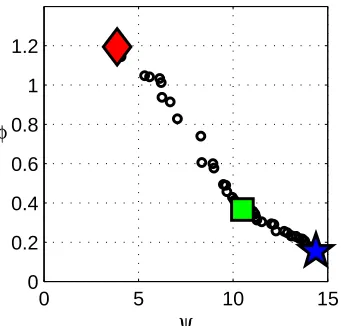
The final approximated set and approximated front are depicted in Fig. 5. The results indicate that softer springs achieve better performance in reducing the reaction to the floor’s vibrations, but they are more expensive. Interestingly, the solution with the best damping is not the one with the minimal value of spring coefficient for both springs, but a solution withk1= 1 mmN andk2= 3.5 mmN . This difference
has shown to decrease the equipment’s displacement better than two springs with an equal coefficient of 1 N
mm.
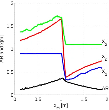
The AR and adjustments of three solutions as a function of
xmare depicted in Fig. 6. These three solutions are highlighted
in Fig. 5 as a square, a star and a diamond. Fig. 6(a)–6(c) depict the AR and optimal locations of springs and damper for each of the three solutions, and Fig. 6(d) depicts the optimal damping coefficients. Note that solutions with stiffer springs, in addition to their lower cost, require smaller adjustments to changes in location of the experimental equipment. Another interesting observation is that the optimal adjustments of the damper and components’ locations for the star related solution are not symmetric. This is a consequence of the differences between its springs.
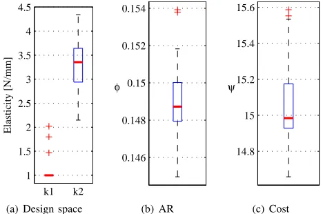
In order to assess the reliability of the obtained approxi-mated front, the problem was solved for twenty independent runs of the EA. The statistics for the solution with the best AR (marked with a star in Fig. 5) is depicted in Fig. 7.
To check the added value of adaptation to the performance of the adaptive optical table, it is compared with a similar design that is not adaptive. This design possesses the same characteristics, but it cannot be changed once implemented (i.e., all its variables are of type x). The costs are not considered for this comparison, and the only consideration is minimal AR. The optimal non-adaptive product is found by solving the following worst-case RO problem:
xna= argmin
x∈X
max
p∈P
AR(x,p) (31)
wherex= [k1, k2, c, xc, x1, x2],p= [m, xm, ω, M, L], andP
and the limits of X are the same as for the AROP.
The solution to the problem in (31) is xna =
[1,1,1,1,0.9,1.1], i.e., both springs and the damper are the weakest possible, the damper is located at the center of the table, and the springs are as close to the center as possible.
1 1.5 2 2.5 3 3.5 4 4.5
k1 k2
Elasticity [N/mm]
(a) Design space
0.146 0.148 0.15 0.152 0.154
φ
(b) AR
14.8 15 15.2 15.4 15.6
ψ
[image:10.612.331.565.52.207.2](c) Cost
Fig. 7. Box-plots for the results of the obtained adaptive solution with the best AR, from 20 independent simulations of the EA.
The maximal AR for this configuration occurs when the center of mass aligns with the center of the table, and its value is
ϕ(xna) = 0.456. This value is three times higher than the
worst AR of the adaptive solutionx⋆, which isϕ(
x⋆)
= 0.15.
V. CONCLUSIONS ANDFUTUREWORK
In this paperActive Robustness, a novel robust optimization approach, was introduced. With this approach, robustness is enhanced by adaptation to a possibly changing environment. The Active Robust Optimization Problem was formulated. The AROP motivates a search for cost effective adaptive solutions, by simultaneously optimizing for high performance and low cost. During the design phase, the possible scenarios of the uncertainties involved are considered, and the optimal configuration for a sampled set of scenarios is searched for. It was shown that an adaptive solution that possesses active robustness is able to achieve better performance than an equivalent non-adaptive solution.
The type of uncertainty treated in the framework of this paper was a dynamic or uncertain environment. However, the AROP is not limited to this type alone, and can be easily adopted to deal with other sources of uncertainties. If the fixed design variables are subjected to uncertainties (e.g., as a result of manufacturing tolerances or deterioration), then these uncertainties can be considered when solving (8). In a similar manner, if the adjustable variables cannot be precisely determined (e.g., due to control issues), the variation of Y⋆
from its desired value can also be added as an uncertain parameter to (8).
0 50 100 0
20 40 60 80 100
k
1 [N/mm] k 2
[N/mm]
(a) The obtained approximated Pareto optimal set. The spring coefficients of the three highlighted solutions are:
x⋆= [1,3.7] N
mm, x
= [15,14] N
mm, and x =
[96,96] N mm.
0 5 10 15
0 0.2 0.4 0.6 0.8 1 1.2
ψ φ
[image:11.612.333.504.63.226.2](b) The obtained approximated Pareto front. The solution with the minimal AR is marked with a star, the solution with the lowest cost is marked with a diamond, and a trade-off solution is marked with a square.
Fig. 5. Final approximated set and Pareto front after 50 generations of the evolutionary algorithm.
within the AROP, as the performance and cost of each solution are evaluated according to its own adjustable domain.
The main drawback of the AROP is its high complexity. This complexity can be easily noticed by examining the algorithm suggested in Section III-C: Assuming the DOP of (8) (Steps 9– 11), is solved by an EA with a population size n and G
generations; then nG function evaluations are conducted for each sample of the environmental space. If the environmental space is sampledktimes; then the DOP requiresnGkfunction evaluations for each solution x. Assuming the MOP of (7) is also terminated after G generations, and has a population size of n; then the total number of function evaluations will be n2G2k. In addition, the cost function has to be evaluated as well nG times. A variety of methods exist for reducing the number of function evaluations in Algorithm 1 or using approximation methods in the case of expensive functions (for a comprehensive survey see [16]). An important future work, in order to allow for practical implementation of the AROP in real life applications, will be to implement these methods.
Another future work is to further investigate the adaptation’s cost of the AROP (cp). The adaptation’s cost suggested here only considers the resources required for adaptation (reflected from the differences between optimal configurations). In [17], a method to optimize adaptation to a given environmental change was introduced. There, in addition to the resources required for adaptation, the performance of the solution during adaptation is also considered. An integration of this method into the AROP might result in a more accurate evaluation of the solution’s active robustness.
The suggested AROP is a two-stage optimization problem, where the first stage (Equation (8)) considers the solution’s best performance for each scenario, and the second stage (Equa-tion (7)) considers the performance–cost trade-off between candidate solutions. Since the main goals are performance
and cost, it is conceivable to evaluate a solution according to these two goals in the first stage as well. If this is the case, Equation (8) needs to be reformulated to the following dynamic MOP:
Y⋆= argmin
y∈Y(x)
Z= [F(x,y,P), Cy(x,y,P)] (32)
This means that a solution would be assessed according to sub-optimal configurations if they contribute to reducing its operational costs (cy). In contrast to the one-to-one mapping of (8) between each environmental scenario and its optimal configuration, here each scenario would be associated with a set of Pareto optimal configurations. As a result the objective functions’ variateF andC should be evaluated according to a set-based approach. As a future work, the pros and cons of the extended formulation of the AROP should be studied.
So far, the AROP deals with cases where there is only a single objective function. The next stage of this study would deal with generalizing the AROP to enhance robustness of solutions to multiobjective problems. In a MOP, the best performances of an adaptive solution, for every realization of the uncertainties, is a set of Pareto optimal configurations. Therefore, we envisage that a set-based approach for evaluating the solutions’ performances would be required.
ACKNOWLEDGEMENT
This research was supported by a Marie Curie Interna-tional Research Staff Exchange Scheme Fellowship within
the 7th European Community Framework Programme. The
0 0.5 1 1.5 2 0
0.5 1 1.5 2
x
m [m]
AR and x[m] xc
x
1
x
2
AR
(a) AR and locations of the components ofx for the various location of the equipment.
0 0.5 1 1.5 2
0 0.5 1 1.5 2
x
m [m]
AR and x[m]
x
c
x
1
x
2
AR
(b) AR and locations of the components ofx for the various location of the equipment.
0 0.5 1 1.5 2
0 0.5 1 1.5 2
x
m [m]
AR and x[m] xc
x
1
x
2
AR
(c) AR and locations of the components of x⋆ for the various location of the equipment.
0 0.5 1 1.5 2
0 2 4 6 8 10
xm [m]
c [Ns/mm]
[image:12.612.112.288.55.233.2](d) Optimal damping coefficients for every location of the equipment. The values for each solution are marked with the solution’s associated shape.
Fig. 6. TheARandY⋆of the highlighted three solutions.
REFERENCES
[1] I. Paenke, J. Branke, and Y. Jin, “Efficient search for robust solutions by means of evolutionary algorithms and fitness approximation,” Evo-lutionary Computation, IEEE Transactions on, vol. 10, no. 4, pp. 405 –420, aug. 2006.
[2] M. S. Phadke,Quality Engineering Using Robust Design, 1st ed. Upper Saddle River, NJ, USA: Prentice Hall PTR, 1995.
[3] J. Branke and J. Rosenbusch, “New approaches to coevolutionary worst-case optimization,” in Parallel Problem Solving from Nature PPSN X, ser. Lecture Notes in Computer Science, G. Rudolph, T. Jansen, S. Lucas, C. Poloni, and N. Beume, Eds. Springer Berlin Heidelberg, 2008, vol. 5199, pp. 144–153.
[4] C. Cruz, J. R. Gonz´alez, and D. A. Pelta, “Optimization in dynamic environments: a survey on problems, methods and measures,” Soft Computing, vol. 15, pp. 1427–1448, 2011.
[5] Y. Koren, U. Heisel, F. Jovane, T. Moriwaki, G. Pritschow, G. Ulsoy, and
H. V. Brussel, “Reconfigurable manufacturing systems,”CIRP Annals - Manufacturing Technology, vol. 48, no. 2, pp. 527 – 540, 1999. [6] P. Gu, M. Hashemian, and A. Nee, “Adaptable design,”CIRP Annals
-Manufacturing Technology, vol. 53, no. 2, pp. 539 – 557, 2004. [7] D. Xue, G. Hua, V. Mehrad, and P. Gu, “Optimal adaptable design
for creating the changeable product based on changeable requirements considering the whole product life-cycle,” Journal of Manufacturing Systems, vol. 31, no. 1, pp. 59 – 68, 2012.
[8] A. Ben-Tal, A. Goryashko, E. Guslitzer, and A. Nemirovski, “Adjustable robust solutions of uncertain linear programs,”Mathematical Program-ming, vol. 99, no. 2, pp. 351–376, 2004.
[9] D. Bertsimas, V. Goyal, and X. Sun, “A geometric characterization of the power of finite adaptability in multistage stochastic and adaptive optimization,”Mathematics of Operations Research, vol. 36, no. 1, pp. 24–54, 2011.
formula-tion and search by way of evoluformula-tionary multi-objective optimizaformula-tion,”
Engineering Optimization, vol. 42, no. 5, pp. 453–470, 2010. [11] M. D. McKay, R. J. Beckman, and W. J. Conover, “Comparison of three
methods for selecting values of input variables in the analysis of output from a computer code,”Technometrics, vol. 21, no. 2, pp. 239–245, 1979.
[12] Newport Corporation. Vibration control - identifying and controlling vibrations in the workplace. [Online]. Avail-able: http://photonics.com/edu/Handbook.aspx?AID=25517 [Accessed: 29.01.2013]
[13] S. Salomon, G. Avigad, A. Goldvard, and O. Sch¨utze, “PSA a new scalable space partition based selection algorithm for MOEAs,” in
EVOLVE - A Bridge between Probability, Set Oriented Numerics, and Evolutionary Computation II, ser. Advances in Intelligent Systems and Computing, O. Sch¨utze, Ed. Springer Berlin Heidelberg, 2013, vol. 175, pp. 137–151.
[14] C. Mattson and A. Messac, “Pareto frontier based concept selection under uncertainty, with visualization,”Optimization and Engineering, vol. 6, no. 1, pp. 85–115, 2005.
[15] G. Avigad and A. Moshaiov, “Simultaneous concept-based evolutionary multi-objective optimization,”Applied Soft Computing, vol. 11, no. 1, pp. 193 – 207, 2011.
[16] Y. Jin, S. Member, and J. Branke, “Evolutionary Optimization in Uncertain Environments A Survey,”Evolutionary Computation, IEEE Transactions on, vol. 9, no. 3, pp. 303–317, 2005.