Selecting precise reference normal tissue samples for cancer research using a deep learning approach

R E S E A R C H

Open Access

Selecting precise reference normal tissue

samples for cancer research using a deep

learning approach

William Z. D. Zeng

, Benjamin S. Glicksberg

, Yangyan Li

and Bin Chen

FromThe International Conference on Intelligent Biology and Medicine (ICIBM) 2018 Los Angeles, CA, USA. 10-12 June 2018

Abstract

Background:Normal tissue samples are often employed as a control for understanding disease mechanisms, however, collecting matched normal tissues from patients is difficult in many instances. In cancer research, for example, the open cancer resources such as TCGA and TARGET do not provide matched tissue samples for every cancer or cancer subtype. The recent GTEx project has profiled samples from healthy individuals, providing an excellent resource for this field, yet the feasibility of using GTEx samples as the reference remains unanswered.

Methods:We analyze RNA-Seq data processed from the same computational pipeline and systematically evaluate GTEx as a potential reference resource. We use those cancers that have adjacent normal tissues in TCGA as a benchmark for the evaluation. To correlate tumor samples and normal samples, we explore top varying genes, reduced features from principal component analysis, and encoded features from an autoencoder neural network. We first evaluate whether these methods can identify the correct tissue of origin from GTEx for a given cancer and then seek to answer whether disease expression signatures are consistent between those derived from TCGA and from GTEx.

Results:Among 32 TCGA cancers, 18 cancers have less than 10 matched adjacent normal tissue samples. Among three methods, autoencoder performed the best in predicting tissue of origin, with 12 of 14 cancers correctly predicted. The reason for misclassification of two cancers is that none of normal samples from GTEx correlate well with any tumor samples in these cancers. This suggests that GTEx has matched tissues for the majority cancers, but not all. While using autoencoder to select proper normal samples for disease signature creation, we found that disease signatures derived from normal samples selected via an autoencoder from GTEx are consistent with those derived from adjacent samples from TCGA in many cases. Interestingly, choosing top 50 mostly correlated samples regardless of tissue type performed reasonably well or even better in some cancers.

Conclusions:Our findings demonstrate that samples from GTEx can serve as reference normal samples for cancers, especially those do not have available adjacent tissue samples. A deep-learning based approach holds promise to select proper normal samples.

Keywords:Drug repositioning, Deep learning, Autoencoder, Disease signatures

* Correspondence:[email protected]

1_{Institute for Computational Health Sciences, University of California, San} Francisco, CA, USA

3_{Department of Pediatrics and Human Development, Department of} Pharmacology and Toxicology, Michigan State University, 15 Michigan St. NE, Grand Rapids, MI 49503, USA

Full list of author information is available at the end of the article

Background

Comparing molecular profiles of disease tissue samples and normal tissue samples is often employed to identify a signature of the disease. The signature defined as dif-ferentially expressed genes between two groups is critical to understanding abnormal disease features and guiding therapeutic discovery [1–6]. For example, a gene expres-sion signature created from the comparison of liver can-cer tumor samples and adjacent tissue samples was used to discover anti-parasite drugs as therapeutics for liver cancer [7]. Analysis of matched tumor and normal pro-files identified common transcriptional and epigenetic signals shared across cancer types [8]. Large-scale inte-grative analysis of cancer profiles, cellular response sig-natures and pharmacogenomics data suggested that such disease signatures can be widely employed for screening anti-cancer drugs [9].

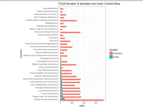
However, there are many lingering issues that hinder these types of analyses. For instance, in many cancers, adjacent normal tissues are not available in these gen-omic databases such as The Cancer Genome Atlas (TCGA) and Therapeutically Applicable Research To

Generate Effective Treatments (TARGET) (Fig. 1). As such, there is an open question on what tissue samples should be selected for these scenarios or whether cre-ation of a proper disease signature is even possible. The recent Genotype-Tissue Expression (GTEx) project [10] has profiled samples from healthy individuals, providing an excellent resource. However, their profiles are gener-ated from different studies and processed under different computational approaches, the feasibility of using GTEx samples as the reference remains unanswered. Moreover, given the fact there is heterogeneity within a disease, an-other goal is to determine a set of normal samples that are optimal for use as the reference for a group of pa-tient samples. One approach is to choose normal sam-ples that are similar to disease samsam-ples based on their gene expression profiles. As a substantial number of genes that are lowly expressed or not expressed at all add noises in similarity measurement, one typical alter-native strategy is to utilize the top varying genes across disease samples as the features for similarity measure-ment. However, selecting top varying genes may ignore information of many critical genes.

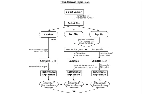
In this work, we use the RNA-Seq data processed from the UC Santa Cruz Computational Genomics Lab’s Toil-based RNA-seq pipeline [11] and systematically evaluate GTEx as a potential reference resource (Fig.2). We use those cancers that have adjacent normal tissues in TCGA as the benchmark for the evaluation. We also explore the potential use for state-of-the-art deep learn-ing models, specifically layers of autoencoders, to create reduced features for similarity measurement. We found that disease signatures derived from normal samples in GTEx are consistent with those derived from adjacent samples in TCGA in many cases. Our findings demon-strate that samples from GTEx can serve as reference samples for the majority of cancers, but not all. Add-itionally, we show promising results for utilizing deep learning strategies to select reference tissues.

Methods Datasets

TCGA (https://cancergenome.nih.gov/) is a public re-pository of genomics data (e.g., gene expression) for can-cer, and sometimes adjacent normal tissues. TARGET is a similar resource focused on childhood cancers. The GTEx project is a collection of gene expression data for over 7700 healthy individuals for over 50 tissues. In the

current study, raw counts data and phenotype metadata for the analysis were downloaded from UCSC Xena Treehouse (https://xenabrowser.net/datapages/?cohort= TCGA%20TARGET%20GTEx) and processed into an R dataframe consisting of studies from TCGA, TARGET, and GTEx, with a total of 58,581 rows of gene expres-sion raw counts (identified as HUGO gene symbols). Transcript abundance estimated from STAR and RSEM was used. The Treehouse raw counts data consist of 19,249 samples and, of those, a total of 19,131 tissue samples were annotated with phenotype metadata. We only used tissue samples with annotated metadata for this analysis. Of the 32 cancers, we chose cancers that have at least 10 case-control (tumor-adjacent normal) sample pairs (Fig.1).

Workflow

In our study, we first evaluate whether our approach can identify the correct tissue site from GTEx for a given cancer (Fig. 2). We then ask whether disease signatures are consistent between those derived from TCGA and from GTEx. First we selected tissues for a particular can-cer in the TCGA dataset and performed quality control by filtering for tumor purity > 0.7 as determined by ES-TIMATE [12]. Tissue outliers were determined by

computing the principal component analysis of tissues and filtering out those with absolute z-score of the first component of greater than 3. Reference normal tissue for the tumor samples were computed using four methods:

a. Random Method: Random selection of 50 GTEx normal tissues.

b. Top Site Method: Compute correlation of GTEx tissue expression to tumor expression using top 5000 varying genes across all tumors and select all tissue samples from the top correlating tissue site. Alternatively, compute correlation using the features calculated from an autoencoder.

c. Top 50 tissues method: Compute correlation of each GTEx tissue expression to tumor expression and select the site with the tissues of the 50 highest correlation to the tumor samples.

d. Manual method: For certain tumor tissues where the computed top site did not correspond to the site of tumor. For example, if esophagus mucosa was chosen for lung adenocarcinoma, we manually selected GTEx tissue site - lung.

After the reference GTEx tissues were selected, we again removed tissues for outliers based on computed first PCA > 3. Then the tumor tissues and reference tis-sues were normalized using the RUVg R package library [13]. Differential expression was computed on the nor-malized samples. We analyzed each differential expres-sion of the computations by comparing it with differential expressions computed from case-control set. The signature genes selected for analysis had an absolute log fold change of greater than 1 and adjustedp-value of less than 0.001.

First, we performed differential expression analysis by comparing tumor samples and normal samples using edgeR [14]. While we chose edgeR only to use, our pre-liminary assessment showed the conclusions hold using Limma + voom [15] or DESeq [16]. We filtered for can-cers where there were at least 10 pairs of case-control samples. These were Breast Invasive Carcinoma, Kidney Clear Cell Carcinoma, Thyroid Carcinoma, Lung Adeno-carcinoma, Prostate AdenoAdeno-carcinoma, Liver Hepatocel-lular Carcinoma, Lung Squamous Cell Carcinoma, Head & Neck Squamous Cell Carcinoma, Stomach Adenocar-cinoma, Kidney Papillary Cell CarAdenocar-cinoma, Colon Adeno-carcinoma, Kidney Chromophobe, Bladder Urothelial Carcinoma, Esophageal Carcinoma. The differential ex-pression computed from these case-control cancer sam-ples was used as benchmark comparison to the differential expression ran against GTEx tissues as se-lected from the workflow (Fig. 2). To evaluate the performance we computed consistency based on the

significance of overlaping genes between signatures and correlation of fold changes of common signature genes. Further, disease expression using GTEx reference tissues were computed as in the workflow diagram. All the ana-lyses were performed in R (version 3.4.3).

Autoencoder

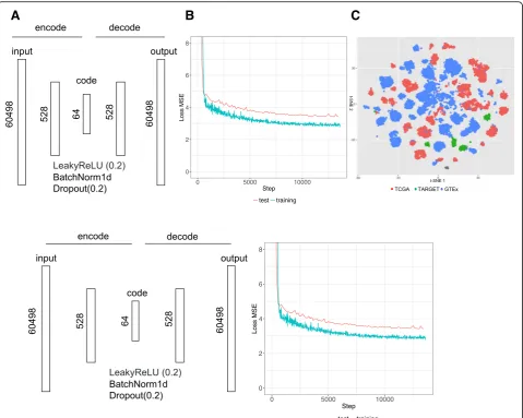
As an alternative approach to the top site methods, we evaluated the utility of an autoencoder neural network for computing correlation between cancer and reference tissue expression. Gene counts in terms of Transcripts Per Kilobase Million (TPM) from 19,260 samples were fed into an autoencoder implemented using Pytorch (v. 0.1.12_2) (http://pytorch.org/). The following parameters were used: 64 encoded features, 128 batch size, 100 epochs, 0.0002 learning rate (Fig. 3a). The training took about 30 min using one GPU in an Amazon cloud (g3.8xlarge). Rectifying activation function, dropout and normalization were applied between layers. The loss function is defined as a mean squared error (MSE) be-tween 60,498 elements (identified as Ensembl IDs) in the input x and output y. The functions and parameters were detailed on the PyTorch website ( https://pytorch.-org/docs/master/). Data were split into a training set (80%) and a test set (20%). Loss converged after 10,000 iterations (Fig. 3b). The t-SNE plot of the reduced data-set shows that batch effect among three databases was minimized (Fig. 3c). Similarly, we performed principal component analysis (PCA) of this datasets and chose top 64 components as the features. As the top 64 com-ponents could explain 92% variation, choosing 64 fea-tures for similarity measurement is reasonable in both autoencoder and PCA.

Results

Among 32 TCGA cancers, 18 cancers have less than 10 matched adjacent normal tissue samples in the Tree-house dataset. Ten cancers do not have any matched ad-jacent tissue samples at all (Fig. 1). Whereas, GTEx has profiles for 47 tissue sites with at least ten normal sam-ples. This suggests the significance of exploring GTEx as a source of reference.

Computing tissue of origin

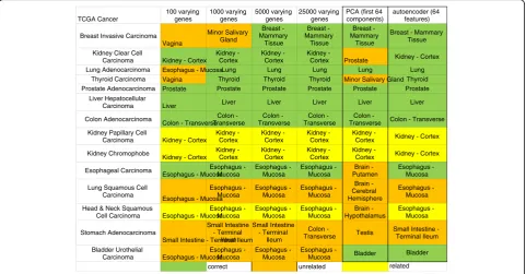
number of varying genes to 5000 improved correct se-lection for 11 of 14 cancers. No further improvement on tissue selection was seen by increasing number of vary-ing genes. The PCA, as a regular dimension reduction method, was only able to correctly identify 8 of 14 can-cers, so we did not examine this method in the following analysis. The best automated method we found for refer-ence tissue selection was via correlating autoencoder features with 12 of 14 tissues being correctly chosen.

Further examination of the three misclassified cancers by varying genes methods, Bladder Urothelial Carcin-oma, Lung Squamous Cell Carcinoma and Stomach Adenocarcinoma, revealed correlation values of 0.549,

0.300, and 0.858, respectively. The low correlation from the bladder and lung carcinoma may be due to substan-tial difference in tissue expression between the com-puted site, esophagus, and their expected origin site, bladder and lung. Correlation for stomach adenocarcin-oma was quite high, which may be due to similarity be-tween the computed site, ileum of the small intestine, and the stomach (Additional file1: Table S1).

Squamous cell carcinomas arise from squamous cells that reside in the cavities and surfaces of blood vessels and organs. As samples in GTEx were taken from bulk tissues, this may cause the lower computed correlation between the cancer tissue and site of origin leading to

A

B

C

erratic computational choices. Manual selection of the tissue of origin for lung squamous cell carcinoma and stomach adenocarcinoma improved the correlation from 0.549 and 0.858 to 0.883 and 0.926 respectively (Additional file 1: Table S1). For Bladder Urothelial Carcinoma, using the varying genes method chose esophagus - mucosa as the top site (correlation 0.549), whereas autoencoder correctly chose the bladder site (correlation 0.926). This shows that correct site choices will improve correlation.

Interestingly, Kidney Clear Cell Carcinoma, Kidney Papillary Cell Carcinoma and Kidney Chromophobe share the same tissue origin--Kidney - Cortex. This con-firms that cancer can arise from different parts of one tissue and raise the question whether we should use all normal samples from one site as the reference.

Examples of hepatocellular carcinoma and bladder urothelial carcinoma

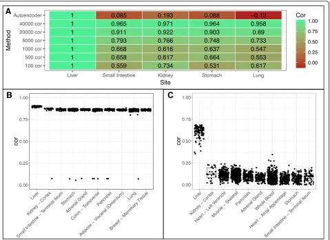
We use two cancers as examples for further in-depth analyses, specifically Hepatocellular Carcinoma (HCC) and Bladder Urothelial Carcinoma (BUC). In our prior results, we found that using more genes to compute the correlation generally helped to select the correct tissue site for the tumor. We ran correlation for each site using increasing number of varying genes as well as autoenco-der features. We normalized the correlation of the can-cer site liver (Fig. 5a). We found that as the number of genes used increases all tissues will generally converge to have higher correlation with the disease tissue, this

may be due to including genes of conserved regions or low expressions. Using all features from the autoencoder allows us to have much better separation of the site liver from other non-related sites of the cancer, indicating autoencoder captures the biology of disease sample more specifically (Fig.5b-c).

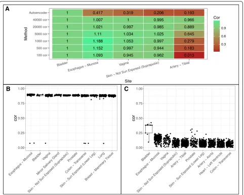
For BUC, however, the varying genes method was un-able to determine bladder as the best site instead choos-ing esophagus (Fig.6a-b). Increasing varying genes from 100 to 40,000 brought down the correlation of esopha-gus site relative to bladder, however, it brought up cor-relation of other tissue sites relative to bladder (Fig. 6a) similar to what we see in Fig. 5a. This suggests that naively increasing varying genes does not help to distin-guish tissue site selection. Meanwhile, the autoencoder method correctly predicts bladder as the top site with great separation between bladder and esophagus (Fig.6a, c). Notably, the correlation in BUC is lower than that in HCC based on different similarity metrics. This suggests that cell composition in bladder tissues may be more diverse.

Disease signature comparison

As we have demonstrated that gene expression profiles can be used to identify tissue of origin, we then asked if these samples sharing the same tissue of origin from GTEx can substitute adjacent tissues from TCGA to cre-ate disease signatures. We employed three approaches to select samples (Fig. 2). We evaluate consistency based

TCGA Cancer 100 varying genes 1000 varying genes 5000 varying genes 25000 varying genes

PCA (first 64 components)

autoencoder (64 features)

Breast Invasive Carcinoma Vagina Minor Salivary Gland Breast - Mammary Tissue Breast - Mammary Tissue Breast - Mammary Tissue

Breast - Mammary Tissue

Kidney Clear Cell

Carcinoma Kidney - Cortex Kidney -

Cortex

Kidney - Cortex

Kidney -

Cortex Prostate Kidney - Cortex

Lung Adenocarcinoma Esophagus - MucosaLung Lung Lung Lung Lung

Thyroid Carcinoma Vagina Thyroid Thyroid Thyroid Minor Salivary Gland Thyroid

Prostate Adenocarcinoma Prostate Prostate Prostate Prostate Prostate Prostate

Liver Hepatocellular

Carcinoma Liver Liver Liver Liver Liver Liver

Colon Adenocarcinoma

Colon - Transverse Colon - Transverse Colon - Transverse Colon - Transverse Colon

-Transverse Colon - Transverse Kidney Papillary Cell

Carcinoma Kidney - Cortex Kidney - Cortex Kidney - Cortex Kidney - Cortex Kidney -

Cortex Kidney - Cortex

Kidney Chromophobe

Kidney - Cortex Kidney - Cortex Kidney - Cortex Kidney - Cortex Kidney -

Cortex Kidney - Cortex

Esophageal Carcinoma

Esophagus - Mucosa Esophagus - Mucosa Esophagus - Mucosa Esophagus - Mucosa Brain - Putamen Esophagus - Mucosa

Lung Squamous Cell Carcinoma

Esophagus - Mucosa Esophagus - Mucosa Esophagus - Mucosa Esophagus - Mucosa Brain - Cerebral Hemisphere Esophagus - Mucosa

Head & Neck Squamous

Cell Carcinoma Esophagus - Mucosa Esophagus - Mucosa Esophagus - Mucosa Esophagus - Mucosa Brain - Hypothalamus Esophagus - Mucosa Stomach Adenocarcinoma

Small Intestine - Terminal Ileum Small Intestine - Terminal Ileum Small Intestine - Terminal Ileum Colon - Transverse Testis

Small Intestine - Terminal Ileum

Bladder Urothelial

Carcinoma Esophagus - Mucosa Esophagus - Mucosa Esophagus - Mucosa Esophagus - Mucosa Bladder correct unrelated Bladder related

on the significance of overlap between signatures and correlation of fold changes of common signature genes.

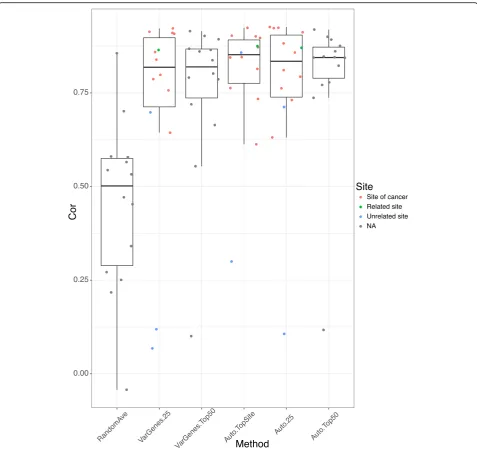
Figure7 shows the rank-based correlation of differen-tial expression between consensus transcripts for each cancer from TCGA using GTEx reference tissue vs. TCGA case-control samples. Using the average of three random tissue site selection as our baseline we see that our other strategies are superior. The autoencoder pro-duced better correlations overall regardless of sample se-lection method.

For the autoencoder, it seems that choosing all sam-ples from the same tissue of origin performs slightly better than choosing 25 percentile and above mostly correlated samples from the same tissue of origin. Interestingly, choosing top 50 mostly correlated sam-ples from any tissue performs reasonably well or even better in some cancers, where the tissue of origin was misclassified such as the varying genes method for stomach adenocarcinoma (Additional file 1: Table S1). This is very significant because in many cases, where we may have no or an insufficient number of matched

normal tissues, we may use normal samples from other sites. For example, in the three kidney cancers: Kidney Clear Cell Carcinoma, Kidney Papillary Cell Carcinoma and Kidney Chromophobe, our analysis suggests three cancers can share the same reference tissue sites des-pite the differences of origin within the kidney.

One additional question we assessed is how many normal samples are sufficient for proper disease signature-related analyses? We found that even a rela-tively low number of normal samples may be sufficient for calculating differential expression. For bladder urothelial cancer, for example, the autoencoder se-lected the bladder GTEx site which consists of only nine tissue samples (Fig. 1) for a correlation of 0.924; filtering for tissues above the 25th percentile left only seven tissue samples for a correlation of 0.926. When we used a strategy that selected more tissues, i.e. using autoencoder top 50 method, 50 sample tissues were used (9 from bladder and 41 from other top correlated sites), which produced a slight drop of correlation to 0.847. This indicates that even a relatively low number

A

B

C

of reference tissue samples may provide a robust match.

Finally, we assessed whether it is a better strategy overall to select all samples from the same tissue site as the cancer of interest or only those that are correlated to the tumor sample. We found that the samples producing the best performance are sites where the tumor devel-oped or closely related sites. However, when it is not possible to use such sites (e.g., when there are no avail-able data), it is feasible to use top correlated tissues as seen from the top 50 methods. However, we found that for some cancers, even choosing top correlated sites can still produce erratic results, such as in the case of lung squamous cell cancer. In this case, the correlations for all non-random methods were between 0.1–0.3 which was not even able to beat the random tissue selection (Additional file 1: Table S1). Along these lines, we evaluated differential expression similarity using samples

from a different origin than the cancer of interest. For example, in two kidney cancers, Kidney Papillary Carcinoma and Kidney Chromophobe the kidney cor-tex were computed as the top site, for Head and Neck carcinoma the esophagus-mucosa was the top site. Their high correlation with case-control > 0.8 indicates that choosing sites at different origin but proximal to the cancer will provide good disease signa-tures (Additional file1: Table S1).

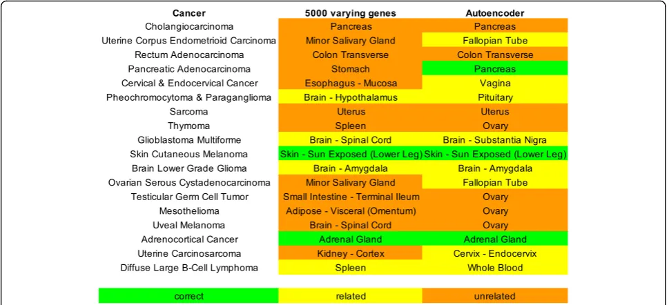
Assign normal tissues for cancers with low case-control pairs

Since there were 18 cancers with insufficient number of adjacent normal tissues, we use our computational ap-proach to assign a primary site for each. Of the 18 can-cers, the autoencoder method was able to determine 10 correct sites, whereas using the top 5000 varying genes only produced 4 correct sites (Fig. 8). This suggests an

A

B

C

autoencoder can select proper samples to create disease signatures for those cancers.

Discussion

As the cost of sequencing is rapidly decreasing, it be-comes very common to profile disease samples of interest, however, collecting matched normal tissues from patients is difficult in many instances. Our ana-lysis confirms that GTEx, the largest cohort of normal samples, can serve as a source of reference normal tis-sues in cancer research. In the current study, we chose

to focus on cancer because we have plenty of adjacent tissues that can be used as a benchmark. We expect that the methods and findings from our study can be extended for cancer subtypes or other non-cancer re-search as well.

However, a few caveats have to be considered. First, all RNA Seq data have to be processed in the same pipeline in order to mitigate batch effects. Second, some disease samples may have no relevant normal tissue samples in GTEx because of diverse cellular composition. This limita-tion may be addressed by using cellular decomposilimita-tion

techniques or single cell data. Finally, although we show the potential of using autoencoder for feature se-lection, we have not fully optimized the model for tis-sue selection. In our exploratory studies, we found that encoded features are very sensitive to network architecture and parameters, although it does not affect the results in the computation of tissue of ori-gin. For example, when we changed learning rate from 0.0002 to 0.005, batch size from 128 to 64, dropout rate from 0.2 to 0.1, LeakyReLU negative slope from 0.2 to 0.1, respectively, the average correlation be-tween the new features and the default features chan-ged to 0.219, 0.069, 0.354, and 0.219 (Additional file2: Table S1). Interestingly, while a new layer was added into the network, the average correlation even de-creased to −0.01. However, while using new features to compute tissue of origin, we observed that all new features could clearly separate the first top site and the second top site. For example, in liver and bladder cancers, liver and bladder are predicted as the top site respectively, and the correlation with the top site is much higher than that with the second site (Add-itional file 2: Table S1). Surprisingly, when the feature size was reduced from 64 and 32 or two new layers were added, the top site of bladder cancer was incor-rectly predicted.

In addition, we identified several steps to further ex-plore. For instance we may include additional genomic features such as of mutations and copy number vari-ation. The autoencoder strategy would be able to man-age such diverse feature types. We also plan to determine whether changing the order of workflow, such as removing outliers first, might improve this analysis. In

addition, as adjacent cancer normal tissues are sampled near the cancer site, some of these tissues may contain cancer cells and thus have some expression of cancer [17], which may require further investigation. We will further explore our approach to study cancer subtypes (estrogen-receptor positive breast cancer) and pediatric cancers (available in TARGET), where adjacent normal tissues are even more scarce.

Conclusion

In the current study, we evaluated the nuances of proper reference tissue selection for disease signature-related analyses. We showed that we can compute differentially expressed genes in cancer by comparing cancer tissues to reference tissues from the same site even if they are from a different database. Furthermore, we assessed the benefit of using state-of-the-art methodologies, namely deep learning via an autoencoder strategy. We showed that it enhances performance of identifying ideal refer-ence tissues for cancers of interest. The findings from our study will significantly enhance probing disease biol-ogy through gene signatures.

Additional files

Additional file 1:Table S1.Consensus sequence and gene rank correlation with case-control pairs using different methods. Differentially expressed genes were selected using adjustedp< 0.001 and absolute log fold change > 1. Consensus sequences are defined as overlapping differential expression sequences with same directionality in log fold change. Rank correlation is the Spearman’s rank correlation of differential expression (fold change) between the consensus sequences computed from multiple methods (see workflow) and case-control pairs. Unless otherwise stated all rank correlation havepvalues < 0.01. (XLSX 11 kb)

Additional file 2:Table S1.Autoencoder architecture and parameter evaluation. New encoded features were used to compute tissue of origin. A better separation between the first top site and the second top site indicates a better model. (XLSX 8 kb)

Abbreviations

BUC:Bladder Urothelial Carcinoma; GTEx: Genotype-Tissue Expression project; HCC: Hepatocellular Carcinoma; PCA: Principal component analysis; RNA-seq: RNA sequencing; TARGET: Therapeutically Applicable Research To Generate Effective Treatments; TCGA: The Cancer Genome Atlas

Acknowledgements

Not applicable

Funding

The research and publication of this article is supported by R21 TR001743 and K01 ES028047. The content is solely the responsibility of the authors and does not necessarily represent the official views of the National Institutes of Health.

Availability of data and materials

Data and code will be available upon request.

About this supplement

This article has been published as part ofBMC Medical Genomics Volume 12 Supplement 1, 2019: Selected articles from the International Conference on Intelligent Biology and Medicine (ICIBM) 2018: medical genomics.The full contents of the supplement are available online athttps://bmcmedgeno mics.biomedcentral.com/articles/supplements/volume-12-supplement-1.

Authors_’contributions

WZ and BC conceived the study. WZ performed the majority of analysis with the input from BSG and BC. YL and BC implemented the deep learning infrastructure. WZ, BSG, and BC wrote the manuscript with the input from YL. BC supervised the study. All of the authors have read and approved the final manuscript.

Ethics approval and consent to participate

No applicable

Consent for publication

Not applicable

Competing interests

The authors declare that they have no competing interests.

Publisher’s Note

Springer Nature remains neutral with regard to jurisdictional claims in published maps and institutional affiliations.

Author details

1_{Institute for Computational Health Sciences, University of California, San} Francisco, CA, USA.2_{Shandong University, Qingdao, Shandong, China.} 3_{Department of Pediatrics and Human Development, Department of} Pharmacology and Toxicology, Michigan State University, 15 Michigan St. NE, Grand Rapids, MI 49503, USA.

Published: 31 January 2019

References

1. Mirza AN, Fry MA, Urman NM, Atwood SX, Roffey J, Ott GR, Chen B, Lee A, Brown AS, Aasi SZ, et al. Combined inhibition of atypical PKC and histone deacetylase 1 is cooperative in basal cell carcinoma treatment. JCI Insight. 2017;2(21).https://doi.org/10.1172/jci.insight.97071. 2. Sirota M, Dudley JT, Kim J, Chiang AP, Morgan AA, Sweet-Cordero A,

Sage J, Butte AJ. Discovery and preclinical validation of drug indications using compendia of public gene expression data. Sci Transl Med. 2011; 3(96):96ra77.

3. Jahchan NS, Dudley JT, Mazur PK, Flores N, Yang D, Palmerton A, Zmoos AF, Vaka D, Tran KQ, Zhou M, et al. A drug repositioning approach identifies

tricyclic antidepressants as inhibitors of small cell lung cancer and other neuroendocrine tumors. Cancer Discov. 2013;3(12):1364_–77.

4. Pessetto ZY, Chen B, Alturkmani H, Hyter S, Flynn CA, Baltezor M, Ma Y, Rosenthal HG, Neville KA, Weir SJ, et al. In silico and in vitro drug screening identifies new therapeutic approaches for Ewing sarcoma. Oncotarget. 2017; 8(3):4079_–95.

5. Fan-Minogue H, Chen B, Sikora-Wohlfeld W, Sirota M, Butte AJ. A systematic assessment of linking gene expression with genetic variants for prioritizing candidate targets. Pac Symp Biocomput. 2015:383–94.

6. Dudley JT, Sirota M, Shenoy M, Pai RK, Roedder S, Chiang AP, Morgan AA, Sarwal MM, Pasricha PJ, Butte AJ. Computational repositioning of the anticonvulsant topiramate for inflammatory bowel disease. Sci Transl Med. 2011;3(96):96ra76.

7. Chen B, Wei W, Ma L, Yang B, Gill RM, Chua MS, Butte AJ, So S.

Computational discovery of niclosamide ethanolamine, a repurposed drug candidate that reduces growth of hepatocellular carcinoma cells in vitro and in mice by inhibiting cell division cycle 37 signaling. Gastroenterology. 2017;152(8):2022_–36.

8. Gross AM, Kreisberg JF, Ideker T. Analysis of matched tumor and normal profiles reveals common transcriptional and epigenetic signals shared across Cancer types. PLoS One. 2015;10(11):e0142618.

9. Chen B, Ma L, Paik H, Sirota M, Wei W, Chua MS, So S, Butte AJ. Reversal of cancer gene expression correlates with drug efficacy and reveals therapeutic targets. Nat Commun. 2017;8:16022.

10. Consortium GT. The genotype-tissue expression (GTEx) project. Nat Genet. 2013;45(6):580_–5.

11. Vivian J, Rao AA, Nothaft FA, Ketchum C, Armstrong J, Novak A, Pfeil J, Narkizian J, Deran AD, Musselman-Brown A, et al. Toil enables reproducible, open source, big biomedical data analyses. Nat Biotechnol. 2017;35(4):314_–6.

12. Yoshihara K, Shahmoradgoli M, Martinez E, Vegesna R, Kim H, Torres-Garcia W, Trevino V, Shen H, Laird PW, Levine DA, et al. Inferring tumour purity and stromal and immune cell admixture from expression data. Nat Commun. 2013;4:2612.

13. Risso D, Ngai J, Speed TP, Dudoit S. Normalization of RNA-seq data using factor analysis of control genes or samples. Nat Biotechnol. 2014; 32(9):896–902.

14. McCarthy DJ, Chen Y, Smyth GK. Differential expression analysis of multifactor RNA-Seq experiments with respect to biological variation. Nucleic Acids Res. 2012;40(10):4288–97.

15. Law CW, Chen Y, Shi W, Smyth GK. voom: precision weights unlock linear model analysis tools for RNA-seq read counts. Genome Biol. 2014;15(2):R29. 16. Anders S, Huber W. Differential expression analysis for sequence count data.

Genome Biol. 2010;11(10):R106.