promoting access to White Rose research papers
White Rose Research Online
[email protected]
Universities of Leeds, Sheffield and York
http://eprints.whiterose.ac.uk/
This is an author produced version of a paper published in
Proceedings of the
British Machine Vision Conference
White Rose Research Online URL for this paper:
http://eprints.whiterose.ac.uk/75463/
Published paper:
Greenall, J, Hogg, DC and Cohn, AG (2011) Temporal Structure Models for
Event Recognition. Proceedings of the British Machine Vision Conference
BMVC 2011 http://dx.doi.org/10.5244/C.25.62
David C. Hogg
Abstract
In many areas of visual surveillance, the observed activity follows re-occurring pat-terns. This paper demonstrates how such patterns can be exploited to improve the detec-tion rate of independent event detectors. We present a temporal model based on pairwise correlations between event timings, which efficiently exploits limited training data. This is combined with the response from potentially heterogeneous independent event detec-tors to improve the robustness of detections over extended sequences. We demonstrate the efficacy of our system with rigorous testing on a large real-world dataset of aircraft servicing operations. We describe the implementation of a binary classifier based on local histograms of optical flow which is used as the independent event detector in our experiments.
1
Introduction
Throughout this paper we talk about about recognising events within ascenario. In many event recognition domains this notion is quite natural. Television programs are divided into episodes, sports footage is separated into games. Even in domains where video input is continuous such as traffic monitoring, there may be natural ways to divide the footage up i.e. morning commuter rush, midday lull, evening rush etc. Our method is applicable in any domain where such a notion of a scenario is natural, and there exists some repeated temporal structure. This work introduces a novel method for event recognition in structured domains. We define a model for efficiently combining the response from independent event detectors with a prior over the structure of inter-event timings. The model is designed to cope in situations where events of different types can potentially overlap and are not strictly ordered. These are precisely the conditions which cause problems for state-based models such as HMMs that attempt to encode the state of the world at each time step with a latent variable. In our optimization, the temporal midpoints and durations of event instances in a previously unseen sequence are the latent variables to be optimized. Our method, described in Section3, only requires that the timings of at least some of the observed events are loosely correlated. The greater the degree of correlation, the greater the benefit will be; whilst the absence of any free parameters in our model makes it generic and easily applicable to other
c
GREENALL, COHN, HOGG: TSMS FOR EVENT RECOGNTION
domains. We evaluate our method on a large real world dataset, implementing a state of the art activity classification system based on local spatiotemporal features as independent event detectors.
2
Related Work
Previous works on human action recognition can be divided into two broad categories: low-level, which focuses on the recognition of short basic actions normally involving a single participant and high-level, which focuses on recognising compound events involving several actions that are temporally correlated and normally involve multiple participants.
The state of the art methods in the low-level area tend to depend on local spatio-temporal features [4,11]. The most popular datasets in this area have so far consisted of many short clips of actions from different classes: thus mapping the task to a classification problem. There have been some extensions and variations on these kind of methods which go slightly in trying to localize events in time and space [2,5,13]. However, there are few examples in the literature of these architectures being applied to the detection of sparse events in longer sequences.
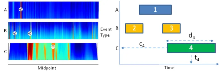
Figure 1: Left: Example response from 3 independent probabilistic event detectors. The detectors give a response for each possible interval in a sequence, with colour indicating the probability (red being high). We show four event instances localized on these likelihood streams. Right: Illustration of corresponding sequence scenario. The scenario is fully speci-fied by event class vectorC= (c1, ...,c4)and temporal informationY= ((t1,d1), ...,(t4,d4)).
on the classification of relatively short actions in isolation. Our approach is complementary to these methods since either of them could be employed as independent event detectors in our system. Our model exploits temporal structure at the inter-event level to make a robust scenario recognition system.
3
Method
3.1
Constructing a Model for Scenario Recognition
Given a previously unseen video sequence of lengthT, we wish to determine the temporal midpoint,t∈T ={1, ..,T}, duration,d∈T, and event class,c∈ {1, ...,M}, of an unknown number,N, of eventinstances, from a fixed vocabulary ofMeventclasses. This is depicted in Figure1(right). The scenario recognition problem over a sequence is challenging since it entails determining the correct number of event instances,N, then optimizating over these 3N random variables. We mitigate the problem of having an unknown N by introducing a‘Null’ state for each(t,d)so that(t,d)∈T2∪Null as a mechanism for ‘switching off’
detections without having to dispose of the corresponding random variables entirely. To simplify matters, for the moment we assume there is at most one event of each type in each sequence. We address the problem of multiple instances of some events in Section
3.4. We are now able to fix the number of event instances in our scenario optimization to beM; fixingC= (c1,c2, ...,cM) = (1,2, ...,M)and leavingY = ((t1,d1), ...,(tM,dM))to be
optimised conditioned onCand the video sequence,X.
We assume that we have already trained a probabilistic event detector for each event class, and that these detectors will be run in parallel to evaluate every possible midpoint and duration over the discrete temporal domain.
Adopting a Bayesian perspective, the output of the independent event detectors can be treated as the likelihood of the relevant chunk of the observed video sequence, X, arising as a result of the given event scenario, which we term p(X|C,Y,θ), where θ is the set
GREENALL, COHN, HOGG: TSMS FOR EVENT RECOGNTION
(ti,di)∈T2. We set the probability of the event beingNull as proportional to the
com-plement of the maximum of the probability of it having occurred at any particular timestep. This enforces a suitable penalty for writing off the output of an event detector as noise and allows us to insert into our model a parameter,αci, for each event class in order to vary the
sensitivity of the detector. In our experiments, we found settingαci= 1 produced results near
to the Equal Error Rate in most cases.
p(X|(ti,di) =Null,ci) =αci(1−max
ti,di
(p(X|(ti,di)∈T2,ci))) (1)
We describe our implementation of a simple but powerful detector based on local spatio-temporal features in Section4.2.
We can then concentrate on optimizing the posterior
p(Y|X,C,θ)∝p(X|C,Y,θ)p(Y|C,θ) (2)
The distribution p(Y|C,θ) denotes the prior probability of a scenario given its event set and the model. By analogy to Pictoral Structure Models [6] from the object detection literature, we define our prior to be a tree-structured Markov Random Field (MRF). The general form for the joint distribution of such a prior can be written
p(Y|C,θ) =∏(i,j)∈E
p((ti,di),(tj,dj)|ci,cj,θ)
∏i∈Vp((ti,di)|ci,θ)degi−1
(3)
where E is the edge set and V the vertices of the MRF. We do not want to give any preference over the absolute timing of any event in isolation, so therefore we setp((ti,di)|ci,θ)to be
uniform, so that Equation3simplifies to.
p(Y|C,θ)∝
∏
(i,j)∈E
p((ti,di),(tj,dj)|ci,cj,θ) (4)
This prior has the following desirable characteristics. Firstly the tree structure ensures that the configuration is to some extent globally consistent since all random variables are (indirectly) connected. Secondly, the distribution is factorized into a product of pairwise terms which should reduce the demands on the amount of training data required to train the model. This is based on the assumption that the training data consists of a number of sequences, each of which contains a subset of the events in our vocabulary. Therefore the higher-order the relationship, the fewer the instances of co-occurrence in the dataset. Finally, the tree-structure allows exact inference on the prior, meaning we can quickly obtain globally optimal solutions.
3.2
Learning Inter-Event Priors
The first component of our prior which must be learnt is the set ofM(M2+1) pairwise proba-bility distributionsp((ti,di),(tj,dj)|ci,cj,θ)which we define to be probability distributions
on the time differences between midpoints of instances of each possible pair of event classes (including the cases whereci=cj) appearing in the same sequence. Note that we omit any
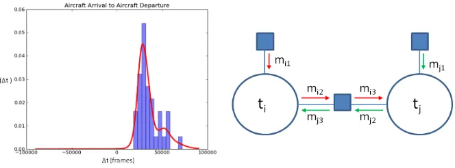
Figure 2: Left: Example of a learnt distribution over the time difference between two event classes in the airport domain. The training data is displayed in the form of a histogram. The distribution on the left is bimodal and skewed, but seems to be well approximated by the learnt distribution plotted in red. This a Gaussian Mixture Model of many overlapping components. Right: Depiction of the message passing scenario between two temporal mid-point random variables. We define the usefulness of the link between i and j to be inversely proportional to the lower of the two entropiesH[mj3],H[mi3]
having studied the data in our test domain, we observed that the single Gaussian is not a good approximator for many of the distributions. In some cases, we observe a distribution that is very skewed, perhaps indicating that one event is supposed to occur soon after another; it can never happen before, yet sometimes it does happen much later. In other cases, there may be two or more distinct modes. A Gaussian Mixture Model (GMM) with a sufficient num-ber of components could model both of these effects. We follow the method of [16], which gives a full Bayesian treatment to the training of GMMs. This approach places a Dirichlet Process prior over the mixture weights of the model, as well as ‘non-informative’ priors over the mean and variance parameters. This way, the number of components is simultaneously optimized with the other parameters in the model. The Dirichlet Process priors make direct optimization intractable, so instead the posterior distribution over the parameter space is ap-proximated through Gibbs sampling. We then use model averaging over 20 samples drawn over 1000 iterations (allowing 50 iterations for burn-in). The result of this procedure is a GMM with a large number of components which are highly-overlapped, but the overhead of evaluating these PDFs can be eliminated at execution time by the use of look-up tables. Figure2(left) gives an example of the kind of distributions learnt by this procedure.
Note that in the previous section we introducedNull states for the(t,d)variables. We now define the joint probability of a ‘switched off’ instance with any other event to be uni-form:
p((ti,di),(tj,dj)|ci,cj,θ) = 1
T;(ti,di) =Nullor(tj,dj) =Null (5)
3.3
Dynamic Structure Assignment
GREENALL, COHN, HOGG: TSMS FOR EVENT RECOGNTION
potential edges in the MRF. As we require our prior to be a tree-structured MRF, and the variables withinY are discrete, the MAP solution to Equation2may be obtained directly through the max-sum Belief Propagation (BP) algorithm [1]. Simplifying the prior to a tree structure will result in the loss of some information, so we need to ensure the edges we retain are the most informative. BP is a message passing algorithm and in this context, we believe it is reasonable to assume the most useful messages will be those of lowest entropy. Therefore to determine the structure of the tree, we evaluate the informativeness of each pairwise connection with the following equation.
I(i,j) =H[p(X|(ti,di),ci,θ)
∑
tj
p(ti,tj|ci,cj,θ)] (6)
which is equivalent to the entropy of the initial message that would be passed fromti totj
(shown in figure2 (right)). Note that this measure factors in the entropy of the detectors’ responses over the sequence, meaning event instances with noisy observation likelihoods over a particular sequence are less likely to be connected to one another. CalculatingIfor each pair of event instances gives aN×N matrix, which we make symmetric by setting
I(i,j)→max(I(i,j),I(j,i)). To this we apply Kruskal’s algorithm [9] to construct the de-sired minimum spanning tree.
3.4
Scenario Recognition with Multiple Instances
In Section3.1we introduced the idea of aNull state to allow us to efficiently deal with the prior uncertainty over whether a particular event occurs within a sequence. Here we discuss our method for coping with the scenario recognition problem in its full generality: where multiple instances of the same event class may occur.
One obvious solution might be to set a hard upper limit on the number of instances of each particular class which could occur within a scenario, then to initialize the appropriate random variables before simply finding the MAP solution as in the single instance case. There is a problem with this approach since we take the observation likelihood for repeat in-stances of the same event class from the same detector. For this reason, we require inin-stances of the same event class to be non-overlapping so that multiple instances don’t point to the same activity. However, this is an impossible constraint to impose with a tree structured prior.
To solve the problem, we use a greedy procedure which is fast and proves to be effective. First we perform our exact optimization of Equation2allowing exactly one instance of each event class. For events which had instances localized successfully ((ti,di)6=Null), we create
an additional instance for the next stage in our optimization. To prevent overlap, we fix the previously localized events by transforming their observation likelihood function to a Dirac delta function and set the observation likelihood of the new instance to zero at all(ti,di)
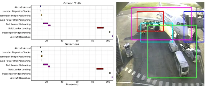
Figure 3: Left: Gantt chart plot showing successful detection results from one of our 37 sequences. In this case, the detected solution almost perfectly matches the ground truth. Right: Snapshot taken midway through a turnaround sequence. Note that the boxes marked on the image relate to zones of interest. Each event detector is assigned a zone of interest and detects events by densely sampling local features from that zone throughout each sequence.
4
Evaluation
4.1
Events on the Airport Apron
We evaluate our method on a collection of 37 recordings of aircraft servicing turnarounds taken by a fixed camera on one apron at Toulouse airport. Each sequence is roughly an hour long recorded at 10 frames per second, starts a few minutes before an aircraft arrives and ends a few minutes after the aircraft departs. As such, each sequence wholly contains a complete aircraft servicing operation. We produced ground truth for the dataset by annotating start and end times for all event instances. In all experiments, we follow the leave-one-out protocol, training on 36 recordings and testing on the remaining one. The experiment is repeated with each sequence as the test sequence, and the results are averaged.
GREENALL, COHN, HOGG: TSMS FOR EVENT RECOGNTION
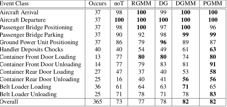
Event Class Occurs noT RGMM DG DGMM PGMM
Aircraft Arrival 37 98 100 99 100 100
Aircraft Departure 37 100 100 100 100 100
Passenger Bridge Positioning 37 98 100 97 100 96
Passenger Bridge Parking 37 90 92 98 99 99
Ground Power Unit Positioning 37 86 79 96 89 87
Handler Deposits Chocks 40 40 54 49 61 63
Container Front Door Loading 13 77 80 80 74 80
Container Front Door Unloading 14 77 79 83 81 91
Container Rear Door Loading 27 47 37 40 53 58
Container Rear Door Unloading 25 16 40 41 56 56
Belt Loader Loading 36 61 64 63 71 65
Belt Loader Unloading 25 71 78 71 78 83
[image:9.408.24.386.30.202.2]Overall 365 73 77 78 82 82
Table 1: Numbers of occurrences of each event class in dataset and Average Precision of detection techniques.
4.2
Training Independent Event Detectors
We refer to results of [20] ,[11] as motivation for using Histograms of Optical Flow (HOF) as the features in our pipeline. Several of our events involve very slow and gradual move-ments, whilst in others objects accelerate rapidly making us wary of employing interest point detection for feature extraction. To handle the variation, it might be possible to tune interest point detectors for each event, but we simply use dense sampling in all cases and rely on our non-linear classifier to distinguish the features which are relevant. Since all events in our vocabulary must happen in designated areas, we are able to specify zones of interest rele-vant to each event and by using local features within these areas get the flexibility of local features whilst eliminating large amounts of noise. The zones used are depicted in Figure3. Similarly, we fix the scale of the features for all event detectors to a block size of 3×3×2, with a cell size of 18×18×8 pixels. We validated our implementation by testing on the KTH actions dataset [17] and recorded results in line with [20].
We perform K-means clustering over 500,000 randomly sampled feature vectors to build a codebook of 4000 spatiotemporal words. Using this codebook, we convert extracted fea-tures to a 4000 dimensional histogram at each timestep in each zone. These vectors are then stacked through time in a matrices of size 4000×T, summing cumulatively over the time dimension. This representation makes it possible to extract the bag of words for any inter-val with just one row subtraction. We train a binary SVM with probabilistic output using libsvm [3], for each event with a χ2 kernel [10] on the ground truth samples and 10,000
negative samples (with mid point sampled randomly and duration sampled from a Gaussian distribution over duration for that event class).
At detection time, we pass histograms corresponding to every possible midpoint and all durations within 2 standard deviations of the mean for each event type to our trained classifiers, and the classifier for each event class supplies the probability of that interval containing an instance of that event.
recall graphs for each event. It was possible to obtain these naturally for the independent detector output by varying a threshold and taking non-overlapping local maxima; and in the case of the temporal models by varying theαcivariables in Equation1.
There are five different sets of results in Table1: ‘noT’ corresponds to the thresholded independent event detector output without a temporal model, ‘DGMM’ is our full model, ‘RGMM’ is the same model but with the tree structure determined randomly, ‘PGMM’ is again the same model but using a fixed tree structure determined in the manner of Pictoral Structure Models [6], ‘DG’ is the case where the pairwise probabilities are modelled by a single Gaussian, but we use our dynamic structure assignment.
Its clear that for almost all events, all variants of our temporal model perform signifi-cantly better than the ‘noT’ detector. Our observation that the single Gaussian was a poor approximation for the pairwise distributions has been validated with the GMM-based models performing better in almost all cases. There are a couple of exceptions to this; on the Con-tainer Front Door Loading/Unloading events the single Gaussian does well. It is likely no coincidence that these are the events with fewest occurrences in the dataset meaning that the pairwise distributions learnt in relation to them would have been trained on just a handful of examples. We put no special mechanism in place to deal with such cases; relying instead on our Bayesian GMM training method to avoid overfitting. The ‘RGMM’ results highlight the need for a good structure learning procedure when applying tree-shaped priors, displaying worse performance even than the ‘DG’ method. There is no clear winner from the other two connection strategies we tested, with both ‘DGMM’ and ‘PGMM’ performing consistently well suggesting that use of the data offered no advantage over a strong offline strategy in this case.
5
Conclusion
GREENALL, COHN, HOGG: TSMS FOR EVENT RECOGNTION
6
Acknowledgments
We thank colleagues in the Co-Friend project consortium (www.cofriend.net) for their valu-able inputs to this research, and the EU Framework 7 for financial support (Co-friend FP7-ICT-214975).
References
[1] Christopher M. Bishop. Pattern Recognition and Machine Learning (Information Science and Statistics). Springer-Verlag New York, Inc., Secaucus, NJ, USA, 2006. ISBN 0387310738. [2] M. Bregonzio, S. Gong, and T. Xiang. Recognising action as clouds of space-time interest points.
In Computer Vision and Pattern Recognition, 2009. CVPR 2009. IEEE Conference on, pages 1948–1955. IEEE, 2009.
[3] C.C. Chang and C.J. Lin. LIBSVM: a library for support vector machines. 2001.
[4] P. Dollar, V. Rabaud, G. Cottrell, and S. Belongie. Behavior recognition via sparse spatio-temporal features. InVisual Surveillance and Performance Evaluation of Tracking and Surveil-lance, 2005. 2nd Joint IEEE International Workshop on, pages 65–72, 2005.
[5] O. Duchenne, I. Laptev, J. Sivic, F. Bach, and J. Ponce. Automatic annotation of human actions in video. InComputer Vision, 2009 IEEE 12th International Conference on, pages 1491–1498. IEEE, 2010.
[6] P.F. Felzenszwalb and D.P. Huttenlocher. Pictorial structures for object recognition.International Journal of Computer Vision, 61(1):55–79, 2005. ISSN 0920-5691.
[7] S. Hongeng, R. Nevatia, and F. Bremond. Video-based event recognition: activity representation and probabilistic recognition methods. Computer Vision and Image Understanding, 96(2):129– 162, 2004.
[8] Yuri A. Ivanov and Aaron F. Bobick. Recognition of visual activities and interactions by stochas-tic parsing. IEEE Transactions on Pattern Analysis and Machine Intelligence, 22(8):852–872, 2000. ISSN 0162-8828. doi: http://doi.ieeecomputersociety.org/10.1109/34.868686.
[9] J.B. Kruskal. On the shortest spanning subtree of a graph and the traveling salesman problem.
Proceedings of the American Mathematical society, 7(1):48–50, 1956.
[10] I. Laptev, B. Caputo, C. Schüldt, and T. Lindeberg. Local velocity-adapted motion events for spatio-temporal recognition.Computer Vision and Image Understanding, 108(3):207–229, 2007. [11] I. Laptev, M. Marszalek, C. Schmid, and B. Rozenfeld. Learning realistic human actions from movies. InIEEE Conference on Computer Vision and Pattern Recognition, 2008. CVPR 2008, pages 1–8, 2008.
[12] P. Matikainen, M. Hebert, and R. Sukthankar. Representing pairwise spatial and temporal rela-tions for action recognition. Computer Vision–ECCV 2010, pages 508–521, 2010.
[13] J.C. Niebles, H. Wang, and L. Fei-Fei. Unsupervised learning of human action categories using spatial-temporal words.International Journal of Computer Vision, 79(3):299–318, 2008. [14] Juan Carlos Niebles, Chih-Wei Chen, , and Li Fei-Fei. Modeling temporal structure of
Transactions on Pattern Analysis and Machine Intelligence, 22(8):747–757, 2000.
[19] V.T. Vu, F. Brémond, and M. Thonnat. Automatic video interpretation: A novel algorithm for temporal scenario recognition. InProceedings of the 18th international joint conference on Arti-ficial intelligence, pages 1295–1300. Morgan Kaufmann Publishers Inc., 2003.
[20] H. Wang, M.M. Ullah, A. Klaser, I. Laptev, and C. Schmid. Evaluation of local spatio-temporal features for action recognition. InBritish Machine Vision Conference, London, UK, pages 1–11, 2009.