Developing measures for valuing changes in biodiversity:
Final Report
Report to
DEFRA
London
From
Dr Mike Christie1, Dr John Warren1, Prof. Nick Hanley2, Dr. Kevin Murphy2, Prof. Robert Wright3, Mr Tony Hyde4 and Mr Nick Lyons4
1University of Wales Aberystwyth 2University of Glasgow
3University of Stirling 4 Socio-Economic Research Services
Table of contents
DEVELOPING MEASURES FOR VALUING CHANGES IN BIODIVERSITY: ... 1
TABLE OF CONTENTS... 2
LIST OF TABLES... 5
LIST OF FIGURES... 5
EXECUTIVE SUMMARY ... 6
1. INTRODUCTION ... 11
1.1. WHY VALUE BIODIVERSITY?... 11
1.2. VALUING BIODIVERSITY: THE CHALLENGE! ... 12
1.3. STRUCTURE OF REPORT... 13
2. AN ECOLOGIST’S PERSPECTIVE OF BIODIVERSITY ... 14
2.1. DEFINING BIODIVERSITY... 14
2.2. MEASURING BIODIVERSITY... 15
2.2.1. Is biodiversity just the number of species in an area?... 15
2.2.2. If biodiversity is more than the number of species how can it be measured?... 17
2.2.3. Are all species of equal weight?... 18
2.2.4. Should biodiversity measures include intraspecific genetic variability? ... 21
2.2.5. Do certain species contribute more than others to the biodiversity of an area?... 21
2.2.6. Are there useful indicators of areas where biodiversity is high? ... 24
2.2.7. Can the extent of biodiversity in taxonomic groups be estimated by extrapolation? ... 24
2.2.8. Can biodiversity be used as a measure, or indicator, of the health of ecosystems?... 25
2.3. THE UK BIODIVERSITY RESOURCE... 28
2.4. IS BIODIVERSITY A USEFUL MEASURE FOR ENVIRONMENTAL VALUATION PURPOSES? ... 29
3. AN ECONOMISTS PERCEPTION OF BIODIVERSITY... 31
3.1. CONCEPTS OF ECONOMIC VALUE OF BIODIVERSITY... 31
3.1.1. Direct use values of biodiversity ... 31
3.1.2. Indirect use values of biodiversity ... 32
3.1.3. Other biodiversity value considerations... 32
3.2. METHODS OF ESTIMATING THE ECONOMIC VALUE OF BIODIVERSITY... 33
3.2.1. Direct effects on utility ... 34
3.2.2. Indirect impacts on utility... 36
3.3. REVIEW OF STUDIES THAT AIM TO VALUE OF BIODIVERSITY. ... 36
3.3.1. Review of studies that value the biological resource... 36
3.3.2. Review of studies that value biological diversity... 39
3.4. BENEFITS TRANSFER AND BIODIVERSITY. ... 40
4. IDENTIFICATION OF SUITABLE APPROACHES TO VALUE CHANGES IN BIODIVERSITY... 42
4.1. WHAT ASPECTS OF BIODIVERSITY CHANGE ARE OF MOST INTEREST TO THIS RESEARCH... 42
4.2. HOW DO WE MEASURE BIODIVERSITY CHANGE IN A WAY THAT IS MEANINGFUL TO THE PUBLIC? 42 4.2.1. Development of a conceptual framework in which to present biodiversity. ... 43
4.3. WHICH METHODOLOGY IS LIKELY TO BE MOST SUITED TO THE VALUATION OF THIS CHANGE? 47 4.3.1. Methodology: Suitability Matrix Scoring System (SMSS) for the valuation of biodiversity. ... 48
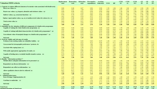
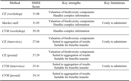
4.3.2. Results from the valuation SMSS... 50
4.4. CONCLUSIONS FROM THE SMSS EXERCISE... 53
4.5. WHAT CAN WE CONCLUDE ABOUT THE SUITABILITY OF ALTERNATIVE METHODS TO VALUING BIODIVERSITY CHANGE? ... 55
5. RESEARCH AIMS AND OBJECTIVES ... 56
5.1. VALUATION OF THE ATTRIBUTES OF BIOLOGICAL DIVERSITY... 56
5.3. EXAMINATION OF BENEFITS TRANSFER OF BIODIVERSITY VALUES... 57
5.4. DEALING WITH THE INFORMATION PROBLEM... 57
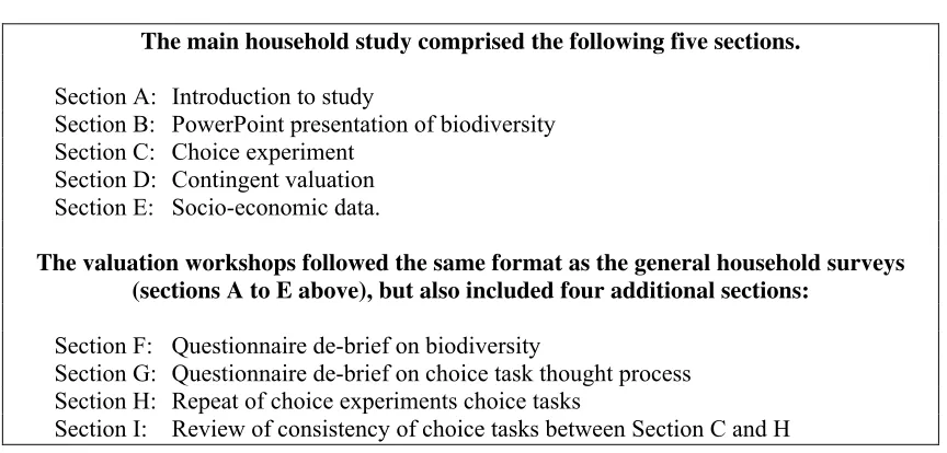
6. RESEARCH METHODOLOGY ... 58
6.1. SECTION A:INTRODUCTION TO STUDY. ... 59
6.2. SECTION B:POWERPOINT PRESENTATION OF BIODIVERSITY... 59
6.2.1. Why MS PowerPoint was used to present biodiversity. ... 59
6.2.2. Content of PowerPoint Presentation... 60
6.3. SECTION D:THE CHOICE EXPERIMENT STUDY... 62
6.3.1. Implementation of the choice experiment... 62
6.3.2. Biodiversity attributes used in the choice experiment ... 63
6.3.3. Design of choice tasks ... 69
6.4. SECTION D:THE CONTINGENT VALUATION STUDY... 69
6.4.1. CV scenario 1: Agri-environmental scheme... 69
6.4.2. CV scenario 2: Habitat re-creation... 70
6.4.3. CV scenario 3: Loss of biodiversity due to development... 71
6.4.4. The CV elicitation question ... 71
6.5. SECTION E:SOCIO-ECONOMIC DATA... 73
6.6. SECTION F:QUESTIONNAIRE DEBRIEF ON LEVEL OF UNDERSTANDING OF BIODIVERSITY CONCEPTS... 73
6.7. SECTION G:REFLECTION ON THE CHOICE TASK... 74
6.8. SECTION H:REPEAT OF CHOICE EXPERIMENTS CHOICE TASKS... 75
6.9. SECTION I:REVIEW OF CONSISTENCY OF CHOICE TASKS BETWEEN SECTION C AND H ... 75
6.10. ADMINISTRATION OF SURVEY... 75
6.10.1. Administration of household survey ... 75
6.10.2. Administration of the valuation workshops ... 76
6.11. TESTS FOR BENEFITS TRANSFER... 76
6.12. DESCRIPTION OF CASE STUDIES... 76
6.12.1. Biodiversity in Cambridgeshire... 76
6.12.2. Biodiversity in Northumberland ... 77
7. RESULTS ... 78
7.1. ANALYSIS OF THE MAIN HOUSEHOLD CONTINGENT VALUATION STUDY... 78
7.1.1. Comparison of CV mean WTP results across case study locations – household interviews 79 7.1.2. Comparison of mean WTP results across policy scenarios... 88
7.1.3. Comparison of CV data from the household study and valuation workshops ... 90
7.2. CHOICE EXPERIMENT RESULTS... 95
7.2.1. Choice experiment results ... 96
7.2.2. Implicit prices for biodiversity attributes ... 98
7.3. VALUATION WORKSHOP RESULTS... 99
7.3.1. Analysis of participants understanding of biodiversity concepts ... 100
7.3.2. Analysis of how participants made their choices in the choice experiment... 101
7.3.3. Choice experiment: comparison of main study and valuation workshop ... 103
8. DISCUSSION... 105
8.1. DO MEMBERS OF THE PUBLIC VALUE PROTECTION AND ENHANCEMENT OF BIODIVERSITY?. 105 8.1.1. Evidence from the CV study to support the thesis that the public do value biodiversity. 105 8.1.2. Are choice experiment respondents willing to pay anything towards biodiversity enhancement scenarios? ... 107
8.2. WHAT ASPECTS OF BIODIVERSITY DO THE PUBLIC VALUE THE MOST?... 109
8.2.1. The value of biodiversity policies ... 109
8.2.2. The value of biodiversity attributes. ... 110
8.3. HOW ROBUST ARE OUR VALUE ESTIMATES?... 112
8.3.1. Validity tests ... 112
8.3.2. Critique of methodologies used ... 114
8.4. CAN OUR BENEFIT ESTIMATES BE TRANSFERRED TO OTHER SITUATIONS?... 116
8.4.1. Tests for benefits transfer from the CV data... 116
8.4.3. Benefits transfer implication ... 118
9. CONCLUSIONS ... 119
9.1. MEASUREMENT OF THE ECONOMIC VALUE OF POLICY PROGRAMMES WHICH ENHANCE AND PROTECT BIODIVERSITY. ... 119 9.2. MEASUREMENT OF THE ECONOMIC VALUE OF THE COMPONENT ATTRIBUTES OF BIOLOGICAL DIVERSITY... 120
10. REFERENCES ... 124
List of Tables
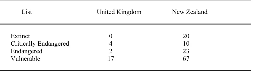
Table 1: IUCN red-data listed terrestrial species... 29
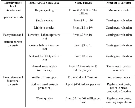
Table 2: Value ranges for biological resources ... 38
Table 3: Scoring criteria used in the Valuation SMSS ... 49
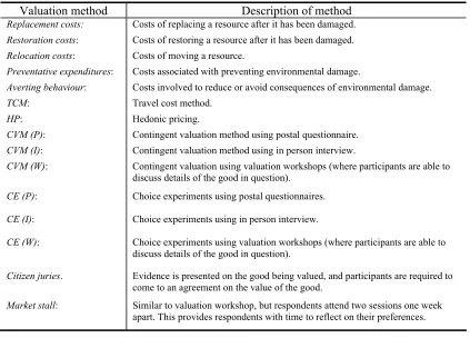
Table 4: Valuation methods assessed in the Valuation SMSS ... 50
Table 5: Results from the SMSS ... 51
Table 6: Summary of strengths and limitations of alternative valuation methods ... 54
Table 7: Summary of biodiversity attributes and levels used in the choice experiment ... 64
Table 8: Summary WTP Measures for any policy improvement scenario... 79
Table 9: Summary WTP Measures - Habitat Re-creation Only ... 80
Table 10: Summary WTP Measures: Development Loss Only... 80
Table 11: WTP Equations - Cambridgeshire and Northumberland... 82
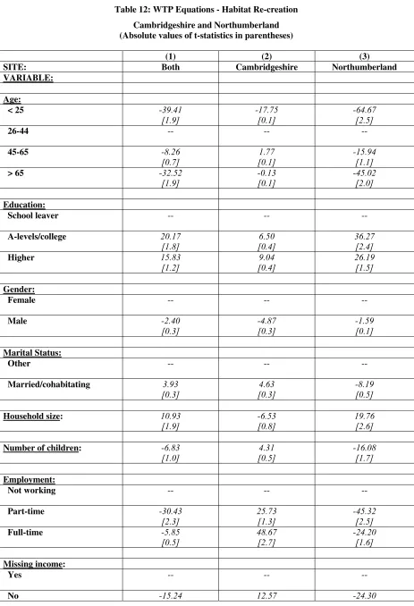
Table 12: WTP Equations - Habitat Re-creation... 84
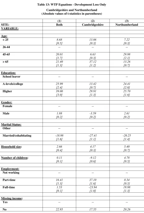
Table 13: WTP Equations - Development Loss Only ... 86
Table 14: Summary WTP Measures by Type of Policy scenario (Cambridgeshire Only)... 88
Table 15: Summary WTP Measures by Type of Policy scenario (Northumberland Only)... 88
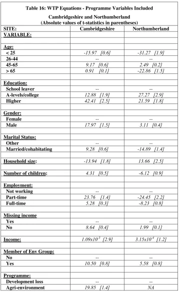
Table 16: WTP Equations - Programme Variables Included ... 89
Table 17: Summary WTP Measures for ‘pooled’ policy scenarios: Valuation Workshop versus Main Survey (Northumberland Only) ... 90
Table 18: Summary WTP Measures for Habitat Re-creation scenario: Valuation Workshop versus Main Survey (Northumberland Only) ... 91
Table 19: Summary WTP Measures for Development Loss scenario: Valuation Workshop versus Main Survey (Northumberland Only) ... 91
Table 20: Summary WTP Measures: Valuation Workshop Only (Northumberland Only) .... 92
Table 21: WTP Equations - Valuation Workshop and Main Survey ... 93
Table 22: Logit models for Cambridge and Northumberland CE samples ... 97
Table 23: Implicit prices for Cambridge and Northumberland CE samples ... 99
Table 24: Analysis of level of understanding of biodiversity (Before and After discussion) 100 Table 25: Choice making strategy: level of consideration of choice experiment attributes.. 101
Table 26: Choice making strategy: level of consideration of the ‘price’ attribute. ... 102
Table 27: Choice making strategy: level of consideration of level of the ‘price’ attribute. .. 102
Table 28: Choice experiment results: workshop versus main survey, Northumberland ... 104
Table 29: Proportion of household CV respondents stating that they would be willing to pay towards biodiversity. ... 106
Table 30: Stated reasons why CV respondents were WTP towards biodiversity scenarios.. 106
Table 31: Stated reasons why CV respondents were NOT WTP towards biodiversity scenarios ... 107
Table 32: Proportion of household CE respondents choosing the alternative biodiversity options ... 108
Table 33: Stated reasons for making CE choices. ... 108
Table 34: Workshop participant's perceptions of scope of biodiversity policies ... 115
List of Figures
Figure 1: Conceptual framework – Measures of biodiversity ... 44Figure 2: Conceptual framework – Biodiversity concepts ... 44
Executive summary
This document reports the findings from the DEFRA funded research project ‘Developing measures for valuing changes in biodiversity’. The aim of the research was to develop an appropriate framework that will enable cost-effective and robust valuations of the total economic value of changes to biodiversity in the UK countryside. The research involved a review of ecological and economic literature on the valuation of biodiversity changes. The information gathered from this review, along with the findings from a series of public focus groups and an expert review of valuation methodologies, were used to develop a suite of valuation instruments that were used to measure the economic value of different aspects of biodiversity. Contingent valuation and choice experiment studies were administered to households in Cambridgeshire and Northumberland, while valuation workshops were conducted in Northumberland only. The data from these studies were also used to test for benefits transfer.
Review of ecological and economic literature
The key issues identified in the review of ecological literature included: • There is no one simple measure of biodiversity.
• Ecologists agree that species richness (the number of species per unit area) is a useful starting point for measuring biodiversity. However, there are issues regarding definitions of species and identification of a suitable area in which to measure biodiversity.
• Ecologists also recognise that some species are likely to be more important than other species with respect to enhancing and conserving biodiversity, e.g. keystone species and umbrella species.
• It was also recognised that humans may have anthropocentric preferences for certain species (e.g. cute and charismatic species), even though these species may not necessarily be important in ecological / biodiversity terms.
• Biodiversity may also be measured in terms of habitat diversity and ecosystem diversity.
The economic review highlighted the following issues:
• The total economic value of biodiversity comprises direct values (use, passive-use and options values) and indirect values.
• There are a range of methodologies available to value biodiversity change including revealed preference, stated preference, and cost-based approaches. However, no one method was considered to be capable of valuing all aspects of TEV associated with biodiversity change.
• Revealed preference methods (e.g. travel cost method and hedonic pricing) are largely restricted to the measurement of use values.
• Stated preference methods (e.g. contingent valuation and choice experiments methods) are in theory capable of estimating both use and passive-use values. However, in practice they are less suited to measuring indirect issues such as ecosystem services. The choice experiments approach has the added advantage that it is also capable of valuing the component elements of biodiversity.
• Cost-based approaches (e.g. replacement costs, restoration costs, preventative expenditures) infer a value for natural resources (including ecosystem functions and services) by how much it costs to replace or restore a resource after it has been damaged. In other words, these techniques do not measure the utility or economic value accrued to individuals from improvements in biodiversity.
particular the value of individual species and habitats), few studies have attempted to value biological diversity per se. Furthermore, very little research has attempted to disentangle the value of the components of biodiversity.
Methodology and results
A series of developmental focus groups were undertaken to explore public understanding of the biodiversity concepts identified in the review to ecological and economic literature. The key findings from the focus group were that public understanding of the term biodiversity is generally low. However, the public do have the capacity to understand the concepts of biodiversity if described in layman’s terms. Furthermore, it was clear that the way in which the public consider biodiversity is different to the way in which ecological experts consider biodiversity. Thus an important lesson from this is that studies that value complex goods such as biodiversity need to be careful in the way they present information on that good.
The actual valuation study utilised three survey instruments: a contingent valuation study, a choice experiment study and a series of valuation workshops. The contingent valuation and choice experiment studies were combined into a single survey instrument, which was administered to 400 household in both Cambridgeshire and Northumberland. During these interviews, information on biodiversity was presented using an innovative MS PowerPoint presentation. Six valuation workshops were administered in Northumberland only. The format of the workshops initially followed that of the household surveys, but also included further discussion of biodiversity and the choice task, as well as a further series of choice experiment choice tasks.
Contingent valuation study
The contingent valuation study addressed three biodiversity enhancing and protection policies:
• An agri-environmental scheme that aimed to enhance biodiversity on arable land through the creation of conservation headlands and the reduced application of pesticides and herbicides. Biodiversity benefits from this scheme would include an increased diversity of plants, insects, small mammals and birds; some of which may be rare.
• A habitat re-creation scheme that would enhance biodiversity by creating new wetland habitats on existing farmland. The new wetland would provide habitats for a wide range of plants, insects, small mammals and birds, including a number of rare species. In addition, the wetland area would provide ecosystem services such as flood protection and enhanced water quality.
• The third scheme would aim to avoid biodiversity loss as a result of housing development on farmland managed under existing agri-environmental schemes. The types of biodiversity protected under this policy would be similar to those described in the agri-environmental scheme above.
The key findings from the contingent valuation study included:
• In Cambridgeshire, the value of the agri-environmental, habitat re-creation and protect against biodiversity loss from development policies were £74.27, £54.97 and £45.30 respectively, where these values related to annual WTP amounts per household over a five year period.
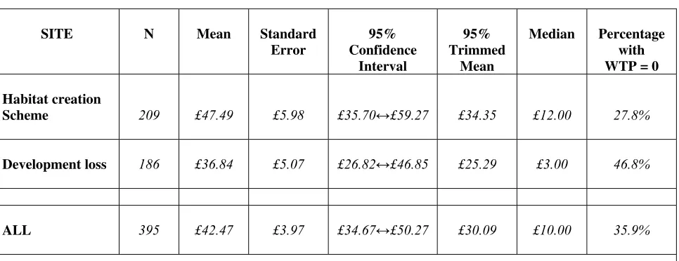
• In Northumberland, the values of the habitat re-creation scheme and protect against biodiversity loss from development schemes were £47.49 annually per household and £36.84 annually per household respectively.
• Furthermore, the estimated WTP values for the alternative policy scenarios were not found to be statistically different from one another.
• There was some evidence of consistency in mean WTP values for policies between the two case study areas, however, this was not the case for the transfer of the bid functions.
• The key policy implications of the above findings are that the public are willing to pay a positive sum of money for biodiversity enhancing and protecting policies. However, there were no significant differences between the values of the alternative policy prescriptions. Thus, we are unable to make clear recommendations with regard to which types of biodiversity policy should take priority.
Choice experiment method
The second method utilised was the choice experiment method. The CE study assessed the value of four attributes of biodiversity:
• Familiar species of wildlife. This attribute was described to include the concepts of charismatic, familiar (recognisable) and locally symbolic species. Three levels of this attribute were presented: protection of rare familiar species, protection of rare and common familiar species, and the status quo (continued decline).
• Rare, unfamiliar species of wildlife. This attribute focused on those species that are currently rare or in decline which are unlikely to be familiar to members of the public. The three levels of this attributes included: the slow down of decline of rare unfamiliar species, the recovery of populations of rare unfamiliar species and the status quo (continued decline).
• Species interactions within a habitat. This attribute was used to represent the importance of species interactions within a habitat, as well as a proxy for the preservation of ecologically significant species such as keystone and umbrella species. Levels of provision of this attribute included: habitat restoration, habitat re-creation and the status quo (continued decline).
• Ecosystem processes. Ecosystem processes focused on biodiversity’s role in preserving the health of ecosystem processes. Levels of this attribute included: preservation of ecosystem processes that directly affect humans, preservation of all ecosystem processes, and the status quo (continued decline).
The key findings from the CE study were as follows:
• The attribute that targeted the ‘recovery of rare unfamiliar species’ attained the highest implicit price (£115 and £189 respectively for Cambridgeshire and Northumberland). Furthermore, this attribute was the only one that was valued significantly higher than any of the other attributes.
• In contrast to the above, the ‘slow down the rate of decline of rare unfamiliar species’ was found to be negative in the Cambridgeshire sample, while the attribute level was not significant in the Northumberland CE model.
• In Northumberland, both the protection of ‘rare familiar species’ (£90.59) and ‘both rare and common familiar species’ (£97.71) were found to achieve consistently high implicit prices, while in Cambridgeshire the protection of ‘rare familiar species’ (£35.65) was found to be significantly lower than the protection of ‘rare and common familiar species’ (£93.49).
• In Northumberland, the ‘habitat restoration’ attribute (£71.15) was found to be similar to the ‘habitat re-creation’ attribute (£74.00), while in Cambridgeshire the ‘habitat re-creation’ attribute (£61.36) achieve a higher implicit price than the ‘habitat restoration’ attribute (£34.40).
human impact level) was not significant in Northumberland and was lower than the human impact level in Cambridgeshire. The reason for this findings appears to stem from the fact that generally there was a lower level of understanding of this attribute and therefore people valued it less.
The key policy implications of the CE data is that the public do value most, but not all, biodiversity attributes and that they appear to be able to distinguish between alternative attributes (but perhaps not always attribute levels). In particular, there is evidence to support the continued funding of policies that target species, habitats and ecosystem processes. Of particular interest is the finding that the public have high values for the protection of rare unfamiliar species; thus policies should not be restricted to target only familiar and charismatic species. Second, the comparison of the results between Cambridgeshire and Northumberland for the rare familiar species attribute level and the habitat restoration attribute level are interesting in that it would appear that people in Cambridgeshire have low values for these two attribute levels as a direct result of the perception that Cambridgeshire currently does not support such biodiversity.
Valuation workshop
Six valuation workshops (53 participants) were administered in Northumberland. The format of the workshops followed that of the household surveys, but also included further opportunities to discuss biodiversity and five further choice experiment tasks. The key findings from the workshops included:
• The information presented in the PowerPoint presentation allowed participants to attain a good understanding of all biodiversity attributes apart from the ecosystem processes attribute.
• Although the extra discussions in the workshop improved participants understanding of biodiversity concepts, this extra level of knowledge did not significantly influence their values for the biodiversity attributes.
• The discussion of the participant’s choice strategies provided evidence that participants were using consistent and consider valuation choices.
Conclusions
We argue that this research has been successful in attaining meaningful and robust values for complex goods. Evidence supporting this claim comes from a number of sources including the validity tests for the alternative valuation studies and the responses from the valuation workshop. We, however, stress that valuing complex goods is challenging, and in particular a lot of effort needs to be undertaken in developing the hypothetical descriptions of the goods in question. In our study, this effort included an ‘expert’ (ecologists) review of biodiversity and a series of focus groups to ‘translate’ the expert view into a language which was both understandable and meaningful to the public. Also we presented the information using an innovative MS PowerPoint presentation.
1. Introduction
This document reports the research undertaken for a DEFRA funded project ‘Developing measures for valuing changes in biodiversity’. The aim of the research contract is ‘to develop an appropriate framework that will enable cost-effective and robust valuations of the total economic value of changes to biodiversity in the UK countryside’.
Before getting into the detail of this report, it is first useful to provide some background on why one might be interested in measuring the economic value of biodiversity and second to identify some of the potential problems and challenges that researchers may encountered while undertaking such a valuation exercise.
1.1. Why value biodiversity?
Biodiversity is important to humans for various reasons. First, biodiversity may increase an individual’s welfare directly. This may be through actual use of a biological resource (e.g. recreational use of natural areas) or through passive-use benefits (e.g. derived from the knowledge that biodiversity is being protected for future generations to enjoy). Biodiversity may also increase an individual’s welfare indirectly through its contribution towards the maintenance of ecosystem functions such as the regulation of the water and carbon cycles (Fromm, 2000; Pimm et al., 1995). The conservation of the Earth’s biological resources is thus essential to preserve the well-being of both current and future generations.
Human activities, however, have also contributed towards the unprecedented decline in the Earth’s biodiversity. This, in turn, may be threatening the stability of the Earth’s ecosystem functions, as well as the capacity of the Earth to provide ecosystem services to man. In order to protect and maintain the Earth’s biodiversity, human society needs to make difficult decisions regarding its use of biological resources. For example, policies may need to be adopted to reduce livestock stocking densities on farmland to promote biodiversity. Environmental valuation techniques can provide useful evidence to support such policies by quantifying the economic value associated with the protection of the Earth’s biological resource. Pearce (2001) argues that the measurement of the economic value of biodiversity is a fundamental step in conserving the biological resource since ‘the pressures to reduce biodiversity are so large that the chances that we will introduce incentives [for the protection of biodiversity] without demonstrating the economic value of biodiversity are much less than if we do engage in valuation’. Assigning monetary values to biodiversity is thus important since it allows the benefits associated with biodiversity to be directly compared with the economic value of alternative resource use options. Such evidence is likely to greatly to assist in the formulation of policies that protect biodiversity. OECD (2001) also recognises the importance of measuring the economic value of biodiversity and identifies a wide range of uses for such values, including:
• Demonstrating the value of biodiversity: awareness raising showing the importance of biodiversity,
• Determining damages for loss of biodiversity: liability regimes, • Revising the national economic accounts,
• Setting charges, taxes, fines,
• Land use decisions, e.g. to make a case for sustainable agriculture / forestry or to protect an area,
• Limiting biological invasions,
• Limiting or banning trade in an endangered species,
Furthermore, it is evident that the role of environmental valuation methodologies in policy formulation is increasingly being recognised by policy makers. For example, the Convention of Biological Diversity’s Conference of the Parties decision IV/10 acknowledges that ‘economic valuation of biodiversity and biological resources is an important tool for well-targeted and calibrated economic incentive measures’ and encourages Parties, Governments and relevant organisations to ‘take into account economic, social, cultural and ethical valuation in the development of relevant incentive measures’. The EC Environmental Integration Manual (2000) provides guidance on the theory and application of environmental economic valuation for measuring impacts to the environment for decision-making purposes. The manual suggests that environmental valuation should be undertaken alongside Environmental Assessment studies. Within the UK, the HM Treasury’s ‘Green Book’ provides guidance for public sector bodies on how to incorporate non-market costs and benefits into policy evaluations.
1.2. Valuing biodiversity: the challenge!
Although environmental valuation techniques are increasingly being utilised to aid policy formulation, there is however still some latent resistance to placing monetary values on biodiversity. In particular, some environmental analysts argue that nature has non-anthropocentric “intrinsic values” and thus non-human species possess moral interests or rights (O’Neil, 1997; Ehrenfeld, 1988). Such positions lead to the advocacy of environmental sustainability standards, which to some extent preclude the need for valuation. However, general consensus accepts that placing monetary values on biological resources makes explicit the fact that biodiversity is used for instrumental purposes in terms of productive and consumptive opportunities (Fromm, 2000; Nunes and van den Bergh, 2001) and therefore will help policy makers make more informed decisions regarding the use of biological resources. The validity of the various valuation methodologies have also been questioned (Bate, 1993) and as a consequence many of these methods have been subject to intensive academic debate and scrutiny. One of the key assessments of the validity of stated preference valuation methods (and the contingent valuation (CV) method in particular) occurred in 1993 following a natural resource damage assessment of the Exxon Valdez Oil disaster off the coast of Alaska. As part of the damage assessment, a contingent valuation study was conducted to assess the passive-use values associated with the prevention of future oil spills. The results from this study sparked an intensive debate on the validity of CV. To resolve this debate, a NOAA (National Oceanic and Atmospheric Administration) blue ribbon panel of experts was set up to review the validity of CV. The conclusions from this review was ‘that CV studies can produce estimates reliable enough to be the starting point of a judicial process of damage assessment, including lost passive use values’ (Arrow et al., 1993). However, the NOAA panel recognised that there was a variability in the quality of CV studies and therefore produced a set of guidelines for CV.
In addition to concerns regarding the validity of valuation methods, there are also a number of concerns relating to the valuation of biodiversity that need to be considered. These include incommensurate values, lexicographic preference issues (Spash and Hanley, 1995; Spash, 1993), the problem of dealing with protest votes (Spash, 1993), intergenerational rights issues (Bromley, 1995), people’s understanding of a complex good (Christie, 2001; Limburg et al., 2002).
the problem. Studies have consistently found that members of the general public have a low awareness and poor understanding of the term biodiversity. For example, quantitative research undertaken in 1988 found that 63% of a UK sample did not know what the words ‘biological diversity’ meant (MORI, 1988b). More recent work for the Scottish Office confirms that public understanding of environmental terminology, including ‘biodiversity’, is very low. However, a study valuing biodiversity in British forests reported that although respondents generally had a poor understanding of the importance of wildlife in itself, ‘environmentalists’ and ‘outdoor enthusiasts’ were found to have a clearer understanding of ecological systems (ERM, 1996). This was also the case in a study valuing endangered species (Macmillan et al., 2001b) where responses demonstrated an understanding of the environment in general and more specifically wildlife conservation. Furthermore, other studies found that the UK public disliked the phrase ‘biological diversity’, preferring the terms ‘variety of life’, ‘living diversity’ and ‘biological variety’ (MORI, 1988a), or ‘variety of wildlife’ (ERM, 1996). Other research has shown that once the concept of biodiversity was explained in layman’s term a high proportion of the general public (78%) considered that ‘biological diversity’ was important (MORI, 1991). The findings from these studies will have significant implications for the valuation of biodiversity. In particular, the lack of public understanding of the term biodiversity will make the valuation exercise extremely difficult. The issues highlighted above indicate that research that attempts to value changes in biodiversity will be challenging. Not only will research need to address and overcoming many methodological issues associated with environmental valuation techniques, but it will also need to identify appropriate language in which biodiversity concepts can be meaningfully conveyed to members of the public, thus enabling them to express their preferences. The research described in this report aims to address these challenges.
1.3. Structure of report
2. An Ecologist’s Perspective of Biodiversity
2.1. Defining biodiversity
The concept of biological diversity, originally simply meaning “number of species present”, appears to have been first developed in the sense in which it is used today during the 1970s – early 1980s (Peet, 1974; Lovejoy, 1980a,b; Norse & McManus, 1980), despite attempts to strangle the idea at birth (Hurlbert, 1971). A few years later, Norse et al. (1986) defined biological diversity at the genetic (within-species), species (species numbers), and ecological (community) level. The contracted term “biodiversity” came from a “National Forum on Biodiversity” held in the USA in 1986, the Proceedings of which (Wilson, 1988) brought the term, and concept, into more general use.
Although there are many possible definitions, perhaps the most widely-accepted is that provided in Article 2 of the “Convention on Biological Diversity” (signed by 157 national and supra-national organizations) at the 1992 UN Conference on the Environment and Development:
“Biological diversity” means the variability among living organisms from all sources, including, inter alia, terrestrial, marine and other aquatic systems and the ecological complexes of which they are part; this includes diversity within species, between species and of ecosystems.
More recently, Harper & Hawksworth (1995), in the preface to The Royal Society’s review of the biological diversity concept, suggested that biodiversity is best considered at three levels, ‘genetic’, ‘organismal’, and ‘ecological’ (or ‘community’) biodiversity. There is general agreement today that this approach is appropriate in the study of biodiversity - environment relationships. Current major ecological research effort, worldwide, is focused on understanding the implications of biodiversity for ecosystem productivity and functioning (e.g. Aarssen, 1997; Diemer et al., 1997; Hodgson et al., 1998; Yachi & Loreau, 1999; Hughes & Roughgarden, 2000; Cottingham et al., 2001); and also in assessing human impacts on biodiversity, and the ecosystems which support biological communities (e.g. Willoughby, 1992; Chapin et al., 1998; Naeem et al., 1995; Sala et al., 2000).
For example, in the context of environmental-related human impacts (in this case acidification, eutrophication, potential CO2 increase, and leisure-use increase) upon the aquatic plant biodiversity of European lake ecosystems, Murphy (2003) suggested that diversity responses at these three scales were an appropriate basis for assessment:
• Genetic level diversity. Genetic variation may be partitioned within or between populations and may be the basis of locally adapted populations, races, and sub-species. It may be quantified at the molecular level, although historically such variation was described based on the measurement of physiological or morphological traits (e.g. Pieterse et al., 1984; Nielsen and Sand-Jensen, 1997; Vöge, 1997a,b; Madeira et al., 1999; Hollingsworth et al., 1995, 1996).
• Functional / ecological diversity. This is a more complex concept (Steneck & Dethier, 1994; Hills et al., 1994; Herrera et al., 1997). It relates to the complexity of ecosystems processes (number of interactions) occurring within a community, which arise from the number of functional groups of organisms present (Farmer and Spence, 1986; Murphy et al., 1990).
In addition to assessing what is meant by the term “biodiversity”, Harper & Hawksworth (1995) also identified seven major questions related to measuring biodiversity, some of which have been addressed reasonably well at the present time, while others still require considerable research to answer properly.
The questions are summarized below:
1. Is biodiversity just the number of species in an area?
2. If biodiversity is more than the number of species, how can it be measured? 3. Are all species of equal weight?
4. Should biodiversity measures include intraspecific genetic variability? 5. Do certain species contribute more than others to the biodiversity of an area? 6. Are there useful indicators of areas where biodiversity is high?
7. Can the extent of biodiversity in taxonomic groups be estimated by extrapolation?
To this set we may add two additional questions, relevant to the issue of predicting change in biodiversity, and using such change to assess the value and health of ecosystems:
8. Can biodiversity be used as a measure, or indicator, of the health (“biointegrity”) of ecosystems?
9. Is biodiversity a useful measure for environmental valuation purposes?
The above nine questions have been identified by ecologists as a useful approach to the definition and measurement of biodiversity changes. We now explore each of these questions in turn, highlighting how ecological concepts may be translated to form the foundation of the valuation exercise.
2.2. Measuring biodiversity
2.2.1. Is biodiversity just the number of species in an area?
Biodiversity is frequently divided into a hierarchy of three levels: ecosystems/habitats, species and genes. Ecosystems are defined as communities of co-occurring species of plants and animals plus the physical environment; as such they are difficult to define and delimit. At the other end of the spectrum, genes are currently still difficult to identify and count. Thus, species counting is the obvious tool for measuring biodiversity. Therefore, although biodiversity may be measured at levels from genome to biome (Colwell and Coddington, 1994; Roy and Foote, 1997; Hawksworth, 1995; Lovejoy 1995; Magurran 1988), measurement of the number of species present (S) within a defined target area is generally accepted as one of the simplest measures of biodiversity. This of course raises the problem of defining the target area in which to record the inventory of species, which again requires the ability to define and delimit ecosystems. Whittaker (1977) identified four levels at which it is useful to measure species diversity. The smallest of these scales is point diversity, or micro-habitat diversity in which the inventory area is defined as being a homogeneous micro-habitat. Above this level is alpha diversity or within-habitat diversity, which is probably the most widely used scale for recording species numbers. The third scale of diversity, gamma
different ecosystems within a local area, and may include areas such as islands. The largest scale is Whittaker’s fourth-level; epsilon or regional diversity, which applies to large biogeographic area, and comprises the total diversity of a group of areas of gamma diversity. To be able to compare areas in terms of their diversity Whittaker coined three additional levels of differentiation diversity (pattern diversity, beta diversity and delta diversity).
Pattern diversity is defined as the measure of differentiation diversity between samples taken within a homogeneous habitat. Beta diversity (or between habitat diversity) is by far the most widely used measure of differentiation diversity. It is defined as the change in species composition and abundance between areas of gamma diversity. Beta diversity can be estimated as change in species diversity along a gradient (Wilson & Mohler, 1983) or by comparing the species composition of different communities. Delta diversity is defined as the change in species composition and abundance between areas of gamma diversity, which occur within areas of epsilon diversity. As such it is used to represent differences in diversity over wide biogeographic areas. In addition to these four levels of species diversity, and three levels of differentiation diversity, ecologists also measure diversity in terms of the structural complexity of habitats and how it relates to niche width.
Once the area to be considered has been defined, Harper & Hawksworth (1995) identified a further problem in basing biodiversity measures on a simple taxonomic concept. They postulated a site of defined area, containing just two organisms (i.e. S = 2), one being a plant species of the genus Ranunculus (e.g. Ranunculus acris: meadow buttercup), and the other from a list including:
a. another species of Ranunculus from the same section of the genus (e.g. Ranunculus repens: creeping buttercup),
b. another species of Ranunculus from a different section of the genus (e.g. Ranunculus ficaria: lesser celandine),
c. a species from a different genus in the family Ranunculaceae (e.g. Anemone nemorosa: wood anemone),
d. a species from a different plant family, in a different order (e.g. a grass such as
Anthoxanthum odoratum: sweet vernal grass), e. a fungus of the genus Agaricus,
f. a rabbit.
In taxonomic terms the diversity within the site is generally increasing as we go down this list because the species involved are further apart in evolutionary terms. As Harper & Hawksworth (1995) point out “…any measure of biodiversity which described all these sites as equal would be particularly uninformative”: as is clearly shown by the fact that the measure remains at S = 2 throughout this series.
The answer to this problem lies in clearly identifying the basis for comparison of S (e.g. between sites, or over time, or both) on a taxonomic basis (e.g. for specified plant groups down to species level only: Wilson et al., 2003; for birds: Parish et al., 1994); or on a functional basis (e.g. McGrady-Steed & Morin, 2000; Symstad et al., 2000). Where “like with like” comparisons of change in S can be made, in this way, then potentially useful trends and changes in biodiversity can be identified which are of practical use for policy, conservation, or management purposes.
In practical terms, probably the majority of recent studies which have aimed at examining and/or predicting biodiversity change, in relation to human activities, have incorporated S as (at least one) indicator of biodiversity status. Examples from a disparate range of habitat types would include Dony & Denholm (1985), Parish et al. (1994), Ali et al. (2000), Bini et al.
For the practical reasons outlined above, ecologists most frequently describe biodiversity as some function of the number of species per unit area, even when they are interested in defining habitat, ecosystem or regional diversity. Part of the driver for this methodological approach is the scientists need to quantify variation. However, the general public may not be motivated by the same desire and may value higher levels of diversity (e.g. habitat biodiversity) without reference to species counting. Indeed, our understanding of the way in which members of the general public think about and value biodiversity is limited. We do not know whether the public understands, or is even aware of, the ecological concepts such as species, habitats and ecosystems. Thus, one of the key issues that this research will explore will be the extent of public understanding of ecological concepts of biodiversity. This was achieved through a series of public focus groups and is reported in Section 4.
2.2.2. If biodiversity is more than the number of species how can it be measured?
Three possible approaches were considered to take into account the issue of taxonomic divergence when assessing diversity (as identified in the Ranunculus example above):
a. Taxic measures. This approach utilises counts of the number of higher taxa present, rather than species, to indicate the biodiversity of a site. An example is Williams et al. (1994), who found a strong relationship between number (per 0.1 ha) of seed plant species and number of families represented by those species, and went on to produce maps of plant family richness on a world scale. On the other hand, Prance (1995) showed that only 6.4% of the known plant species present in the neotropics (tropical Central and South America) belong to the c. 40 exclusive or near-exclusive neotropical plant families, suggesting that assessment of plant biodiversity at family level would seriously underestimate actual plant diversity. A further problem is related to the poor taxonomic understanding of the real degree of specification in certain families: for example the supposed 242 species of Hieracium (hawkweeds) in the Norwegian flora (Lid, 1952) are almost certainly “…better indicators of taxonomic traditions than of the scale of natural biological diversity” in this group (Harper & Hawksworth, 1995). b. Molecular measures. Improving knowledge of the DNA and RNA genomes of organisms could potentially provide the basis for measuring diversity: the biodiversity of a community could theoretically be measured as the sum of the variety of genetic information coded in the genotypes of all the organisms present, or any given subset of these (Embley et al., 1995). However, this is a long way from being practically applicable at present.
c. Phylogenetic measures. Some suggestions have been made that the optimal approach to assessing biodiversity at a given site is to work downwards through the main phylogenies represented at a given site: i.e. to assess the number of clades represented within each kingdom, then phyla per kingdom, orders per phylum and so on, in order to place a relative value on biodiversity which reflects the “taxonomic distinctiveness” of the organisms present, based on the degree to which a sister-group of organisms has shown independent evolutionary history within the phylogeny (May, 1995). A practical problem with this approach is that although reasonably good phylogenies are available for some biota (e.g. flowering plants: Chase et al., 1993) these remain poorly or not at all developed for several major groupings of organisms.
sister-group within the reptile phylogeny, having branched off from the rest of the reptiles before the Triassic (Daugherty et al., 1990; May, 1995). A biodiversity scheme for the reptiles on this basis would give the same weighting to the tuataras as to the sum of all the other 6000 reptile species alive today. While this is an extreme idea, a more sensible weighting might reflect the topology of the phylogeny tree, placing values on sister-groups which reflect their relative degree of independent evolutionary history. To date however relatively few studies have adopted this concept, despite its obvious merit.
In summary, although there is continuing debate about the value of using information at a level other than the species as the basis for assessing biodiversity, the general consensus remains that species-level assessment is still probably of the highest practical value.
2.2.3. Are all species of equal weight?
There are two quite different issues here. One reflects scientific uncertainties attached to exactly what constitutes a species, across different groups of organisms (e.g. Claridge & Boddy, 1994). The other is a reflection of the values which human beings place on the presence or absence of different organisms.
2.2.3.1. The species concept
To take the first issue: for certain species there is little dispute as to what constitutes a “biological species”. Whether based on traditional taxonomic identification, or on molecular and phylogenetic evidence, for example, the two common species of British oak (Quercus robur: pedunculate oak, and Quercus petraea: sessile oak) are clearly identifiable as separate species. However they hybridize easily and the hybrid is fertile. Should we therefore count two, or three, species as present in areas where both parents and the hybrid occur (especially given that the hybrid is commoner than the individual parents in many parts of the British Isles: Stace, 1991)?
In other, apomictic, (asexual) plants (such as the genus Hieracium, already mentioned) treating each apomictic “species” as separate would greatly overestimate measures of plant species richness within an area (however this is countered by the fact that very few botanists can actually distinguish these plants down to “species” level, so in practice micro species tend to be lumped together in sections: only 12 sections being given by Stace (1991) for the 258 currently-recognised micro species of British Hieracium). In spite of this fact conservationists frequently accept apomictic species as being as ‘worthy’ of protection. For example, three out of the four species in the IUCN red data list of critically endangered terrestrial species, which occur in the UK, are in the genus Sorbus, as is one of two endangered species and six of 17 threatened species (Sorbus being another genus containing many apomictic species).
Not only is genetic variation within species partitioned differently depending on breeding system, it also varies across evolutionary time and across space. While the species concept is considered robust for a particular species at a particular time in its evolution, it may be less clear, where one species ends and the next begins over evolutionary time (termed chronospecies). But does this matter when considering the measurement of biodiversity? Because of the relative young age of the British Isles, few of our native species have been isolated long enough to have evolved into distinct species. However, several have apparently started along the path, with both the red grouse and the Scottish crossbill, for example, being recognised as distinct sub-species and arguably species in their own right. The problem for quantifying biodiversity, is therefore just how far along the evolutionary path does a species need to travel before it should be counted in its own right.
In bacteria the problem is the opposite, with the species concept being highly conservative in molecular terms. As an example, the strains known to exist within a single bacterial species,
Legionella pneumophila, have been shown to possess DNA homologies as different as those which occur between mammals and fish (Harper & Hawksworth, 1995). Nearly all bacterial “species” have at least 70% DNA – DNA relatedness. If that rule was applied to the mammals the number of supposed “species” would decline dramatically. All known hominid species, past and present - with their 98% homology - would, for example, be treated as a single species, putting an end to supposed human evolution between Australopithecus and Homo sapiens at a stroke. This simplistic statement of course ignores the fact of the huge difference in genome size between a bacterium and a mammal but for comparative biodiversity studies it remains a problem.
Lichens pose another problem for the species concept with regards to conservation prioritisation. Individual species names are ascribed to individual lichens, although each symbiotic relationship may be constructed of up to seven different species of fungi, algae and blue-green algae each with their own species names. Thus, although the UK red data list includes more than 170 species of lichens, the species of algae they contain may be widespread as free-living individuals while the fungal partners may also occur within other more common lichen species. However, information of this kind is not available for most lichens.
Clearly, the above issues raises particular difficulties when “total” biodiversity present at a site is to be assessed, and tends to point once again (given the current state of knowledge) towards the wisdom of applying measures of biodiversity on a group-by-group basis, accepting the fact that there are substantial differences between groups of biota in terms of what exactly constitutes a species.
2.2.3.2. “Cuteness”, charisma and rarity
that presence of disease organisms must, by definition, increase the total number of species present, so long as the disease does not force other species into extinction in that ecosystem (which can of course happen: an example being the impact of sleeping sickness trypanosomes on mammals in parts of Africa). Although cute and charismatic species are clearly important for biodiversity in terms of human values, there appears to be no scientific indicator or measure of the cuteness or charisma of a species and thus it is difficult to incorporate such attributes into measures of biodiversity.
Rarity (on whatever scale) is a second attribute which contributes to the assigned “value” of species within the biodiversity of an ecosystem or habitat. This concept is inherent in the wide range of active management measures in place for conservation (e.g. Biodiversity Action Plans (BAPs), Environmentally Sensitive Areas etc.: see Potter, 1988; Robinson, 1994; Brotherton, 1996; Simpson et al., 1996); and their driving policy measures, worldwide (e.g. Article 19 of the EC Structure Regulation 797/85 for ESAs; EC Species Directive etc.). The issue often reflects basically irreconcilable structures (such as political boundaries versus natural distributions of organisms), and is commonly allied to public pressure for conservation of preferred “rare” organisms. There are, however, well-recognised difficulties in using rarity as a measure of value in biodiversity assessment (McIntyre, 1992). Furthermore, species may be rare for a variety of different reasons, not all necessarily deserving of higher conservation status. For example newly evolved species are likely to be rare by definition, many such species are likely to fail to become established, but does this matter? Species with very exacting habitat requirements or those at high trophic levels are unlike ever to have been abundant, but should they be awarded the same conservation priority as formally common species that have recently become rare at the hand of man? To take three examples:
a. The rare (in Europe) aquatic plant Najas flexilis (slender naiad) is a Red Data Book species, listed in Annex 2 of the EC Species Directive, with its own BAP. Yet this plant is common in North American lakes, and is virtually unheard of by the general public in Europe (Wingfield 2002; Murphy 2002). A high value has been placed on this species by the EC, largely due to scientific pressure, because the overall plant diversity of Europe would be affected by its vulnerability to extinction caused by human impacts on the few lakes where it occurs in Europe.
b. At the other extreme there is enormous political pressure in Europe to protect a migratory bird species, the osprey (Pandion halietus), which is common (for a predator species) with an estimated world population of 25,000 – 30,000 pairs (Poole, 1989), and which only occurs in Britain due to an active and expensive protection programme, hugely popular with the public. c. Somewhere in between is the European beaver (Castor fiber), wiped out by human activities from the British Isles in the 17th Century, not uncommon in the rest of Europe, and possibly about to be re-introduced to Scotland (MacDonald et al., 2000). This was the result of a political decision to implement EC biodiversity policy (Nolet, 1997), but with virtually no groundswell of popular pressure in support of the decision (although this is likely to increase once the general public becomes aware of the programme, as the cuteness factor is undoubtedly high in this case!). Interestingly while it was deemed a requirement of EC policy to reintroduce the European beaver, it was not seen as acceptable to simultaneously reintroduce the rabies virus (which many European beavers carry) – so not all species are created equal.
southern England; Murphy et al. (1998) for agricultural land in Scotland; and Ali et al. (2000) for desert vegetation in the Eastern Sahara. Such schemes usually incorporate some estimate of weighting for the rarer species based on their frequency of occurrence across a defined part of the planet’s surface (whether on a local or broader scale). The scheme utilized by Dony & Denholm (1985), for example, assigned rarity scores based on the occurrence of woodland plants within Bedfordshire (obviously very local), then used the sum of total species number (i.e. S) per unit area, proportion of selected “rarer” species within the flora of each site, and the sum of rarity scores for each species present to assess the value of each woodland.
Another useful and practical approach to account for rarity is to make an assessment of the likely threat that a species will become extinct. Such a hierarchy of threat of extinction is currently used in the IUCN red data list, which identify five levels of endangerment: extinct, extinct in the wild, critically endangered, endangered, and vulnerable).
2.2.4. Should biodiversity measures include intraspecific genetic variability?
Within-species genetic variation can be considerable in some species. The example of the bacteria has already been discussed. There are numerous methods for assessing such diversity (e.g. Templeton, 1995). The issue has become one of public interest in the context of the introduction of GM strains of food plants (e.g. Crawley et al., 2001; Watkinson et al., 2000). A related aspect of genetic diversity currently of concern is that of the loss of genetic integrity that may arise following the introduction of alien species or genotypes. The ruddy duck / headed duck is a good example of this phenomenon in which the Eurasian white-headed duck faces the threat of extinction following hybridisation with the North-American ruddy duck. While the species involved may technically become extinct, it is possible that at the molecular level, all the genes involved may continue to survive in the new hybrid population. It seems unlikely that the public have much concept of such genetic level variation at the molecular level, however, when such variation is manifest as the occurrence of sub-species such as the red grouse or Scottish crossbill, the story may be very different. The complexity of how the public perceive and value diversity below the species level is an area of research that requires further exploration.
2.2.5. Do certain species contribute more than others to the biodiversity of an area?
Thus far, we have argued that species richness appears to be the most useful practical measure of biodiversity, and that the general public’s preferences for individual species may be influenced by charismatic / anthropocentric factors such as cuteness or rarity. Such factors, however, have little meaning in terms of an ecologist’s perception of the importance of a species. Ecologists have identified certain species which make significant contribution to enhancing the biodiversity of an area.
2.2.5.1. The keystone species concept
century, there was a dramatic increase in the sea urchin populations (a major component of the otter’s diet) which in turn resulted in the disappearance of kelp forests along the American west coast. Thus, such keystone species are thought to be pivotal species about which the diversity of a large part of the community depends. However, that is not to say the community itself will cease to function and become unrecognisable following the loss a keystone species. Indeed the National Vegetation Classification system (Rodwell, 1991) recognises oak woodland communities even in the absence of oak trees! Allied to the keystone species concept is that of the ecological indicator species (Noss, 1990). Such species are easy to monitor and variations in their numbers are used to indicate that an environmental change has occurred that is likely to have produced perturbations in the population of several other species with similar habitat requirements.
In freshwater streams in Britain, submerged plants such as Callitriche (water starworts) can substantially enhance the biodiversity of the stream habitat by increasing the bioarchitectural complexity of the habitat, thereby increasing the number of macroinvertebrate species which can be supported by the stream system (e.g. O’Hare & Murphy, 1999). Such keystone species (some of which have much less obvious roles than oaks or water starworts: e.g. the role played by the herbivorous fish Pterodoras granulosus in Brazilian rivers for seed dispersal of terrestrial plants: Souza-Stevaux et al., 1994) can greatly increase the biodiversity of a site at which they are present (Hawksworth et al., 1994).
Other species may play a more indirect role in altering the biodiversity-support functioning of an ecosystem by, for example, influencing the physico-chemical characteristics of a site. An example of the positive influence of organisms on habitat provision would be the role played by lichens in commencing soil development, and a vegetation succession, in newly-opened habitats at the snout of a retreating glacier. At the other extreme, toxin-producing cyanobacterial blooms (e.g. Microcystis) in eutrophic lakes may have a negative effect on biodiversity by killing off fish or zooplankton populations in the lake.
Recently a number of studies have claimed that community structure and hence ecosystem function is regulated by a small number of dominant species, which can be predicted by trait variation between species, for traits such as seed size (Crawley et al., 1999; Turnbull et al.,
1999; Rees et al., 2001). This has been termed the ‘selection effect’ and appears similar to the keystone species concept. In contrast Loreau & Hector (2001) argued that ‘complementarity’ of resource partitioning resulting from different species exploiting different resources by processing different traits is more important in regulating community processes. Thus ‘complementarity’ theory maintains that all the species present in a community have a role in regulating ecosystem functioning. There is evidence that both selection and complementarity mechanisms are likely to operate in combination in regulating community structure (Price, 1995; Loreau, 1998). Recent interest in complementarity as a determinant of community structure results from the fact it implies that the loss of any species has potential important consequences for ecosystem function, which is currently a central issue in ecology. In contrast, keystone or selectionist theories imply that the loss of many species may produce little or no effect on ecosystem function. However, they warn that such species loss does matter, because the species concerned may be keystone species in other ecosystems or are potential keystone species in communities yet to evolve. Since keystone species are by definition likely to be abundant/dominant species they are unlikely to be given high conservation status directly. However, the communities they dominate (and arguably help regulate) may well be targeted by Biodiversity Action Plans, Agri-environment prescriptions etc.
human interest. For example, the terms umbrella species and flagship species are used to describe two related concepts, which describe a species’ potential impact in promoting conservation. Umbrella species typically require large areas of habitat for their conservation. These are typically large mammals or birds, which need a variety of habitat types or alternatively require large blocks of a single habitat. Thus promoting the conservation of such species (which almost by definition tend to be charismatic-mega fauna) also automatically promotes the conservation of large tracts of habitat plus all the other species that share this resource.
2.2.5.2. Equitability.
Most natural biological communities show a characteristic structure in terms of both the species present and their relative abundances. The classic case is dominance by only a few common species, with a “tail” of additional members of the community, present in decreasing numbers per species. Extreme cases tend towards more-even numbers per species (rarely encountered, unless managed to that aim by human intervention, and difficult to sustain even then: ask any gardener) or towards extreme domination by a single species, with a tail of other species present in low numbers (common: any arable field under normal agricultural management, where the dominant species will be the crop plant, with other species being primarily pest, disease organisms and weeds, kept at low density by active management measures – pesticides and other agronomic procedures).
Numerous indices of biodiversity have been developed to take account of the concept of equitability or the evenness of species, so that communities with similar values of S (number of species per unit area of habitat), but differing relative abundances, can be quantitatively differentiated. The most commonly-used measures are the Shannon Index and Simpson’s Index (Ghent, 1991). Quite frequently, such indices are significantly correlated with S (e.g. Wilson et al., 2003) and may provide no advantage over the simpler measure for practical purposes (e.g. modelling), though they are clearly useful where equitability of species occurrence needs to be taken into account for conservation or other purposes (Hawksworth, 1995; Bini et al., 2001). Ecologists typically use such indices to separate communities with similar species lists of the kind illustrated in Figure 1, or to track change within a community over time. However, the idea of equability of species abundance within communities may be alien to many members of the public.
Figure 1: A theoretical example of three different communities comprised of the same three species, but which is the most diverse?
2.2.6. Are there useful indicators of areas where biodiversity is high?
Identification of biodiversity indicators which can show, for example, areas of the landscape where environmental and management factors combine to produce high overall diversity is an important issue in regard to policy formulation and implementation (Reid et al., 1993), and we discuss the use of modelling approaches in this context later in this review. The concept of “biodiversity hot-spots” is well-established (e.g. Carey et al., 1996). As an example, on a landscape level, Aspinall (1996) presented data to show the patterns of Shannon Index biodiversity (for either 34 or 20 taxonomic classes) at differing spatial resolutions for the whole of Scotland, illustrating major differences in diversity related to geographical factors. The problem with this approach is that it is limited by the robustness of the species concept. While biologists generally agree that the species concept (see above) is sound across a limited range of organisms, it is becoming increasingly clear that the species concept differs between groups of species, such that species of bacteria differ from each other to a different degree than do species of birds or mammals. Thus taxonomic groups such as genera or families have little value when compared across taxonomies. This matters for example, when comparisons are made between the numbers of species found in a square metre of deep-sea mud, and a hectare of tropical rain forests. Such exercises are clearly meaningless, as the species being counted in each community do not share a common unit of discreteness.
2.2.7. Can the extent of biodiversity in taxonomic groups be estimated by extrapolation?
Estimation of diversity patterns on a large scale, e.g. on a continental scale: (Prance 1995; May 1995) provides both conceptual and practical difficulties. Species accumulation curves and rarefaction analysis offer possible solutions (e.g. Colwell and Coddington 1995; Downie
2.2.8. Can biodiversity be used as a measure, or indicator, of the health of ecosystems?
2.2.8.1. Ecosystem biointegrity
The definition of ecosystem health (or “biointegrity”) is commonly based on a set of conceptual attributes (Costanza, 1992), including:
(1) homeostasis, (2) absence of disease, (3) diversity or complexity, (4) stability or resilience, (5) vigour or scope for growth,
(6) balance between system components.
For these attributes to be meaningful it is assumed that ecosystems have functions that can be related to some measure of diversity. Assessment of ecosystem biointegrity is often based on snapshot studies, sometimes on a comparative basis, but increasingly the approach taken is to use methods based on the changed-state concept, both on land and in aquatic ecosystems (e.g. Scheffer, 1998; Scheffer et al., 2001).
The basis of the changed state concept is simple. The observed state of system quality (O) is compared with the state expected (E) at some designated historical point, usually prior to major human impact upon the system (e.g. 1850 in the case of the Scottish Standing Waters Classification Scheme: Fozzard et al., 1999). A “hindcasting” approach may be used to model the E state (e.g. Moss et al., 1994; Bodini 2000; Ferrier et al., 1996; Dixit et al., 1993; Allott & Monteith 1999). Alternatively, the state of sites is compared with baseline sites of high quality (reference sites) little-impacted or preferably unimpacted by human activities, and “typical” of the type of system under consideration. The approach may be used to classify the ecological quality of the system, and to monitor changes in that quality.
It has long been known that diversity as measured by species richness, peaks during vegetation succession, before climax vegetation communities have developed (typically woodland). Thus in the UK where the vast majority of habitats have been modified by man, the highest levels of species diversity are not associated with pristine, ancient woodlands, but with semi-natural agricultural habitats such as chalk grasslands. Therefore any simple mechanism for valuing biodiversity based on habitat naturalness is likely to give different results from one based on species counting.
Biodiversity provides a good measure (though not the only one) of the biointegrity of an ecosystem, and the biotic communities which it supports (Perlman and Adelson, 1997; Dickinson and Murphy, 1998). A major task in applied ecology is to predict the impacts of different scenarios of human impact (e.g. land management) on the biodiversity of plant and animal communities of ecosystems (Scheffer and Beets, 1994; Murphy and Hootsmans, 2002). Minimal linear models, which use biodiversity, or other ecosystem functional response variables, as indicators of changes occurring at ecosystem level, within a defined envelope of environmental conditions (Scheffer and Beets, 1994) have proved to be useful tools to understand the functioning of ecological communities within a range of different ecosystem types (e.g. Hilton et al., 1992; Scheffer, 1992; Wilson et al., 1996; Willby et al., 1998; Ali et al., 1999; Ali et al., 2000; Murphy et al., 2003).