The congested multicommodity network design problem

City, University of London Institutional Repository

Citation

: Paraskevopoulos, D. C., Gürel, S. & Bektaş, T. (2016). The congested

multicommodity network design problem. Transportation Research Part E: Logistics and Transportation Review, 85, pp. 166-187. doi: 10.1016/j.tre.2015.10.007

This is the accepted version of the paper.

This version of the publication may differ from the final published

version.

Permanent repository link:

Link to published version

: http://dx.doi.org/10.1016/j.tre.2015.10.007

Copyright and reuse:

City Research Online aims to make research

outputs of City, University of London available to a wider audience.

Copyright and Moral Rights remain with the author(s) and/or copyright

holders. URLs from City Research Online may be freely distributed and

linked to.

City Research Online: http://openaccess.city.ac.uk/ [email protected]

The congested multicommodity network design problem

Dimitris C. Paraskevopoulos

School of Management, University of Bath, Claverton Down, Bath, BA2 7AY, UK,

Sinan G ¨urel

Industrial Engineering Department,Middle East Technical University,06800 Ankara, Turkey

Tolga Bektas¸

Southampton Business School, Centre for Operational Research, Management Science and Information Systems (CORMSIS), University of Southampton, Southampton, Highfield, SO17 1BJ, United Kingdom

Abstract

This paper studies a version of the fixed-charge multicommodity network design problem where in addition to the traditional costs of flow and design, congestion at nodes is explicitly considered. The problem is initially modeled as a nonlinear integer programming formulation and two solu-tion approaches are proposed: (i) a reformulasolu-tion of the problem as a mixed integer second order cone program to optimally solve the problem for small to medium scale problem instances, and (ii) an evolutionary algorithm using elements of iterated local search and scatter search to provide upper bounds. Extensive computational results on new benchmark problem instances and on real case data, are presented.

1. Introduction

Congestion is one of the causes for delay at freight hubs, e.g. yards, ports, or even cities. On 7 May 2012, a headline of a The New York Times article read “Freight Train Late? Blame Chicago”, reporting that “Shippers complain that a load of freight can make its way from Los Angeles to Chicago in 48 hours, then take 30 hours to travel across the city. A recent trainload of sulfur took some 27 hours to pass through Chicago – an average speed of 1.13 miles per hour, or about a quarter the pace of many electric wheelchairs.”1The article also claimed that the freight volume in the United States is projected to grow by at least 80% in the next 20 years which will have significant knock-on effects on delays. It is a well known fact that freight cars, in a rail network, spend most of their time in terminals or classification yards (Li et al., 2014). This is due to the fact that the same facility has to be used for consolidation and classification operations for a variety of vehicles carrying different types of freight. In these yards, cars usually go through the following

operations: inspection, classification, assembly, accumulation and connection. As Fernandezet al. (2004) point out, the classification process constitutes the fundamental source of delay in the terminals, and this increases with the amount of classification, which is correlated with the number of cars to classify.

Congestion is prevalent not only in rail but in other transportation networks and modes as well, and has been the subject of recent research. For example, Tirachini et al. (2014) looked at the interplay of traffic congestion and bus crowding in public transport. By explicitly considering the social impact of congestion, the authors experimented with various variables of the system and found, among others, that an optimal frequency of the buses results from a the trade-off between the passenger crowd in the bus and the traffic congestion on the streets. The most common way of reducing the associtated social cost is by charging additional costs and preventing travelers from using particular transportation links (and/or nodes), thus reducing congestion (Yao et al. 2010, Lavalet al. 2015 ). Fosgerau (2011) proved that a fast lane can replace congestion tolls at peak times, putting the focus on the balance between the capacity of the network and congestion pricing.

Traffic congestion is also linked with increased vehicle idling, acceleration and braking, which in turn increases engine related emissions. There is a rich literature on the environmental impacts of transportation and distribution logistics, with a particular focus on emissions (e.g., Demiret al., 2010). Chen and Yang (2012) presented different toll schemes for minimizing both congestion and emissions in a bi-objective optimization approach. Franceschettiet al. (2013) looked at the impact of the time spent on a route on the total emissions. In particular, the objective function accounts for traffic congestion which, during peak hours, slows down the vehicles and increases emissions. The proposed model determines the optimum speed for a vehicle on each link of a route with an objective to minimize a broader objective function including emissions. Koc¸et al. (2014) studied the problem of routing of a heterogeneous fleet of vehicles using environmental objectives.

Designing and building a robust transportation network is a difficult and a multi-faceted deci-sion problem of strategic importance. The fixed-charge multicommodity network design (MCND) model is extensively used to represent a wide range of planning and operation management prob-lems in transportation, telecommunications, logistics and production-distribution. In its general form, the network design problem consists of designing a network on a given graph by selecting links to connect a set of nodes and to determine the amount of flow on each link such that the demand of each node for a set of commodities is satisfied. The objective is to minimize the total cost of establishing the links and flows. This basic variant is usually referred to as theuncapacitated network design problem, which has extensions incorporating additional restrictions, such as capac-ity limits on the amount of demand that may be transported on the links. Interested readers on the problem may consult the surveys by Magnanti and Wong (1986), Minoux (1986) and Crainic (2000).

cone program (MISOCP) which is used to optimally solve the problem for small to medium scale instances, (b) to present an evolutionary heuristic using iterated local search and scatter search.

The rest of the paper is structured as follows. Section 2 provides background on modeling delay. Section 3 formally describes the problem and provides the notation as well as a small numerical example. Section 4 describes an integer programming formulation and the MISOCP reformula-tion. Section 5 describes the evolutionary algorithm and all of its components. Section 6 presents results of extensive computational experiments on a large set of augmented benchmark instances and on real case data. Conclusions are given in Section 7.

2. Modeling Delay

There are various approaches to model yard delays, simulation and queueing models being two of them. The latter are more attractive in the sense that they can be used to derive analytical expressions and are easy to incorporate in tactical decision models. Crainic (2005) mentions that “most time-related functions are built to reflect the increasingly larger delays that result when facilities of limited capacity must serve a growing volume of traffic. Such congestion functions are typically derived from engineering procedures and queuing models”.

Various analytical expressions have been proposed in the literature to model yard delays. Petersen (1977a, b) proposed several models for different components of the classification process and stud-ied models that are based on the physical characteristics of the yard. Later, Turnquist and Daskin (1982) proposed a batch arrival queuing model for the same operation. These two approaches are based on individual characteristics of the yard. Crainicet al. (1984) argued that such precise data may be difficult to obtain and may not be necessary within a tactical level planning perspective and proposed two analytical formulas to calculate classification delays, both based on theM/M/1 queueing model. The first and the one relevant to our discussion can be used to calculate the mean classification delay at a yard and is as follows:

T t

T−tf, (1)

whereT denotes the length of the planning period,tis the mean service time for a yard andf is the total amount of traffic to be classified at this yard. Fernandezet al.(2004) proposed to calculate classification delays, not based on trains, but based on individual freight cars. The authors argued that such an approach will result in a more precise and reliable modelling of classification delays. The expression they propose instead to calculate the average classification delay for a freight car in a yard is the following:

F+β

(

f S

)α

, (2)

where F is the classification delay for a freight car under free flow conditions, f denotes the amount of freight cars to be classified in the yard during the period of analysis, S is the classi-fication capacity of the yard over the time of analysis, and β, αare the calibration parameters. Since this function measures the average classification delay for a freight car in a particular yard, the total delay in the yard with a flow off freight cars will be,

F f+βf

α+1

Expressions of type (3) are based on the delay functions initially proposed by the US Bureau of Public Roads (see G ¨urel, 2011, for a related discussion). In the context of the MCND, the difficulty in incorporating this type of functions is that they give way to nonlinear integer programming formulations of the problem as will be shown below.

There is some literature on nonlinear multi-commodity network problems. The body of litera-ture on the “flow” side includes the earlier work by Gerla (1973) and later on by Mahey et al. (2001). An excellent survey of the convex multicommodity network flow problem is provided in Ouorou (2000) where the structure of the continuous formulations presented therein is similar to the formulation described here, with the difference being that the latter is discrete. Recently, G ¨urel (2011) has presented ways of reformulating network flow problems with convex congestion func-tions leading to an efficient way of solving the resulting nonlinear models. On the “design” side, Crainic and Rousseau (1986) considered a nonlinear, mixed integer, multimodal, multicommodity network flow problem and proposed a solution algorithm that is a combination of a heuristic and a convex network optimization procedure. The latter procedure is based on column generation and descent techniques. Croxtonet al.(2003) considered a multicommodity network flow problem with piecewise linear costs, described structural results for various formulations of the problem and presented the results of extensive computational experiments carried out on these formula-tions. A multicommodity network design problem with discrete node costs is studied in Belottiet al.(2006), where node costs are stepwise functions of the facilities installed into the nodes. The au-thors proposed, for the solution of this problem, a branch-and-cut algorithm based on two families of valid inequalities. A variant of the MCND where capacity constraints are penalized was pre-sented by Bektas¸et al. (2010), which was modeled as a nonlinear MCND formulation for which the authors described Lagrangean-based solution algorithms. Mathematical models for routing problems incorporating delay constraints were presented in Ben-Ameur and Ouorou (2006) and those featuring “on/off” constraints appear in Hijazi et al. (2012). A more recent and relevant work is by Frangioniet al. (2015), who studied the single-flow and single-path routing problem with constraints on delay. The authors showed that the problem can be formulated as a convex mixed-integer nonlinear optimization problem, which can then be represented as second-order cone models and solved by efficient general-purpose solvers.

There also exists work on incorporating congestion into other types of design problems. For ex-ample, Elhedli and Hu (2005) looked at hub-and-spoke design where a congestion function of a simple, but convex (quadratic) nature, was incorporated into the existing models. Elhedli and Hu (2005) described methods based on Lagrangean relaxation to solve the resulting nonlinear models. Later, Elhedli and Wu (2010) extended this problem in which capacity selection was considered as an extra layer of decision. This work addressed the hub-and-spoke system as a network of

M/M/1queues and proposed a Lagrangean heuristic for its solution. A more recent work look-ing at congestion within telecommunication networks is by Mirandaet al. (2011), who presented a network design model for the problem incorporating a nonlinear convex function integrating capacity expansion and congestion function. The authors described an algorithm based on Gen-eralized Benders Decomposition to solve the nonlinear network flow problem arising when the design variables in the model are fixed.

in ports, traffic is diverted into different routes most of the time, and showed that expansion of capacity would dramatically reduce congestion costs and waiting times.

3. Problem Description

The cMCNDP is defined on a directed graphG= (N,A)whereN is the set of nodes andAis the set of arcs. For each nodei ∈ N, we define the sets N_i+ = {j ∈ N |(i, j) ∈ A}andN_i− = {j ∈

N |(j, i) ∈ A}. For each open arc in the network, there is a fixed charge denoted byfij. Note that,

the “open” arcs are the arcs that are selected to accommodate commodity flow. There exists a set of commodities denoted byP. Each commodity has one origino(p)and one destinationd(p), and the quantity of commoditypthat is to be sent fromo(p)tod(p)is denoted bywp. For convenience, we define the parameterdp_i for eachi∈ N that equalswpifi=o(p),−wpifi=d(p), and 0 otherwise. If a commodity has more than one origin or destination, this can be modelled by splitting the commodity into several commodities, each with a single origin and destination (see Holmberg and Yuan, 2000). We denote bydp_ij the unit cost of routing the demand for commoditypover arc (i, j). Each arc (i, j) in the network has a capacity uij. For any yard i ∈ N, let c0i > 0 denote

the yard’s initial capacity, ei denote the cost of upgrading/expanding the capacity of yard, and

letcδ_i >0denote the upgrade capacity. The assumption behind only one level capacity upgrade, as opposed to multiple levels, is mainly dictated by current practice found in railyards. One example is provided in Petersen (1977b) for a single-ended yard with an initial capacity of seven classification tracks, where the expansion is achieved by adding three more classification tracks. A more practical example is from the MacMillan Yard in Toronto, which has a dual hump with two tracks (TSB, 2003). Prior experience of one of the authors is that the hump it is mostly used in a single mode. Nevertheless, the existence of the dual lead tracks still provides some flexibility in the in the way of a one-step capacity expansion (Crainic and Bektas¸, 2006; Bektas¸ et al., 2009).

The function we use to measure congestion is (3) as described by Fernandezet al. (2004). The free-flow congestion at yard i ∈ N is denoted byFi, and the unit congestion cost is shown by

Di. The cMCNDP consists of finding flows for each type of commodity from its origin to its

destination by activating suitable arcs and performing capacity upgrades in network G so as to minimize a total cost function and obey certain constraints. The total cost function is composed of four components: (i) cost of routing commodities, (ii) cost of activating arcs, (iii) cost of upgrading yard capacities, and (iv) cost of congestion in each yard. The constraints pertain to limits on the amount of commodities that flows on each arc due to arc capacities and the total amount of commodities flowing into each yard due to yard capacities.

3.1. A motivating example

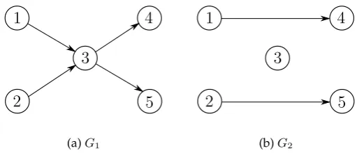
This section provides an example on a small-scale instance to show the effect of taking congestion into account in multicommodity network design. Assume a five node instance, as given in Figure 1, where all links have unit capacities and unit fixed-charge costs. The two links into and the two out of node 3 have unit flow costs, links 1–4 and 2–5 have unit flow cost of 10 each. There are two commoditiesp1andp2to be shipped, withwp1 = 1,o(p1) = 1,d(p1) = 4andwp2 = 1,o(p2) = 2,

d(p2) = 5. We assume that node 3 in the network is a transhipment point (e.g., a rail-yard) with a delay cost arbitrarily set equal toD3 = 5given that the total congestion cost increases linearly with this parameter. The capacity of node 3 has initially been set equal to the total amount of commodity flows in the network, which is c0

destination points with Di = 0, i = 1,2,4,5 as they are either origin or destination nodes, for

which neither capacity nor congestion is relevant for the purposes of this numerical example. We also assume the following initial settings on parametersα = 3,β = 3andF = 1, but the effect of changing the former two parameters against the capacity of node 3 will be shown later.

Figure 1: A five node MCND instance

An MCND solution on the sample 5-node instance is given in Figure 2(a) where both commodities go through node 3 with a total cost of 8 units consisting only of flow and fixed-charge costs. However, if one calculates the “hidden” cost of congestion through function (3), the overall cost rises to8 + 5(2 + 3(24/23)) = 48units. Alternatively, a solution minimizing the total cost including congestion is given in Figure 2(b) wherein the commodities are shipped from their origins to their destinations as direct deliveries. The total cost of this solution is 22 units.

(a)G1 (b)G2

Figure 2: Two solutions on the sample instance: (a) minimizing fixed and flow costs and (b) minimizing congestion at node 3

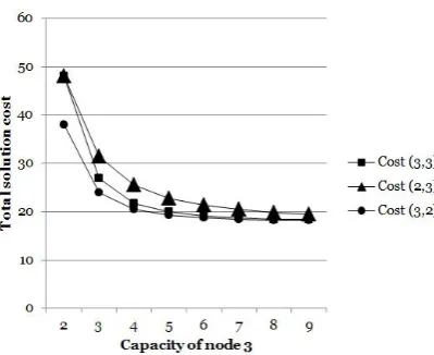
The two solutions shown in Figure 2 are two extreme cases one might encounter. The solutions obtained will certainly vary with the parameters chosen for the congestion function but the ex-ample shown here serves to illustrate cases where incorporating a congestion function into this problem might significantly change the structure of the solution on the same instance. To provide more information as to how the total cost of the solution changes with varying values of some of its input parameters, we present Figure 3.

Figure 3 shows the shape of the total solution cost comprising fixed, variable and delay costs in the vertical axis against varying values of initial capacityc0₃ in the horizontal axis. The total cost is shown by Cost (α,β) as a function of the two calibration parameters. It is clear from the figure that the total cost starts to level off whenc0₃exceeds a certain value, which, in this case is between 5 and 6. In fact, both solutions shown in Figures 2a and 2b become alternative optima for Cost (3,3) whenc0

Figure 3: Congestion function with different values ofαandβ

c0₃ = 2is increased by a single unit.

The following section presents the development of a mathematical model for the cMCNDP.

4. Mathematical Formulations

In this section, a notation of the problem is summarised followed by the mathematical formula-tion. The following decision variables are defined to model the cMCND. Letxp_ij ≥ 0denote the amount of flow of commodityp∈ Pon arc(i, j)∈ A. The binary variables of the model are given below:

yij =

{

1 arc(i, j)∈ Ais used.

0 otherwise, (4)

zi=

{

1 if nodei∈ N is upgraded

0 otherwise. (5)

The following sets are used in the model:

• A: set of arcs,

• P: set of commodities, • N: set of nodes.

The list of parameters used in the model are as follows:

• ei: fixed cost of upgrading the nodei∈ N,

• fij: fixed cost of establishing (opening) an arc(i, j)∈ A,

• dp_ij: the unit cost of routing the demand for commodityp∈ Pover arc(i, j)∈ A,

• c0_i: the initial capacity of nodei∈ N,

• wp: the quantity of commodityp∈ Pto be shipped,

• uij: the capacity of an arc(i, j)∈ A,

• Di: the delay cost of nodei∈ N,

• Fi: the free flow classification delay for nodei∈ N,

• α, β: calibration parameters,

• vi: the total amount of flow into nodei∈ N.

Given the notation above, a mathematical programming formulation for the problem is presented below:

M Minimize ∑

(i,j)∈A

fijyij +

∑

(i,j)∈A

∑

p∈P

dp_ijxp_ij+∑

i∈N

eizi+

∑

i∈N

gi(x, z) (6)

subject to ∑

j∈N_i+

xp_ij− ∑

j∈N_i−

xp_ji=dp_i ∀i∈ N, p∈ P (7)

xp_ij ≤wpyij ∀(i, j)∈ A, p∈ P (8)

∑

p∈P

xp_ij ≤uijyij ∀(i, j)∈ A, (9)

∑

j∈N−

∑

p∈P

xp_ji≤c0_i +cδ_izi ∀i∈ N, (10)

yij ∈ {0,1} ∀(i, j)∈ A (11)

xp_ij ≥0 ∀(i, j)∈ A, p∈ P (12)

zi∈ {0,1} ∀i∈ N. (13)

In formulationM, the objective function represents the total cost of design, routing and capacity augmentation and cost of congestion. The functiongi(x, z) that appears in the last term of the

objective function models congestion and is expressed as follows,

gi(x, z) =Di

         Fi ∑

j∈N−

∑

p∈P

xp_ji+β

  ∑

j∈N−

∑

p∈P

xp_ji

 

α+1

(c0

i +cδizi)α

         , (14)

whereαandβare calibration parameters.

its initial (i.e.,zi = 0) or extended (i.e.,zi = 1) capacity. Integrality and nonnegativity restrictions

on the decision variables are given by (11)–(13). ModelMhas the structure of a nonlinear, mixed integer, multicommodity network design problem including congestion effects and upgrading decisions at nodes.

The following section will present a conic mixed integer programming formulation. The latter re-quires the following notation change in the problem formulation. We first introduce an additional variable,vi ≥ 0, which denotes the total amount of flow into node i ∈ N. The new variable is

expressed, in mathematical terms, as follows:

vi =

∑

j∈N−

∑

p∈P

xp_ji ∀i∈ N. (15)

Under the new variable definition, the congestion function becomes

gi(v, z) =Di

(

Fivi+β

(vi)α+1

(c0

i +cδizi)α

)

.

In the following sections, we describe two methods for the problem, namely a conic mixed integer programming reformulation ofM, and an evolutionary algorithm, in the given order.

4.1. MISOCP reformulation

FormulationMgiven in Section 4 is a mixed integer nonlinear programming problem due to the second termg(v, z)appearing in the objective function. For the purposes of the reformulation, we represent the nonlinear part ofg(v, z) bygnl_{(v, z)as shown below (indicesiare dropped for the}

sake of simplifying the exposition).

gnl(v, z) =Dβ (v)

α+1 (c0_+cδ_z)α.

The function gnl_{(v, z) gives rise to two congestion cost functions, g}nl_{(v,0)and g}nl_(v,1),

corre-sponding to capacity levelsc0(i.e.,z= 0) andc0+cδ(i.e.,z= 1), respectively. Figure 4 illustrates these two cost functions.

Figure 4: Congestion Costs at Different Capacity Levels

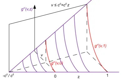
given that α > 1. Whenz is not fixedgnl(v, z) defines a surface. Figure 5 presents the surface defined bygnl(v, z)when restricted by the constraintv≤c0+δz.

Figure 5: Surface Defined bygnl_{(v, z)}

andv≤c0_+cδ_z

In this section, we show that we can reformulateMas a conic mixed integer programming for-mulation, for which the following result will be used.

Proposition 1. gnl(v, z)is a Second Order Cone Programming (SOCP)-representable function.

Proof. A function is SOCP-representable if its epigraph is so. Hence, we consider the following inequality

Diβ

(vi)α+1

(c0

i +cδizi)α

≤t ∀i∈ N. (16)

Inequality (16) can be equivalently written as

Diβviα+1 ≤t·(c0i +cδizi)α ∀i∈ N, (17)

which is of the form

r2l≤s1s2· · ·s2l, (18)

forr, s1, . . . , s2l ≥ 0. Inequalities of form (18) are SOCP-representable (Ben-Tal and Nemirovski,

2001). We can express inequality (18) by usingO(2l)variables andO(2l)hyperbolic inequalities of the form

u2 ≤v1v2, u, v1, v2 ≥0. (19)

Each hyperbolic inequality (19) can be written as a second-order conic inequality

∥(2u, v1−v2)∥ ≤v1+v2. (20)

Thus,gnl(v, z)can be represented via SOCP constraints.

G ¨urel (2011) has shown that a widely used form of congestion functions, which is a class of convex power functions, can be represented via second-order conic inequalities. The same author has also shown that, due to the polyhedral characteristics these functions have, they can be efficiently computed in network flow problems. We observe thatgnl_{(v, z) fall into this class and hence we}

As given in the proof of Proposition 1, when reformulating the problem, we first replacegnl(v, z) with an auxiliary variable t ≥ 0, following which we include the SOCP representation of in-equality (16) in our formulation. Example 1 shows how the SOCP representation for an example functiongnl(v, z)can be obtained.

Example 1. Consider a congestion cost function in whichα= 3₂,Diβ = 1,c0i = 2andcδi = 3. Then,

inequality (16) becomesv5/2 ≤t(2 + 3z)3/2, which can be equivalently written asv5/2 ≤ty3/2and

y= 2 + 3z. The former is equivalent tov5_≤t2_y3_{, which can be rewritten as,}

v8 ≤t2y3v3, (21)

which is a special case of inequality (18).

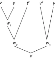
In order to obtain the SOCP representation of inequality (21), we follow the construction of Al-izadeh and Goldfarb (2003). In particular, we build the inequality (21) by using a binary tree with leaf nodes for{t, t2, t4, . . .},{y, y2, y4, . . .}, and{v, v2, v4, . . .}. Then, using the binary representa-tion of the exponents oft2, v3, andy3on the right hand side of inequality (21) we form the leaves of the construction tree as shown in Figure 6. Note that, in order to express an integer exponent, we only use powers of 2 as the leaves of the binary tree. Each non-leaf node of the binary tree represents a new hyperbolic inequality (19) and the new variable introduced.

Figure 6: Binary Representation Tree for Example 1

Using the construction above, we can express inequality (21) equivalently through the following set of hyperbolic constraints:w2₁ ≤vy,w2₂ ≤w1t,w1≥0,w32≤vy,v2 ≤w2w3,w2 ≥0andw3 ≥0. One can easily check this equivalence by squaring the last inequality twice to achieve v8 on its left-hand side and then substituting wi’s on the right-hand side appropriately. The hyperbolic

constraints are then written in SOCP form as: ∥(2w1, v−y)∥ ≤ v +y,∥(2w2, w1−t)∥ ≤ w1 +

y,∥(2w3, v−y)∥ ≤v+y,∥(2v, w2−w3)∥ ≤w2+w3.

As a result,Mcan be reformulated as follows,

MM ISOCP Minimize

∑

(i,j)∈A

fijyij +

∑

(i,j)∈A

∑

p∈P

dp_ijxp_ij+∑

i∈N

eizi+

∑

i∈N

DiFivi+Diβti, (22)

subject to (7)–(9), (11)–(15), and

5. Solution Procedure

This section describes an evolutionary algorithm for the cMCNDP. Recently proposed heuristic methodologies for the traditional MCNDP use a trajectory-based algorithm (Ghamlouche et al. 2003, Crainic et al. 2006) or an evolutionary framework (Ghamloucheet al. 2004, Alvarez et al. 2005) to select the arcs of the network, following which an off-the-shelf optimizer is used to solve the linear programming flow problem on the network configuration. In this paper, a similar ap-proach is followed, although in this case the flow problem that arises within the algorithm is non-linear. The details of the algorithm and the way in which the nonlinear subproblem is handled is explained below.

The solution methodology is an adaptation of the Cycle-based Evolutionary Algorithm (CEA) proposed by Paraskevopoulos et al. (2014), in which additional decisions and aspects that the cMCNDP introduces are taken into account. In particular, a tailor-made cMCNDP evolutionary algorithm is proposed wherein (a) the solution recombination takes into account both node up-grading decisions and links establishments from the parent solutions to produce offspring (b) an efficient perturbation strategy is used that uses long term memory to guide the search towards unexplored regions of the solution space, (c) and the local search employs new neighbourhood operators that explicitly consider congestion at nodes.

Algorithm 1:Evolutionary Algorithm

Input:λ(initial population size),µ(Reference Set size),ψ(number of local search iterations without an improvement),κ(Candidate Set size),ϑmax(number of SOCP solver calls

within local search without an improvement)

Output: Reference Set(R), sbest∈R

1. Initialization phase

R←ConstructionHeur(λ, µ);

whiletermination conditionsdo

2. Scatter Search phase

M ← ∅, M ←SolutionCombination(κ, µ); 3. Education phase

forindividualsofM do

s′←ILS(s, ψ, ϑmax);

UpdateRefSet(R, s′);

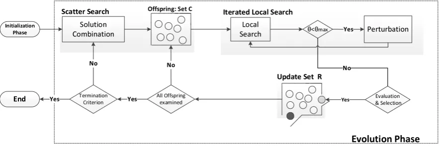
In summary, the evolutionary algorithm is based on principles of Scatter Search (SS) and inte-grates an Iterated Local Search (ILS) as an improvement, or an “education” method. Within the algorithm, the basic three-phase SS scheme is followed, namely (i) initialization, (ii) scatter search to produce offspring, (iii) education phase using the ILS. These steps will be described in greater detail below. A pseudecode of the overall framework is presented in Algorithm 1.

Figure 7: The flow chart of the Evolutionary Algorithm

5.1. Initialization phase

Theinitialization phaseuses a constructive heuristic to initialize a pool ofµdiversified and good-quality solutions, which are hosted in the Reference SetR. A serial construction procedure routes a particular commodity at each iteration, and finds the best path for that commodity by considering options of splitting or routing the total amount as a whole. The paths are found by using Dijkstra’s shortest-path algorithm. A greedy function is used that considers the fixed and flow cost of the arcs, as well as the congestion and upgrading costs on the nodes, and ensures that arcs and nodes capacities are always satisfied. Given the set of open arcs and the upgraded nodes, i.e., the 0– 1 decision variables yij and zi fixed in formulation MM ISOCP, the resulting flow problem is a

SOCP formulation which is solved by a SOCP solver. Its solution provides an optimal flow of commodities on the network.

This algorithm also handles the decisions on whether to upgrade a node or not internally as fol-lows. At any iteration of the Dijkstra algorithm, let the end node of a given arc be a candidate that is to be assigned a permanent label. Then, two congestion costs are calculated for this node; one that assumes a capacity upgrade on the node, and one that does not. Then, the procedure will assign a permanent label to the node that has the least total cost, including both the arcs costs and the congestion costs at nodes. If at a particular iteration a node is chosen to be upgraded, it will remain upgraded until the construction heuristic terminates and a complete solution is derived.

5.2. Reference Set Updating Criteria

There are certain criteria according to which the Reference SetRis updated with new solutions. The goal is to maintain a balance between quality and diversity and to avert premature conver-gence. A new solution is inserted intoRif it is better than the ever best found in terms of the total cost, or if it increases the average dissimilarity of theR and its cost is better than the worst-cost solution inR. In both cases, the worst cost solution inRis removed and the new solution is in-serted. To calculate the dissimilarity of theR, the current solution is temporarily inserted intoR

and the worst-cost solution inRis temporarily removed. The distance of all pairs of solutions is estimated by the Hamming distance, which is computed by considering both the arcs of solutions and the upgraded nodes, and is given by the formula below:

H(s, s′) = ∑

(i,j)∈A

|ys_ij−ys_ij′|+∑

i∈N

where, for a given solutions,y_ijs is a binary variable equal to1if arc(i, j)∈ Ais open, or0if not. Similarly,z_isis a binary variable equal to1if nodei∈ N is upgraded, or0if not.

5.3. Scatter Search Phase

In the scatter search phase, R is evolved via an efficient solution combination method and an improvement method, namely the ILS. A subset generation method randomly selectsκsolutions fromRrepeatedly, andµoffspring are produced based on scatter search principles. ILS attempts to improve the quality of each offspring, before the latter can be inserted intoR according to the elitist update criteria described in Section 5.2.

5.3.1. Solution Combination method

The proposed solution combination method combines the solution elements of κ solutions se-lected fromR to form the Candidate Set (C). These elements are both the arcs and nodes of the solutions. Each arc and each node status, i.e., open (or closed) and upgraded (or not upgraded) respectively, are assigned a value of preference. To calculate this value of preferenceκweights are introduced, as many as the number of solutions inC. If an arc (or node) is found open/closed (or upgraded/not upgraded) in more than one solution, the value of preference of its status is calcu-lated as the sum of the respective weights. A voting procedure is incorporated to determine which status is the dominant for each arc and for each node, according to the formulae given below:

Arc preferences: Opij=

∑

s∈C

y_ijs

f(s) +γhits(s) Clij =

∑

s∈C

1−y_ijs

f(s) +γhits(s) ∀(i, j)∈ A,

(25)

Node preferences: U pi =

∑

s∈C

zs_i

f(s) +γhits(s) nU pi =

∑

s∈C

1−z_is

f(s) +γhits(s) ∀i∈ N, (26)

whereγis a positive normalization parameter, i.e., average cost of an arc in the best so far solution found,OpijandClijare the scores for the open and closed status, respectively, for the arc(i, j), and

U pi andnU pi are the scores for the status of the node i(upgraded or not). The first component

f(s) in the denominators of (25) and (26) is the cost of the solution s. The second component denotes the number of times a particular solutionshas participated in the recombination process. The latter is used for diversification purposes to prevent the recombination process from choosing frequently selected parents. The status with the higher value dominates, both for the arcs and the nodes.

The output of the above procedure is a preferable status for each and every arc and node. To build a feasible solution, one should determine also the commodities flows for each link, which is done through solving the associated non-linear programming flow problem as described above.

the flow cost tocij/L, whereLis a large constant. The preferred status for the nodes is assigned

in a subsequent step, where given the flows the upgrading decision might be made to preserve the capacity constraints at nodes. The latter overcomes the preferred status in case it is non-upgrade, at the expense of preserving the capacity constraints at nodes. Towards the other end, the reconstruction mechanism also incorporates a final check to see if there are any cost savings by down-grading any of the upgraded nodes, provided commodity flows still remain feasible.

5.3.2. Education phase

The offspring produced by the evolution phase are improved using ILS, applied to each individual offspring. ILS has two main components; a local search and a perturbation strategy. The proposed local search introduces new neighbourhood structures and uses short term memory to enable the escape from local optima. The perturbation strategy partially modifies the current solution according to information gathered during the search. The components of the ILS algorithm are shown in Algorithm 2.

Algorithm 2:Iterated Local Search

Input:s(current offspring),ψ(number of local search iterations without an improvement),

ϑmax(number of SOCP solver calls without an improvement) Output:s

ϑ←0,⃗h←0;

whileϑ < ϑmaxdo

⃗r←0 ;

s′ ←s

count= 1

whilecount < ψdo

N(s)←Neighbourhood Evaluation(s, ⃗r)

s←mins′′∈N(s)f(s′′)

Update Inefficient Chains(s′′) Update Memory Structures(s′′, ⃗r, ⃗h)

if{f(s)< f(s′)}then

count= 1

s′←s

else

count=count+ 1

s′ ←SOCPsolver(s′);

iff(s′)> f(s)then

s∗ ←Perturbation(s′,⃗h)

s←s∗;ϑ←ϑ+ 1;

else

ϑ←0;s←s′;

Algorithm 3:Neighbourhood Evaluation

Input:s(current solution),M a large number

Output:s′′(best neighbour) min =M;

forAll inefficient chainskofsand for all combinations of nodesi, jinkdo

PI ←ListCommodities(k, i, j); whilePIis not emptydo

ifisItFeasible(k, i, j,PI)then

s∗←GenerateNeighbour(k, i, j,PI); else

RemoveFirstCommodity(PI);Continue; if∆f_move(s, s∗)<minthen

s′′←s∗;min = ∆fmove(s, s∗); RemoveFirstCommodity(PI);

In evaluating the neighbours, the functionListCommoditiescreates a listPIof different

commodi-ties that flow between nodesiandjof an inefficient chaink, functionGenerateNeighbourgenerates a neighbour ofs′ by applying the flow rerouting, and functionRemoveFirstCommodityerases the first commodity of the listPI. Finally, the functionisItFeasiblereturns “true” if a particular

combi-nation (k, i, j) leads to a feasible re-routing of commodity flow. The complexity of Algorithm 3 is

O(|N |2), where|N |is the number of nodes.

The sections below describe the components of the ILS in greater detail.

5.3.3. Neighbourhood topology-structures

The local search within ILS utilizes compound moves, new neighbourhood structures, and fre-quency based memory to escape from local optima by penalizing previously visited neighbours. For this purpose, an array⃗rof size equal to the number of arcs is used to store the number of times an arc(i, j) ∈ Ahas participated in a local move. This number is used in the form of a penalty. Each time a better solution is found,⃗r is re-initialized to zero (Paraskevopouloset al., 2012). The following formulae depicts the local move cost:

∆fmove=f(s′)−f(s) +ρ

∑

(ij)∈A

bijrij, (27)

whereρis a normalization parameter, i.e., the average cost of an arc obtained by the best solution found, and bij a binary parameter equal to 1 if arc(i, j) has participated in a local move, and 0

otherwise.

chains. Inefficient chains are constructed using the following formula:

In(ij) =

∑

p∈Px p

ijcij+fij+gi(x, c, z) +gj(x, c, z)

∑

p∈Px p ij

, (28)

whereIn(ij)is an inefficiency measure of arc(i, j). The inefficient arcs are those whoseIn(i, j) values are higher than the average arc-inefficiency of the current solution. Inefficient chains are formed by connecting such arcs. Each pair of nodes (and not only the adjacent) along these chains are the nodes that participate into the local moves.

5.3.4. Node upgrading decisions

This section describes how node upgrading decisions are made within the ILS. Once an inefficient chain for flow rerouting is identified, all commodities that flow on the chain are selected. Alter-native paths, that these commodities can be rerouted on, are then identified by the Dijkstra-like algorithm mentioned above. Within this algorithm, the labeling process is carried out such that each path considers upgraded and regular capacities of the nodes on the paths, and permanent labels are given to those that minimize the total cost. Hence the upgrading decisions on nodes are made as the alternative paths are iteratively “built”. Once commodities have been rerouted from their original path to another, a further set of decisions are made for the upgraded nodes that appear on the original path as to whether downgrading results in better cost.

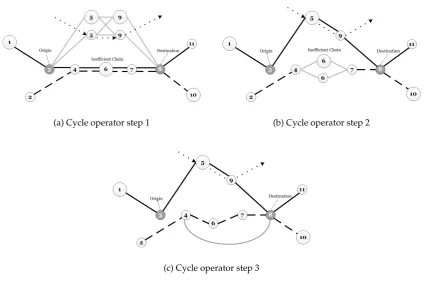
To be able to describe this process in greater detail, consider the example shown in Figure 8. In Figure 8a, two different commodities are considered, one flowing on the path shown by solid black lines (sayζ1) and the other flowing on the path shown by the dashed lines (sayζ2). Large nodes in the figure represent upgraded nodes, whereas the smaller ones are those which are not upgraded.

In this example, we assume that the path{3,4,6,7,8}define the part of the inefficient chain that will be subject to flow rerouting. Let an alternative path for reroutingζ1be identified as{3,5,9,8}. Both the arcs and the nodes on the alternative path are then duplicated. As seen in Figure 8a, although nodes 5 and 9 can accommodate the “dotted” commodity flow, it may still be worth upgrading one (or both) of the nodes to reduce the total cost. Figure 8b shows the next iteration, assuming that only node 5 is to be upgraded. At this point, node 6 on the original path is checked to see whether it should be downgraded to further reduce costs, as the flow running through this node has now been reduced due to the rerouting. Finally, Figure 8c shows that the flow of commodity

ζ2 is rerouted on an alternative path shown by the grey lines between nodes 4 and 8. At this point, the link costs of the original path are penalized to prevent the procedure from rerouting the commodity to its current path.

5.3.5. Perturbation

(a) Cycle operator step 1 (b) Cycle operator step 2

(c) Cycle operator step 3

Figure 8: A typical cycle-based local search operator

numbers, we perform a scaling down in all the elements of array⃗h, as soon as one of the elements of the array reaches a large numberQ. To guide the perturbation towards unexplored solutions in the search space, the cost of each arc (i, j)is multiplied by its score hij and the perturbation

is applied by considering the revised cost of each arc. The perturbation procedure is applied for

ψ/2 consecutive iterations, enough to be able to produce diversified solution structures but not long enough to “forget” the existing track record. The goal is to enable new arcs to participate to the current solution, which may have been neglected within the local search procedure, or even globally by the overall solution framework.

6. Computational Experiments

6.1. Generation of benchmark instances

The main goal was to define the initial capacity, upgrading capacity, upgrading cost and the unit congestion cost, in a way that the upgrading decisions will be driven by cost savings, as opposed to accommodating any excessive flow that the initial capacity of a node may not cope with. The parameters generated are node-specific, to reflect the practical situations where some nodes may be more expensive to upgrade, busier than others, or larger or smaller in terms of capacity. The heuristic algorithm was used to define the node parameters. The main idea behind this process was to identify the maximum and minimum flows that a node can accommodate by inspecting several good-quality and diverse solutions produced by the heuristic and comprising setB, and calculating the respective flow costs that each node has to cope with. The objective function cal-ibration parameters were set as follows: Di = 5andFi = 1for alli∈ N, andα = 3,β = 1. The

heuristic was run withψ= 30,θmax = 4andµ = 40. For this experiment, the algorithm was not

allowed to converge; instead it was run for three generations of the recombination process.

Initial capacities of the nodes are defined as 1.2 times maximum flow that flows into a node, as calculated from the elite pool of solutionsBproduced by the heuristic. The additional 20% is used as a safety margin to allow for higher values of flow, which might occur in solutions not discov-ered by the heuristic. As for incremental (upgraded) capacities, two settings were used: 30% of the initial capacity representing a minor upgrade investment, and 80% of the initial capacity cor-responding to a major investment. For the general experiments, parametersα, β,andFiremained

at3, 1and1 respectively. In an effort to normalize the order of magnitude of node and the arc costs,Di was defined as the maximum unit cost of flow that a nodeican accommodate. More

specifically, if for a given solutions, ys_ij is as defined before and (xp_ij)s is the amount of flow of commoditypon arc(i, j), then

Di = max s∈B

         ∑

j∈N_i−

fjiyjis +

∑

j∈N_i−

cp_ji(xp_ji)s

∑

j∈N_i−

(xp_ji)s

         . (29)

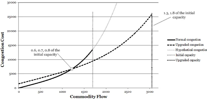
Finally, the upgrading cost is defined using the idea presented in Figure 9. In particular, this figure shows two graphs of the congestion function (14) for a particular node, one with and one without upgrading. The upgrading cost corresponds to an intersection point for these two functions, one that is between[0.5c0_i, c0_i]. We have chosen these values to be 0.6, 0.7 and 0.8 of the initial capacities, and calculated the upgrade cost as a result of solving a system of equations for calculating the intersection point for the three possible values.

Figure 9: Congestion graphs with and without upgrading

6.2. Computational experimentation with the MISOCP reformulation

This section reports of our computational experience with solving MM ISOCP, where all 258

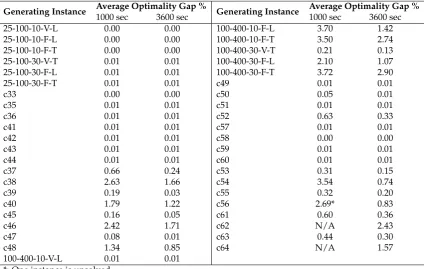
in-stances were attempted to be solved using CPLEX. To be able to see the effect of the computational running time on the solution quality, two limits of 1000 and 3600 seconds are imposed on the so-lution time. Table 1 presents average results, for each generating instance, the optimality gaps for each set of MCNDP instances, averaged across the six cMCNDP instances contained within each set. Full results are available and can be found athttp://www.apollo.management.soton. ac.uk/cMCNDPlib.htm.

As can be seen from Table 1, most instances can be solved to optimality using the MISOCP refor-mulation of the cMCNDP, shown by 0.00% or 0.01%, both of which are within the default optimal-ity tolerance settings of CPLEX. Instance set c56 had one instance for which CPLEX was unable to derive an integer feasible solution within the computational time limit of 1000 seconds. A similar situation was observed for all instances in sets c62 and c64. When the time limit was increased to an hour, all instances were either solved to optimality or a feasible integer solution with a gap of at most 2.9% was identified.

6.3. Computational experimentation using the evolutionary algorithm

6.3.1. Parameter calibration

The proposed evolutionary algorithm uses five parameters; the numberλof initial solutions ex-amined to produce the pool R of solutions, the size µ of the R, the size κ of the C, the maxi-mum numberψof local search iterations without an improvement in the solution quality, and the maximum numberϑmaxof CPLEX calls for which an improvement in the current solution is not

observed. The termination criterion for the algorithm is a computational time limit of one hour. The scaling parametersγandρare self-adjusted during the solution process, and are equal to the average cost of an arc in the current best solution found. The parameterλwas set equal to500, as it was found not to have significant impact in the algorithm’s performance. A further setting of

Table 1: Average optimality gaps for each group of cMCNDP instances

Generating Instance Average Optimality Gap % Generating Instance Average Optimality Gap %

1000 sec 3600 sec 1000 sec 3600 sec 25-100-10-V-L 0.00 0.00 100-400-10-F-L 3.70 1.42 25-100-10-F-L 0.00 0.00 100-400-10-F-T 3.50 2.74 25-100-10-F-T 0.00 0.00 100-400-30-V-T 0.21 0.13 25-100-30-V-T 0.01 0.01 100-400-30-F-L 2.10 1.07 25-100-30-F-L 0.01 0.01 100-400-30-F-T 3.72 2.90 25-100-30-F-T 0.01 0.01 c49 0.01 0.01

c33 0.00 0.00 c50 0.05 0.01

c35 0.01 0.01 c51 0.01 0.01

c36 0.01 0.01 c52 0.63 0.33

c41 0.01 0.01 c57 0.01 0.01

c42 0.01 0.01 c58 0.00 0.00

c43 0.01 0.01 c59 0.01 0.01

c44 0.01 0.01 c60 0.01 0.01

c37 0.66 0.24 c53 0.31 0.15

c38 2.63 1.66 c54 3.54 0.74

c39 0.19 0.03 c55 0.32 0.20

c40 1.79 1.22 c56 2.69* 0.83

c45 0.16 0.05 c61 0.60 0.36

c46 2.42 1.71 c62 N/A 2.43

c47 0.08 0.01 c63 0.44 0.30

c48 1.34 0.85 c64 N/A 1.57

100-400-10-V-L 0.01 0.01 *: One instance is unsolved

N/A: All six instances are unsolved

Q= 2000, which is the maximum value that an element of the arrayhtakes, before a scaling down of all the elements takes place.

Parametersψandϑmaxshould be defined so as to keep the total number of local search iterations

balanced with the number of generations produced within the available computational time limit. Our preliminary experimentation has showed that values of ϑmax equal to 6, 7, and 8 were

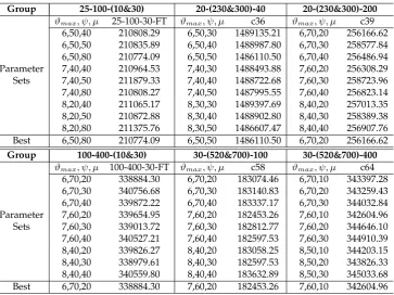
ap-propriate. Table 2 shows the results of the parameter calibration experimentation conducted on C and C+ sets of benchmarks instances to determine the best values ofϑmax,ψandµwith respect to

problem size. The instances are classified into six groups, according to the size of problems, and the label for each group, shown in the first line of Table 2, is a vector showing the number of nodes, the number of arcs and the number of commodities. For the experimentation, a single problem from each group was chosen, using the (0.3, 0.6) node configuration. As for the values tested, for large scale problems the reference set was assigned relatively small values and ψwas assigned high values, whereas the settings were the opposite for the small to medium scale instances.

pa-Table 2: Calibration of parametersϑmax,ψandµof the evolutionary algorithm

Group 25-100-(10&30) 20-(230&300)-40 20-(230&300)-200

ϑmax, ψ, µ 25-100-30-FT ϑmax, ψ, µ c36 ϑmax, ψ, µ c39

6,50,40 210808.29 6,50,30 1489135.21 6,70,20 256166.62 6,50,50 210835.89 6,50,40 1488987.80 6,70,30 258577.84 6,50,80 210774.09 6,50,50 1486110.50 6,70,40 256486.94 Parameter 7,40,40 210964.53 7,40,30 1488493.88 7,60,20 256308.29 Sets 7,40,50 211879.33 7,40,40 1488722.68 7,60,30 258723.96 7,40,80 210808.27 7,40,50 1487995.55 7,60,40 256823.14 8,20,40 211065.17 8,30,30 1489397.69 8,40,20 257013.35 8,20,50 210872.88 8,30,40 1488902.80 8,40,30 258389.38 8,20,80 211375.76 8,30,50 1486607.47 8,40,40 256907.76 Best 6,50,80 210774.09 6,50,50 1486110.50 6,70,20 256166.62

Group 100-400-(10&30) 30-(520&700)-100 30-(520&700)-400

ϑmax, ψ, µ 100-400-30-FT ϑmax, ψ, µ c58 ϑmax, ψ, µ c64

6,70,20 338884.30 6,70,20 183074.46 6,70,10 343397.28 6,70,30 340756.68 6,70,30 183140.83 6,70,20 343259.43 6,70,40 339872.22 6,70,40 183337.17 6,70,30 344032.84 Parameter 7,60,20 339654.95 7,60,20 182453.26 7,60,10 342604.96 Sets 7,60,30 339013.72 7,60,30 182812.77 7,60,20 344646.10 7,60,40 340527.21 7,60,40 182597.53 7,60,30 344910.39 8,40,20 339826.27 8,40,20 183058.25 8,50,10 344203.15 8,40,30 338979.61 8,40,30 182597.53 8,50,20 343826.33 8,40,40 340559.80 8,40,40 183632.89 8,50,30 345033.68 Best 6,70,20 338884.30 7,60,20 182453.26 7,60,10 342604.96

rameter setting for that particular group. This setting is applied to solve the rest of the problems in the group using a single run of the algorithm.

6.3.2. Computational results with the evolutionary algorithm

This section presents the results of the experiments where the evolutionary algorithm was com-pared with the results obtained using CPLEX. Full results are given in Table A.2 in the online appendix. A summary of the results is given in Table 3, showing averages for instances grouped into four on the basis of the number of nodes, being 20, 25, 30 and 100 shown under the first col-umn. In this table, the column shown by “Avg. Total Cost” shows the average total cost of all the instances with the corresponding number of nodes, obtained within the time limits of 1000 and 3600 seconds. In this table, we also report the average number of nodes upgraded under col-umn “UN”. The colcol-umn titled “Opt. Ratio” denotes the ratio of the number of instances solved to optimality out of the total number of instances tested within that group. The final column ti-tled “Deviations (%)”shows the percentage deviations of the solution values obtained with the heuristic from those obtained by CPLEX.

Table 3: Summary of the comparison results of the evolutionary algorithm with CPLEX

Nodes

CPLEX Evolutionary Algorithm

Deviations (%)

Avg. Total Cost

UN

Avg. Total Cost

UN

1000 sec. 3600 sec. Opt. Ratio 1000 sec. 3600 sec. Opt. Ratio 1000 sec. 3600 sec. 20 718089.6 718016.2 5.8 10/15 721457.6 720853.4 6.2 4/15 0.47 0.39 25 224316.2 224316.2 8.0 6/6 224509.7 224509.7 7.6 2/6 0.09 0.09 30 218804.2* 245114.0 8.9 7/16 250472.1 248272.1 10.6 0/16 - 1.27 100 269688.0 269301.2 13.8 2/6 272868.2 271802.2 14.6 0/6 1.17 0.92 *3 out of 16 solutions not found

6.4. Further numerical insight

6.4.1. Impact of congestion on the MCNDP solution

In this section, we provide further numerical insight on the impact that costs of congestion at nodes may have on the overall solution structure. The full results are presented in Table A.2 in the appendix, a summary of which are given in Table 4 where instances are grouped into four as in the previous section. These tables report statistics on the flow cost (AC), congestion cost (CC), total cost (TC) and the total number UN of upgraded nodes in the network. For a given instance, tests were conducted in the following way. First, the classical MCNDP is solved (columns 2–3 in Table 4). Then, using the solution of the MCNDP, a “manual” reconfiguration of the network to reduce the resulting congestion in the network by upgrading some nodes (columns 4–6) without changing the flows, which we call UpMCNDP. Finally, a cMCNDP is solved on the same instance (columns 7–10). The last two columns Dev1 and Dev2 show the percentage deviation of solution values of MCNDP and UpMCNDP from cMCNDP, respectively. The solutions for the MCNDP are taken from Paraskevopouloset al.(2014).

Table 4: Summary of comparison results between the classical MCNDP and the cMCNDP on benchmark instances of Gendron and Crainic (1994, 1996)

Group Avg. MCNDP Avg. UpMCNDP Avg. cMCNDP Deviations (%)

AC CC CC TC UN AC CC TC UN Dev1 Dev2 25 94613.0 151075.3 139760.9 234373.9 12.0 98045.6 126270.5 224316.2 8.0 −9.53 −4.48 20 291211.9 714609.3 604777.3 895989.2 14.7 339727.3 378285.6 718012.9 6.1 −40.08 −24.79 100 115502.7 189132.9 185185.3 300687.9 19.7 121178.0 148123.2 269301.2 13.0 −20.78 −11.65 30 94492.9 310417.8 240630.2 322717.5 24.3 119746.4 125367.6 245114.0 8.7 −65.19 −31.66

As Table 4 shows there are high congestion costs associated with the best solutions obtained for the classical MCNDP, which is obvious since congestion is not explicitly considered within this problem. The UpMCNDP approach is able to improve the situation by relieving congestion, im-plying improvements in the total cost from around 1% to 120%. The cMCNDP solution, on the other hand, is able to substantially improve on the MCNDP solutions, with the savings in cost ranging anywhere from 4.08% to beyond 200%. Interestingly, the flow cost (AC) in some cases, is seen to increase with cMCNDP but this is at the expense of obtaining a better TC. Finally, we observe that the number of upgraded nodes in cMCNDP is reduced in comparison to UpMCNDP, indicating that there is no need for upgrading so many nodes in the system. The results suggest that, instead of only upgrading nodes, a combination of upgrading with rerouting flows paths is a better way of alleviating congestion in the network.

tradi-Table 5: Statistics on capacity utilization of nodes for several problem instances

Instances

Average Capacity Utilization of Nodes

UpMCNDP cMCNDP

Avg. Max. Min. StDev. Avg. Max. Min. StDev. 20,230,40FT 0.530 0.715 0.229 0.206 0.484 0.641 0.245 0.157 20,300,40VL 0.591 0.845 0.260 0.181 0.504 0.641 0.183 0.159 30,520,100VT 0.591 0.965 0.404 0.101 0.473 0.653 0.274 0.130 100-400-10-VL 0.477 0.909 0.129 0.151 0.428 0.818 0.115 0.189 25-100-30-FT 0.567 0.813 0.459 0.083 0.539 0.632 0.265 0.148 25-100-10-FT 0.351 0.570 0.089 0.152 0.307 0.585 0.074 0.206

Table 6: Statistics on capacity utilization of arcs for several problem instances

Instances

Average Capacity Utilization of Arcs

UpMCNDP cMCNDP

Avg. Max. Min. StDev. Avg. Max. Min. StDev. 20,230,40FT 0.525 1.000 0.092 0.285 0.465 1.000 0.035 0.286 20,300,40VL 0.316 1.000 0.053 0.215 0.276 0.704 0.053 0.158 30,520,100VT 0.676 1.000 0.070 0.286 0.471 1.000 0.040 0.281 100-400-10-VL 0.544 1.000 0.056 0.311 0.519 1.000 0.014 0.344 25-100-30-FT 0.621 1.000 0.040 0.409 0.577 1.000 0.019 0.403 25-100-10-FT 0.624 1.000 0.074 0.396 0.628 1.000 0.049 0.410

tional MCNDP to the cMCNDP, we also present statistics on average (Avg.), minimum (Min.) and maximum (Max.) capacity utilization of nodes and arcs in Tables 5 and 6 for six different instances, as well as the standard deviations (StDev.). As this table shows, average capacity utilization on nodes decreases when the upgrading decisions at nodes are made and reaches lower levels in the cMCNDP solutions. Solving the cMCNDP typically results in an even distribution of the flows on the nodes and alleviates congestion, which consequently reduces arc capacity utilization as well.

6.4.2. Impact of different nodes’ settings on the upgrading decisions

The reasoning behind defining node properties (as discussed in Section 6.1) was to investigate on the impact different nodes capacities and upgrading costs would have on upgrading decisions, and generally on the cMCNDP solution itself. To test this reasoning further, we provide results of some experiments in Table 7 based on a selected set of instances. The first column of Table 7 shows the generating MCNDP instances with varying node properties in the second column. The third column of the Table gives the status of the solution. In particular, “Optimal” or “Opt.Tol.” indicates that an optimal solution was found. Otherwise the solutions are just “Feasible”. The last two columns are as defined previously.

Table 7: Computational results on problem instances with different node properties

Generating Instance Node properties Status TC UN

25-100-10-V-L

(0.3, 0.6) Optimal 30374.58 12 (0.3, 0.7) Optimal 30867.40 10 (0.3, 0.8) Opt.Tol. 31519.57 8 (0.8, 0.6) Opt.Tol. 29635.94 11 (0.8, 0.7) Opt.Tol. 30371.01 9 (0.8, 0.8) Optimal 31240.62 5

100-400-30-F-L

(0.3, 0.6) Feasible 130773.15 17 (0.3, 0.7) Feasible 131503.84 11 (0.3, 0.8) Feasible 132323.93 6 (0.8, 0.6) Feasible 129795.04 15 (0.8, 0.7) Feasible 131127.82 11 (0.8, 0.8) Feasible 132603.66 5

c44

(0.3, 0.6) Opt.Tol. 1545474.58 8 (0.3, 0.7) Opt.Tol. 1567386.50 5 (0.3, 0.8) Opt.Tol. 1586228.26 3 (0.8, 0.6) Opt.Tol. 1517143.54 7 (0.8, 0.7) Opt.Tol. 1548781.10 5 (0.8, 0.8) Opt.Tol. 1580478.01 4

c51

(0.3, 0.6) Opt.Tol. 129889.36 12 (0.3, 0.7) Opt.Tol. 131467.24 3 (0.3, 0.8) Opt.Tol. 131669.81 0 (0.8, 0.6) Opt.Tol. 128522.12 13 (0.8, 0.7) Opt.Tol. 130983.52 2 (0.8, 0.8) Opt.Tol. 131403.71 1

6.5. Real-life case study

To validate the proposed approach in a practical setting, we have applied it on a real-life (service) network design problem. The problem arises within the Polcorridor study (Polcorridor, 2006), which stems from a large European research project looking at the development of new rail-based intermodal transport solutions on the area of Northern Europe, and has already been considered in the relevant literature (Baueret al.2009, Andersenet al.2009, Andersen and Christiansen 2009). The problem consists of designing rail services to operate over three countries, namely Poland, Austria and the Czech Republic, with the main hubs being located in two ports in Poland and one in Vienna, between which goods are to be sent, for forwarding either to the northern or the southern European networks. The original network consists of 17 nodes, including 11 internal nodes in the three countries mentioned above, and the remaining external nodes that are beyond the boundaries of these countries and not included in the design problem. Figure 10 shows the map of the geographical region in which the problem is defined and the nodes that are part of the design. The reader is referred to Polcorridor (2006) and the above references for further details on the problem.

Figure 10: The Polcorridor supply system - Northern Europe

describe here. To apply the methodology, we first construct a time-space representation of the network, where each internal node{1, . . . ,11} is replicated fortperiods. In our case tis equal to 150, to cover from the time at which the earliest commodity becomes available until the latest possible time when all commodities can be sent to their destinations. There are 40 different types commodities to be transported on the network. Each commodity originates from a node on the network in the set{1, . . . ,11}and becomes available at a given point in time, which corresponds to a unique node in the time-space network corresponding to the spatial and temporal attributes of the commodity. Under the assumption that the commodities will need to be transported as quickly as possible, a dummy node was introduced into the the time-space network for each geographical

node{1, . . . ,11}, and connected to the replicas of these nodes in each time period (see Figure 11

for a visual depiction). To enable the model to favour “earlier” rather than “later” arrivals to destinations, the arcs(i, j)that connect the replicated nodes and the dummy node have variable costs equal toc_it_j∗

i = (0.1t

∑

i,j∈Acij)/|A|, whereitis thetthcopy of the internal nodei= 1, . . . ,11

in periodt andj_i∗ the dummy node of the same internal nodei. Each arc has its own variable cost, which is equal to the distance between the two nodes it connects. We do not consider any fixed costs for this case study as the arcs that correspond to the rail tracks are already in place. The time-space network representation contains a total of 1671 nodes and 8385 arcs.

For defining the capacity of the each arc, the Evolutionary Algorithm was run in the same way as was done for designing the benchmark instances (see Section 6.1). More specifically, the maximum flow that an arc could accommodate throughout these runs was multiplied it by 1.5 plus 40, i.e.,

vij = 1.5maxF low+ 40was used as capacity of the arc(i, j). Following the same procedure

Table 8: Computational results on the Polcorridor case study (Google Maps)

Scenario MCNDP UpMCNDP cMCNDP Deviations (%)

AC CC CC TC UN AC CC TC UN Dev1 Dev2 1671,8385,40 491546 9753891 7189239 7680785 181 495653 7101202 7596855 180 −1.10 −34.86

✁ ✂ ✁ ✄✁ ☎✁ ✆ ✁ ✝✁✁ ✝✂ ✁

✁ ✝ ✂ ✞ ✄ ✟ ☎ ✠ ✆ ✡ ✝✁ ✝✝ ✝✂

☛

☞

✌

✍

✎

✏

✑

✒

✓ ✔✕ ✖✗ ✘✙✚ ✘✛ ✔✜✢✕ ✣✔✤ ✥✖✚ ✦✙✧ ★✩✪ ✫✬✭ ✮✯✰✪ ✱✲ ✮✪ ✫✳ ✱✴ ✱✩✲✴✩✵ ✫✯✶✱✷ ✫

Figure 12: Upgrading decisions of nodes at different points in time

Table 8 reports the results of the Polcorridor case study. The table has an identical structure to that of Table 4. The reported results show that the congestion cost is significantly high in the MCNDP solution as compared to that of cMCNDP, i.e., the difference between the total cost of the solutions is−34.86%. Even when one uses the MCNDP solution and “manually” upgrades the congested nodes to reduce the resulting congestion in the network without changing the flows, the UpMCNDP solution deviates by−1.10% from to the solution obtained by solving the proposed cMCNDP.

The upgrading decisions (the number of which remained almost the same) are illustrated in detail in Figure 12. One can observe that most of the main (geographical) nodes need to be upgraded throughout a large part of the time horizon. Therefore rump up and rump down decisions can be made to minimize the total cost, following the upgrading decisions shown in Figure 12.

7. Conclusions

This paper presented and described solution methods for a variant of the multicommodity Net-work Design problem (MCNDP) where congestion at nodes is explicitly taken into account. The so-called congested MCNDP (cMCNDP) aims at finding flows for each type of commodity by ac-tivating suitable arcs and performing capacity upgrades at nodes, so as to minimize a function including operational and congestion costs, and by meeting capacity constraints on both arcs and nodes.