1
Nonlinear Minimum Variance Estimation
For Fault Detection Systems
Abstract
A novel model-based algorithm for fault detection (FD) in stochastic non-linear systems is proposed. The Nonlinear Minimum Variance
(
NMV) estimation technique is used to generate a residual signal which is then used to detect actuator and sensor faults in the system. The main advantage of the approach is the simplicity of the nonlinear estimator theory and the straightforward structure of the resulting solution. Simulation examples are presented to illustrate the design procedure and the type of results obtained. The results demonstrate that both actuator and sensor faults can be detected successfully.1. Introduction
The need for high performance, efficiency, safety and reliability in modern engineering systems has focussed interest in the Fault Detection and Isolation (FDI) problem. A fault is defined as an unexpected change in a system with component malfunction or variation in operating condition. Some faults, if not promptly and properly detected, could turn into unrecoverable failures, causing serious damage and even loss of human lives [1].
In the literature faults can be assume to take place in different parts of a system, and are classified as actuator faults or sensor faults [2]. Actuator faults can represent partial or complete loss of control action. A total actuator fault can occur as a result of a breakage, cut or burned wiring, short-circuit or the presence of foreign body in the actuator [2]. Sensor faults in incorrect outputs from the sensors. They can also be subdivided into partial and total faults.
Fault Detection (FD) methods can be classified into two major categories; model-based and data-driven approaches [3]. The model-based Fault Detection Isolation (FDI) approaches include parity space, parameter estimation and observer based approaches. The observer-based FDI method is one of the most effective and has received significant interest from industry [4]. Model based approaches typically rely on two steps: residual generation; the procedure of extracting fault symptoms from the process, and residual evaluation; the procedure of decision making [5]. The residuals are often generated using either an observer; for deterministic models, or an optimal filter for stochastic models.
2
Residual generation approaches have been developed successfully for linear systems. However, much less work has been done for nonlinear systems. This is primarily due to the complexity of nonlinear systems. The area of FDI for nonlinear systems is not covered completely yet, so it is worthy of study [7].
There is some existing literature on the use of a nonlinear estimator for fault detection and isolation. The most popular estimator for nonlinear processes is known to be extended Kalman filter (EKF) [8]. Although widely used, EKFs have some deficiencies, including the
requirement of differentiability of the state dynamics as well as susceptibility to bias and divergence in the state estimates. The unscented Kalman filter (UKF), on the contrary, uses the nonlinear model directly instead of linearizing it [9] and hence does not need to calculate the Jacobian and can achieve higher order accuracy. Particle filters (PF) or Sequential Monte Carlo Methods are considered a general numerical tool to approximate the a posteriori density in nonlinear and non-Gaussian filtering problems. The main drawback with the particle filter is that it is very demanding computationally[10].
In this study, the Nonlinear Minimum Variance (NMV) estimator is used for the first time to generate a residual signal for fault detection applications. The strong point of this technique is that a general nonlinear operator is used to represent the nonlinearity of the channel or of the measurement sensor. This might involve a set of nonlinear equations or even include a look-up table or be a model obtained from a neural or fuzzy-neural network. The main advantages of proposed estimator is that no on-line linearization is required, as in the extended Kalman filter, and implementation is easy. The cost-function to be minimized is the variance of the estimation error and a relatively simple optimization procedure and solution results [11].
The roadmap for this study is as follows. The derivation of NMV estimation method is given in section 2. NMV based residual generation for fault detection is described in section 3. The performance of the proposed fault detection method is illustrated by a case study in section 4. Finally the conclusions are summarised in section 5.
2. Nonlinear Minimum Variance Estimation
3
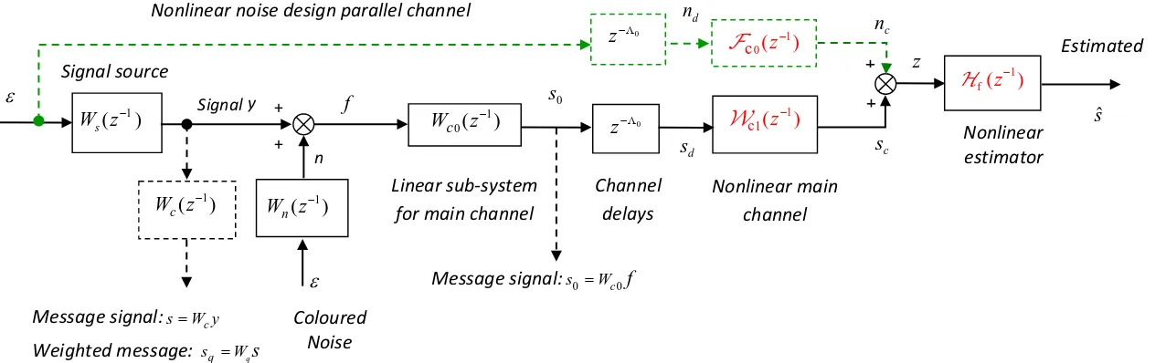
Figure 1: Signal and Noise Model and Communication Channel Dynamics
Estimated
1
( )
s
W z−
Signal source Coloured Noise n y Signal ε ε + + 1 ( ) n
W z−
1 1 c (z )
−
1
0( )
c
W z−
1 0
c (z− )
1 f(z )
− Nonlinear estimator z ˆ s
Nonlinear noise design parallel channel
Nonlinear main channel Linear sub-system
for main channel
+ + 0 z−Λ Channel delays c n c s f 0 z−Λ d s d n 0 s 1 ( ) c
W z−
Message signal:s=W yc Weighted message: sq=Wqs
[image:3.842.118.750.119.318.2]4
The signal channel model includes the nonlinearities that may involve both linear and nonlinear dynamics. The signal channel dynamics with a delay can be expressed as:
(
)
( )
(
0)
( )
0 1
c c
c hannelf t z W f t
−Λ
=
(1)
where z−Λ0 denotes a diagonal matrix of the k step delay elements in the signal paths and
0 = kI
Λ . The parallel path dynamics shown in Fig. 1, by a dotted line, can be expressed as:
0
0
1 1
c(z ) c (z )z
−Λ
− = −
(2)This is a fictitious channel, added to provide design tuning options, that can be used to represent uncertainties in channel knowledge, which provides additional design freedom. The
combined signal source and noise signal f ( t )∈Rr is given as:
f ( t )=y( t ) n( t )+ (3)
Consider the nonlinear system for the optimal estimation problem illustrated in Fig.1. The input and noise generating processes have an innovations signal model with white noise signal
input: ( )ε ∈t Rr and it may be assumed to be zero-mean with covariance matrix:
cov[ ( ),ε t ε τ( )]=Iδtτ where δtτ denotes the Kronecker delta-function. The signals shown in
the closed-loop system model of Fig.1 may be listed as:
Noise: n t
( )
=Wnε( )
t (4)Input signal: y t
( )
=Wsε( )
t (5)Channel input: f t
( )
= y t( ) ( )
+n t (6)Linear channel subsystem: s t0( )=
(
Wc0 f)
( )
t (7)Weighted channel interference: n tc( ) =(cε)( )t (8)
Nonlinear channel subsystem: s tc( )=
(
c1sd)
( )
t (9)Nonlinear channel input:
( )
0(
)
0( ) 0
d
s t = z−Λ s t =s t−k (10)
Observations signal: z t
( )
=n tc( )
+s tc( )
(11)Message signal to be estimated: s t( )=W y tc ( )=W Wc sε
( )
t (12)Weighted message signal: s tq( )=W W y tq c ( ) (13)
5
where ˆ(s t t−) denotes the estimate of the signal s(t) at time t, given observations z(t) up to
time t-. Value of may be positive or negative according to the following conditions: =0, for estimation; > 0, for prediction and < 0, for fixed-lag smoothing. The criterion for the nonlinear minimum variance estimator is given below:
{ { q ( | )( q ( | )) }}T
J =trace E W s t t − W s t t − (15)
where E{.} denotes the expectation operator and Wq[16] denotes a linear strictly
minimum-phase dynamic cost-function weighting function matrix which is assumed to be strictly minimum phase, square and invertible.
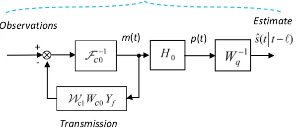
The estimate ˆ(s t t−) is assumed to be generated from a nonlinear estimator of the form:
1
ˆ( ) f( , ) ( )
s t t− = H t z− z t− (16)
where
1 1 1
0 0 c1 0
( , ) ( )
f t z W Hq c W Yc f
− = − + −
(17)
where f( ,t z−1) denotes a minimal realisation of the optimal nonlinear estimator. Since an
infinite-time (t= −∞) problem is of interest therefore no initial condition term is required.
The block diagram representation of f( ,t z−1) will be as shown in Fig. 2.
Figure 2: Implementation of the Nonlinear Estimator
The termsH , A and Y0 f used in equation (18) can be calculated using the concept of power
spectrum for the combined linear models using: φff =(Ws+W )(Wn s*+W )n* , and where the
notation for the adjoint of Ws implies: * 1 T
s s
W ( z− ) W ( z )= , and in this case the z denotes z-Transmission
Nonlinear estimator
- +
Observations Estimate
[image:5.595.146.445.487.619.2]6
domain complex number. The generalized spectral-factor: Yf may be computed using:
*
f f ff
Y Y =φ ,where Yf =A D0−1 f0 =D Af −1. The system models are assumed such that Df0 is
strictly Schur polinomial matrix [17, 18] satisfying:
0 0
* * *
f f s n s n
D D =( C +C )( C +C ) (18)
The right-comprime polynomial matrix model can be defined as:
1
f f q c s f
C D A− W W W Y
=
(19)
The polynomial operators H0 now may be optained from the minimal degree solution
0 0
( H ,F ), with repect to F0, of the following Diophantine equation:
0 0
k f
F A G z+ − −=C (20)
The estimation error can be penalised in a particular frequency range by using a dynamic
asymptotically stable weighting function WΩ =A BΩ−1 Ω, where A and BΩ Ωare polynomial
matrices. The weighted error involves a linear path at the optimum. In the linear case the modified cost function will have the form (Parceval’s theorem does not apply in the nonlinear case):
{
}
1
1 2
T *
ee z
J trace E(W e( t tΩ ))(W e( t tΩ )) trace / ( π j ) (WΩ W )dz / zΩ =
= − − = Φ
∫
(21)3. NMVE Based Fault Detection
In nonlinear minimum-variance estimation, the nonlinearities are assumed to be in the signal channel or possibly in a noise channel representing the uncertainty. The simple solution that follows arises because of the assumptions of linearity for the signal generating model and the results obtained here involve only a least-squares type of analysis [19].
7
Model-based FD methods are based on comparing the behavior of the actual signal and an estimated signal of the system. Typically, it is shown that in the absence of a fault, the observer residual approaches zero. When a fault exists, this residual will be non-zero, and it may therefore serve as a fault indicator.
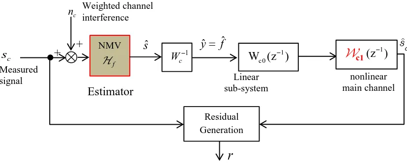
[image:7.595.110.524.207.373.2]The block diagram of the proposed nonlinear minimum variance estimator, taking =0, based on residual generation for fault detection, is shown in Fig. 3.
Fig. 3: NMVE Based Residual Generation Scheme
The residual signal can be generated by using measured signal
s t
c( )
and its estimateˆs t
c( )
, as:
r t
( )
=
s t
c( )
−
ˆ
s t
c( )
(22)The NMV algorithm estimates the signal
ˆs
soˆs
cmight be defined in term ofˆs
signal by usingeqn(6), eqn(7), eqn(9) and eqn(10) as follows
ˆ
y t
( )
=
W s t
c−1ˆ
( )
(23)ˆf t
( )
= ˆy t( )
=W s tc−1ˆ( )
(24)s tˆc
( )
=
c1W f tc0ˆ( )
(25)Then finally residual signal can be calculated substituting eqn(28) into eqn (23):
r t
( )
s tc( )
c1W W s tc0 c1ˆ( )
−= −
(26)This residual signal
r
is going to be checked with a reasonable threshold to detect that a fault has occurred in the system.NMV
f
Residual Generation
+ +
c
n
r
c s
Measured signal
ˆ
s
1 c0
W (z )−
c1(z )−1ˆc
s
Estimator
Linear sub-system
nonlinear main channel Weighted channel
interference
1
c
W−
ˆ ˆ
8
When there is a fault at the signal estimation point, the residual becomes
1 0
c1 ˆ
( ) c( ) c c ( ) f
r t =s t −
W W s t− +φ (27)c1W W s tc0 c1 ( ) c1W W s tc0 c1ˆ( ) φf
− −
=
−
+ (28)If the plant is linear this simplifies as:
r t( )=W W Wc1 c0 c−1
(
s t( )−s tˆ( ))
+φf (29)
=
W W W
c1 c0 c−1(
s( t t )
)
+
φ
f (30)Whereφfis a fault and where φf ≠0 is the output arising from the signal fault. However,
it can be only detected if term is large compared with estimation errors and the signal
noiseε
( )
t .3.1. Threshold computation
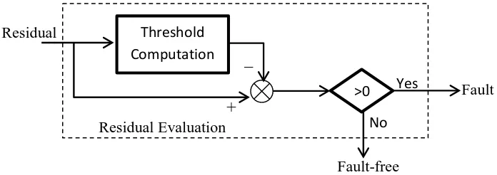
[image:8.595.111.459.468.591.2]To achieve a successful fault detection based on the available residual signal, further effort is needed. Residual evaluation and threshold setting are used to distinguish the faults from the disturbances and uncertainties. A decision on the possible occurrence of a fault will then be made by means of a simple comparison between the residual feature and the threshold, as shown in Fig. 4.
Fig. 4: Residual evaluation
In practice, the so-called limit monitoring and trend analysis are, due to their simplicity, widely used for the purpose of fault detection. For a given signal r, the primary form of limit monitoring is
min max
min max
if r T or r T then, Alarm, fault is detected
if T r T then, No Alarm, fault-free
< >
≤ ≤
Threshold Computation
Residual
+ _
>0 Yes No
Fault-free
Fault
9
where
T
min,T
max denote the minimum and maximum values of T in the fault-free case. Theyare the threshold values.
4. Design and Simulation Results
The computation of the estimator is relatively straightforward. The polynomial matrix equations can be solved using the Matlab polynomial toolbox PolyX. Given these matrices the estimator may be implemented very neatly, as shown in Fig. 2.
The selection of the uncertainty tuning function
c0 is a dual problem to the selection ofoptimal control cost function weightings [16]. The requirement for the nonlinear operator is that it should have a stable inverse. A simple starting point is therefore to assume the uncertainty model
c0 is a constant and of a small magnitude. This corresponds to thesituation where the uncertainty is simply white noise added at the output of the communications channel before it enters the estimator. Uncertainly is of course often associated with high frequency behavior and hence a simple linear lead term might be used to represent the frequency response of as in the example which follows.
To validate the effectiveness of the NMV filter based fault detection systems, nonlinear SISO system is used as an example. The NMV filter is computed below for the example and a simulation is used to verify the results.We consider a system having the following signal and noise models;
1
0 1 1 0 99 s
. W
. z−
=
− , 1
0 6 1 0 1 n
. W
. z−
= −
and let weighting Wq =1, Wc =0 5 1 0 5. − . z−1and Channel delay = z−1,so that Λ = =0 k 1.
The linear channel characteristics are defined as Wc0 =1 1 0 5( − . z−1). The static nonlinear
characteristic of the system is given in Fig. 5.
The dc-gain and changes in the cut-off frequency of the weighting filter
c0 influences theaccuracy of estimation.
c0−1 The tuning function , which is optimized for this example, hasthe following representation:
0
1 1
1
c
1 0.4 1 0.1
z z − −
−
− =
10
Fig. 5. Nonlinear Behavior of the Output Sub-System
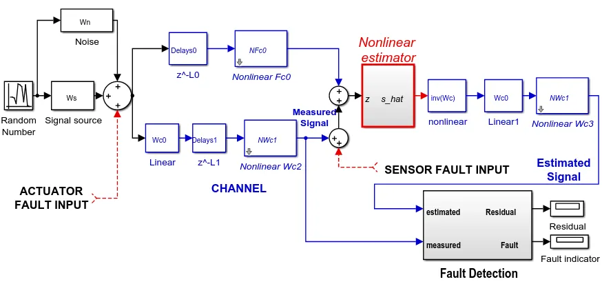
The overall system and simulink model of NMV filter for fault detection is as shown in Fig. 6.
Fig.6: Simulink Model of NMV Based Fault Detection Systems
Under normal operation condition (fault-free) measured signal and estimated signal are illustrated in Fig.7. The minimum variance for the NMV estimator is 1.14e-02. Tuning filter response is shown in Fig.8. Calculated residiual signal and confidence level threshold are dedicated in Fig.9. As shown in Fig. 9, residual signal is under the threshold. It means system is under normal operation.
-5 -4 -3 -2 -1 0 1 2 3 4 5
-5 -4 -3 -2 -1 0 1 2 3 4 5
input
out
put
system characteristics
Estimated Signal CHANNEL
SENSOR FAULT INPUT Measured
Signal
ACTUATOR FAULT INPUT
Ws
Signal source Random
Number
Wn
Noise
Residual
estimated
measured
Residual
Fault
Fault Detection Fault indicator
NWc1
Nonlinear Wc3
Wc0
Linear1
Delays0
z^-L0
NFc0
Nonlinear Fc0
Wc0
Linear
Delays1
z^-L1
z s_hat
Nonlinear estimator
NWc1
Nonlinear Wc2
inv(Wc)
[image:10.595.90.527.398.604.2]11
Fig.7. Measured and Estimated Signal (no fault)
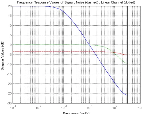
Fig.8. Tuning Filter Frequency Responses 0 50 100 150 200 250 300 350 400 450 500 -1
-0.8 -0.6 -0.4 -0.2 0 0.2 0.4 0.6 0.8 1
Time (Sec)
A
m
pl
it
ude
Measured Signal Estimated Signal
10-4 10-3 10-2 10-1 100 101 -30
-25 -20 -15 -10 -5 0 5 10 15 20
Frequency Response Values of Signal , Noise (dashed) , Linear Channel (dotted)
Frequency (rad/s)
S
ingul
ar
V
al
ues
(
dB
[image:11.595.181.425.338.534.2]12
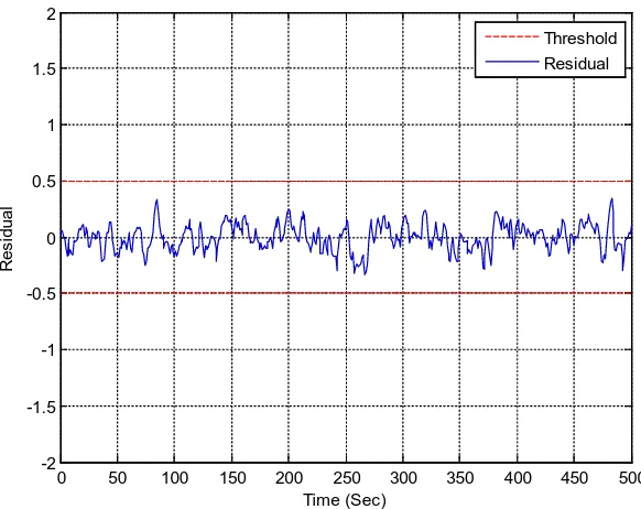
Fig.9. Residual Signal with Thresholds (no fault)
Two type of faults are applied to validate the effective of the proposed NMV estimator in fault detection implementation.
4.1. Sensor Fault
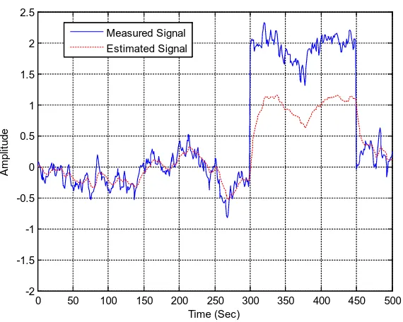
For the sensor fault; the signal shown in Fig. 10 is applied to the ‘sensor fault input’ of the system as illustrated in Fig. 6 simulink model. The fault is considered as a drift on the measurement sensor. After applied sensor fault, actual signal and estimated signal are illustrated in Fig. 11. Calculated residual signal and confidence level threshold are dedicated in Fig. 12. Fault has been detected successfully with accurate time as shown in Fig. 12.
0 50 100 150 200 250 300 350 400 450 500
-2 -1.5 -1 -0.5 0 0.5 1 1.5 2
Time (Sec)
R
es
idual
13
[image:13.595.158.443.376.604.2]Fig.10. Applied Fault Signal
Fig.11. Actual and Estimated Signal (faulty)
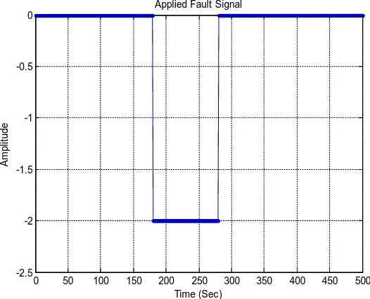
0 50 100 150 200 250 300 350 400 450 500 0
0.5 1 1.5 2 2.5
Time (Sec)
A
m
pl
it
ude
Applied Fault Signal
0 50 100 150 200 250 300 350 400 450 500
-2 -1.5 -1 -0.5 0 0.5 1 1.5 2 2.5
Time (Sec)
A
m
pl
it
ude
14
Fig.12. Residual Signal with Thresholds (faulty)
4.2. Actuator Fault
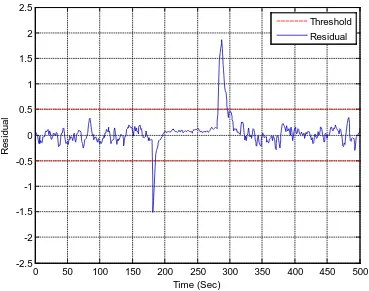
For the actuator fault; the signal shown in Fig. 13 is applied to the ‘actuator fault input’ of the system as illustrated in Fig. 6 simulink model. The fault is considered as a lost contact of the actuator input for a while. After the actuator fault is applied, actual signal and estimated signal are as illustrated in Fig. 14. Calculated residual signal and confidence level threshold are dedicated in Fig. 15. Fault has been detected successfully with accurate time as shown in Fig. 15.
Fig.13. Applied Fault Signal
0 50 100 150 200 250 300 350 400 450 500
-2.5 -2 -1.5 -1 -0.5 0 0.5 1 1.5 2 2.5
Time (Sec)
R
es
idual
Threshold Residual
0 50 100 150 200 250 300 350 400 450 500 -2.5
-2 -1.5 -1 -0.5 0
Time (Sec)
A
m
pl
it
ude
[image:14.595.161.424.486.699.2]15
Fig.14. Actual and Estimated Signal (faulty)
Fig.15. Residual Signal with Thresholds (faulty)
0 50 100 150 200 250 300 350 400 450 500 -3
-2.5 -2 -1.5 -1 -0.5 0 0.5 1
Time (Sec)
A
m
pl
it
ude
Measured Signal Estimated Signal
0 50 100 150 200 250 300 350 400 450 500 -2.5
-2 -1.5 -1 -0.5 0 0.5 1 1.5 2 2.5
Time (Sec)
R
es
idual
[image:15.595.114.483.440.731.2]16
5. CONCLUSIONS
A NMV estimator based fault detection system for nonlinear systems has been developed. The NMV estimator is used to generate the residual signal which indicates possible fault conditions in the system. The NMV estimator has some benefits relative to some other nonlinear estimators in three respects i.e. it requires less computational cost, easy to implement and to tune. The algorithm is illustrated using the simulation of a nonlinear process control example. The simulation results show that the method has a good performance in detecting faults at either inputs or outputs.
6. REFERENCES
[1] Alkaya A, Eker İ. Variance sensitive adaptive threshold-based PCA method for fault detection with experimental application. ISA Transaction ISA Transactions 50 (2011) 287– 302.
[2] Isermann R. Fault-diagnosis systems: an introduction from fault detection to fault tolerance. Berlin: Springer; 2006.
[3] Venkatasubramanian VR, Rengaswamy KY, Kavuri SN. A review of process fault detection and diagnosis, part I: quantitative model—based methods. Computers & Chemical Engineering 2003;27:293–311.
[4] Venkatasubramanian VR, Rengaswamy KY, Kavuri SN. A review of process fault detection and diagnosis, part II: qualitative models and search strategies. Computers & Chemical Engineering 2003;2:313–326.
[5] Chow, E. Y., and Willsky, A. S., 1984. Analytical redundancy and the design of robust failure detection systems. IEEE Transactions on Automatic Control, vol. 29(7):603–614.
[6] Hur, S.H., Katebi, R., Taylor, A., Model-based fault monitoring of a plastic film extrusion process. IET Control Theory Appl., 2011, Vol. 5, Iss. 18, pp. 2075–2088.
[7]Alrowaie, F., Gopaluni, R.B., Kwok, K. E., Fault detection and isolation in stochastic non-linear state-space models using particle filters. Control Engineering Practice, 20, (2012), 1016–1032
[8] Gerasimos G. R., A Derivative-Free Kalman Filtering Approach to State Estimation-Based Control of Nonlinear Systems. IEEE Transactıons On Industrial Electronics, Vol. 59, No. 10, 2012, 3987-3997.
[9] Mirzaee, A., Salahshoor, K., Fault diagnosis and accommodation of nonlinear systems based on multiple-model adaptive unscented Kalman filter and switched MPC and H-infinity loop-shaping controller. Journal of Process Control 22 (2012) 626–634.
17
[11] Grimble, M.J.,NMV optimal estimation for nonlinear discrete-time multi-channel systems, 46th IEEE Conf. on Decision and Control,New Orleans, 12–14 December 2007, pp. 4281–4286.
[12] Grimble, M.J.,Time-varying polynomial systems approach to multichannel optimal linear filtering’. Int. Conf. of Acoustics, Speech and Signal Processing, Detroit, MI, 9–12 May 1995, vol. 2, pp. 1500–1503.
[13] Grimble, M.J., Robust industrial control systems: optimal design approach for polynomial systems, John Wiley, Chichester, 2006.
[14] Grimble, M.J, 2011, 'Nonlinear Minimum Variance State Based Estimation for Discrete-Time Multi-Channel Systems', IET Journal on Signal Processing, Volume 5, Issue 4, July, Volume: 5 , Issue 4, Page(s): 365 – 378. Digital Object Identifier: 10.1049/iet-spr.2009.0064.
[15] Grimble M J, 2012, 'Nonlinear Minimum Variance Estimation for State-Dependent Discrete-Time Systems', IET Journal on Signal Processing, Volume 6, Issue 4, June, p. 379 – 391, DOI: 10.1049/iet-spr.2010.0220, Print ISSN 1751-9675, Online ISSN 1751-9683.
[16] Grimble M. J., Nonlinear generalised minimum variance feedback, feedforward and tracking control. Automatica, 2005, 41, 957-969.
[17] Kucera V., Discrete Linear Control, Wiley, Chichester,1979.
[18] Kucera V., Stochastic multivariable control:a polynomial equation approach, IEEE Trans.,1980,AC-25,(5),pp.913-919.