Nonlinear Minimum Variance Estimation for
Discrete-Time Multi-Channel Systems
Mike J. Grimble
, Fellow, IEEE
, and Shamsher Ali Naz
Abstract—A nonlinear operator approach to estimation in dis-crete-time systems is described. It involves inferential estimation of a signal which enters a communications channel involving both nonlinearities and transport delays. The measurements are assumed to be corrupted by a colored noise signal which is correlated with the signal to be estimated. The system model may also include a communications channel involving either static or dynamic nonlinearities. The signal channel is represented in a very general nonlinear operator form. The algorithm is relatively simple to derive and to implement.
Index Terms—Estimation, filtering, minimum-variance, non-linear, optimal estimation, optimization, quadratic cost.
I. INTRODUCTION
T
HE solution of linear filtering and estimation problems using least squares methods is well established and there are well accepted estimators like the Wiener [1] and Kalman filters [2], [3] that are often used. In this paper, the solution of a very special class ofnonlinear minimum variance (NMV) es-timation problems is considered. The main contribution lies in the definition of a simple estimator for systems with nonlinear communication channels containing delays. The generality of the problem is restricted to ensure a simple real time nonlinear estimator can be derived. The cost function to be minimized involves the variance of the estimation error and a relatively simple optimization procedure and solution results [4].The system of interest involves both linear and nonlinear sub-systems. The estimation problem considered here is to detect the signal of real interest given a measurement which includes noise. To allow for uncertainty, the measurement may also be as-sumed to include an interference signal that may enter through a parallel channel [5].
One of the main strengths of the technique is that the linear channel dynamics can be represented by a general non-linear operator. This might involve a set of nonnon-linear equations or could be a black box model containing unknown code and lookup tables. The model may even be obtained from a neural or fuzzy-neural network. The signal channel includes different
Manuscript received January 30, 2008; accepted January 28, 2009. First pub-lished March 10, 2009; current version pubpub-lished June 17, 2009. The associate editor coordinating the review of this manuscript and approving it for publi-cation was Prof. James Lam. This work was supported in part by the Engi-neering and Physical Sciences Research Council on the Platform Grant Project EP/C526422/1.
The authors are with the University of Strathclyde, Industrial Control Centre, Glasgow, G1 1QE, U.K. (e-mail: [email protected]).
Color versions of one or more of the figures in this paper are available online at http://ieeexplore.ieee.org.
Digital Object Identifier 10.1109/TSP.2009.2016999
delays and the resulting delayed output of the communications channel is assumed to be measured.
The measurement or observations signal also includes a noise signal which is assumed to derive from the same source but rep-resents uncertainty. This is modeled by a parallel communica-tions path which can represent a possible interference signal. This may not be a physical path but is included for design pur-poses to shape the interference and measurement noise atten-uation characteristics. The solution requires an assumption be made that a particular nonlinear operator has a stable inverse. This operator depends upon the nonlinear channel interference noise model, which is included for design purposes, and may therefore be freely chosen.
The structure for this paper is as follows. The nonlinear system and linear signal model, the cost-function and the solution of the optimal estimation problem are described in Section II and the main theorem is also introduced there. In Section III, a design example that includes nonlinearities is presented. Finally, conclusions are summarized in Section IV.
II. NONLINEARESTIMATIONPROBLEM
A nonlinear inferential estimation problem is considered involving the estimation of a signal, which enters a multi-channel communication multi-channel including nonlinearities and transport-delay elements [6], [7]. The measurements are as-sumed to be corrupted by a noise signal, which are correlated with the signal to be estimated for channels. Signal and noise models are assumed to have linear time-invariant model representations, which is not very restrictive, since in many applications the models for thesignalandnoisesignals are only
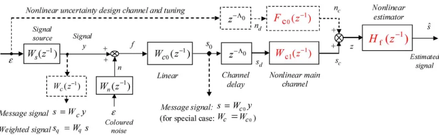
linear time-invariant approximations. The system, shown in Fig. 1, includes thenonlinearsignal channel model and linear measurement noise and signal models. These linear output models are in the same form as in the traditional linear optimal estimation problems [1], [2].
The message signal to be estimated is at the output of a linear block: . For greater generality a dynamic cost weighting is introduced and the weighted signal: is then to be estimated [8]. If the channel is identity and there is no uncertainty represented by the parallel dotted channel then this is similar to aWiener filteringtype of problem.
The polynomial matrix system models may be listed as
(1) (2)
where the unit delay operator is defined as . These models can be taken to be asymptotically stable. Note that the arguments of the polynomial matrices are often omitted
Fig. 1. Nonlinear filtering problem with noise sources, communications channel and channel interference.
for notational simplicity. The signal channel models can include severe nonlinearities that involve both linear and nonlinear dy-namics. However, the rest of the system description is defined so that simple results are obtained. The main nonlinear signal channel dynamics with different delays in different channels may be expressed as
(3)
where denotes a diagonal matrix:
of the common delay ele-ments in the respective output signal paths and .
A nonlinear parallel channel with dynamics and different channel time-delays may also be defined to have the form
(4)
This may be termed anuncertainty tuning function. The par-allel path dynamics in Fig. 1 are shown using a dotted line. This is because this channel will probably not exist physically but provides a signal that enters the cost-function to be introduced which enables the noise attenuation to be shaped. It is a ficti-tious channel which provides additional design freedom when the measurement noise characteristics are uncertain. If the gain goes to zero and the optimal estimator exists then this corre-sponds with the case where there is no channel uncertainty.
After separating the actual communications channel dy-namics into a linear input subsystem and a nonlinear model define the model for the main channel in the form
(5)
The output of the nonlinear subsystem with the explicit channel delays will be denoted as the signal: , where denotes time at the sample instants.
(6)
Note the following rather obvious signal notation is used: which will denote the signal delayed by dif-ferent amounts in difdif-ferent signal channels. For simplicity, the nonlinear subsystem: is assumed to befinite gain stable. For stability analysis, the time sequences can be considered to be contained in extensions of the discreteMarcinkiewicz space
[11]. This is the space of time-sequences with time-averaged square summable signals that have a finite power.
The input and noise generating processes have an innova-tions signal model with white noise signal input , and it may be assumed to be zero mean with covariance matrix , where denotes theKronecker delta-function. The combined signal source and noise signal
is given as
(7)
The infinite-time estimation problem where the filter is as-sumed to be in operation from an initial time: , is considered. The signals shown in the closed-loop system model of Fig. 1 may be listed as follows:
Noise (8)
Input signal (9)
Channel input (10)
Linear channel subsystem (11)
Channel interference (12)
Nonlinear channel subsystem
(13) Nonlinear channel input
(14)
Observations signal (15)
Message signal to estimate
(16)
Weighted message signal (17)
Estimation error signal (18)
In some problems, may represent part of the communica-tions path so that: . Thepower spectrumfor the com-bined linear models can be computed, noting these are linear
subsystems, using: , where the
notation for the adjoint of implies: ,
and in this case the denotes the -domain complex number. The generalized spectral-factor: may be computed using:
, where . The system
models are assumed to be such that is a strictly Schur, square, polynomial matrix [12] satisfying
Theright-coprimepolynomial matrix may now be defined as
(20)
Observe that the noise and signal models are correlated. How-ever, is normally low-pass and is normally high-pass and the results for the special case of the linear problem, with no channel dynamics, will be similar to those for the usualWiener
orKalman filteringcase [1], [2].
A. Proposed Solution for Nonlinear Estimation Problem
The estimation problem is concerned with finding the best es-timate of the signal in the presence of an interference noise term. The minimum variance optimal deconvolution problem
[13] involves the minimization of the estimation error
(21)
where denotes the optimal nonlinear estimate of the signal at time , given the observations: over the
semi-infinite interval: up to time . The
scalar may be positive or negative and as noted
Filtering
Fixed lag smoothing Prediction
The weighted estimation error cost-function which is to be min-imized has the form
(22)
where denotes the expectation operator and denotes a linear dynamic cost weighting function matrix which is as-sumed to be strictly minimum phase, square and invertible. The estimate is assumed to be generated from a nonlinear, estimator of the form
(23)
where denotes a minimal realization of the optimal non-linear estimator. Since an infinite-time problem is of interest no initial condition term is required. The following theorem applies.
Theorem: Optimal Estimator for Nonlinear Systems: The as-sumption is made that and commute and that the operator has a stable inverse. The nonlinear
deconvolution filter ,predictor , orsmoother
, to minimize the variance of the estimation error (22), for the system described in Section II, can be calculated from thespectral factor,Diophantine, and operatorequations. The
spectral factor , where is asymptotically
stable, is defined from the polynomial matrix
(24)
Right-coprime polynomial matrices and satisfy
[image:3.594.352.501.64.111.2](25)
Fig. 2. Nonlinear estimator structure.
The polynomial operators and may now be obtained from theminimal degreesolution , with respect to , of the following Diophantine equation:
(26)
Estimator: The optimal casual, nonlinear estimate
for the system described in Section II, to minimize the average variance of the estimation error (22), is given as
(27)
Minimum Cost: Theminimum variancemay be computed
(28)
Proof: The proof follows.
Remarks:
a) The assumption is required that ( and ) com-mute, which is certainly satisfied if the delays are the same
, or if these models are diagonal.
b) Note that theMinimum Variance follows from (28) for the system with uncertainty, and it does not, surprisingly, include the nonlinear sensor characteristics.
c) The structure for the resulting estimator is shown in Fig. 2.
B. Solution
To obtain an expression for the weighted estimation error
, note from the (7)–(9)
(29)
A realization of can be obtained using the spectral factor defined above as
(30)
where satisfies (19). Also recall the weighted message signal is given from (17) as
(31)
Estimation error: From equations: (1), (20), and (31), obtain
From (10), (12), (13), and (14) and obtain
(33)
Also using equations (11), (16), and (30)
Under the assumption that and commute, then
(34)
The first term may be simplified using the Diophantine equation and hence
(35)
C. Optimization
To compute theoptimal nonlinear estimator, first inspect the form of the weighted estimation errorin (35) and advance by
to obtain
(36)
The signal above will first be considered. The polynomial matrix term in (36) may be expanded as a sequence of terms
in the unit advance operator . It
fol-lows that the first term in (36) is dependent upon the future values of the white noise signal components
. The second group of terms in (36) (in the square brackets) are all dependent upon past values of the white noise signals, whereas the first term depends only upon future values. It follows that these two groups of terms are statistically independent and the expected value of the cross terms is null.
Also note that the first term on the right-hand side of (36) is in-dependent of the choice of estimator. It follows that the smallest variance is achieved when the remaining terms are set to zero.
Assuming the existence of a finite gain stable causal inverse to the nonlinear operator theoptimal estimatoris obtained by set-ting this second group of terms to zero, noset-ting
(37)
This completes the solution of the theorem.
Also note that assumption preceding the main theorem has to be satisfied for the results to apply so a silly choice of sensor characteristic would mean that the results would not hold. If the assumption does hold the minimum variance only depends upon the linear signal and noise model terms. The expression for the estimation error depends on both linear and nonlinear terms, however, all the nonlinear terms when combined with the nonlinear estimator add to zero. Thus, this cost may be consid-ered an ideal and if the uncertainty channel was null it would require an inverse to be computed for the sensor/channel char-acteristic. Thus, it appears independent of any sensor character-istic. In practice there will be uncertainty and the estimator will not try to cancel the nonlinear sensor/channel characteristic but the absolute minimum cost remains the same as defined by (28).
III. DESIGNISSUES ANDEXAMPLES
The computation of the estimator is relatively straightfor-ward. The polynomial matrix equations can be solved using the Matlab polynomial toolbox PolyX. Given these matrices the es-timator may be implemented neatly, as shown in Fig. 2. The NMV filter involves matrix calculations so its on-line computa-tional might be large but this is not true because the major matrix calculations are offline to be conducted during the design phase and these have no impact in the implementation phase. The com-putational complexity and implementation issues of the NMV filter are discussed in some detail in [25].
Fig. 3. Location of Lambda or oxygen sensor in automobile engine.
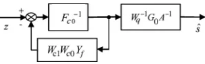
[image:5.594.43.536.247.734.2]Fig. 4. (a) UEGO Lambda sensor nonlinear behavior. (b) EGO Lambda sensor nonlinear behavior.
Fig. 5. Uncertainty tuning functionF frequency response for EGO sensor.
Fig. 6. Comparison between actual and estimated lambda using the EGO sensor.
In this particular example: Delay , where events and the signal and noise models
(38)
[image:5.594.306.548.257.451.2] [image:5.594.314.543.479.638.2]TABLE I USINGEGO SENSORONLY
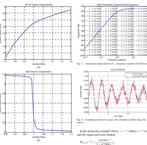
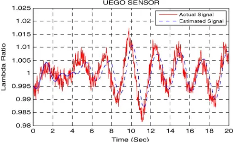
Fig. 7. Uncertainty tuning functionF frequency response for UEGO sensor.
Fig. 8. Comparison between actual and estimated Lambda using the UEGO sensor.
(40)
The universal exhaust gas oxygen (UEGO) sensor uses the changes of voltage that are representative of the oxygen levels in the reference and test chambers of the sensor to drive an elec-tronic control unit for feedback control. The exhaust gas oxygen (EGO) sensor is an alternative which is an electrochemical cell used to measure the oxygen content of an engine’s exhaust. In closed-loop operation this signal is used to monitor the fuel mix-ture. The static nonlinear characteristics of the UEGO and EGO sensors are shown in Fig. 4(a) and (b), respectively.
Three cases of the NMV estimation problem are now con-sidered. The minimum value of the cost for the system which includes uncertainty follows from (28) and may be computed as: . In first case the EGO sensor is used with the
[image:6.594.46.283.379.523.2]TABLE II USINGUEGO SENSORONLY
Fig. 9. Uncertainty tuning functionF frequency responses when EGO and UEGO sensors are used.
Fig. 10. Comparison between actual and estimated lambda.
uncertainty tuning function shown in Fig. 5, but the fictitious parallel uncertainty model is not included in the simulation, so the computed cost will not be expected to coincide with this the-oretical figure. The time response results are shown in Fig. 6 and Table I.
In the second case, the UEGO sensor was used and the results obtained in this case are shown in Figs. 7 and 8 and Table II. In the last case, both the EGO and UEGO sensors are used together and summed with two equally weighted estimators. The results obtained in this case are as shown in Figs. 9 and 10 and Table III. In all the above cases the estimator depends on the choice ofuncertainty tuning function to obtain a stable inverse of
TABLE III
USINGEGOANDUEGO SENSORSTOGETHERCOMPARISONWITH
[image:7.594.40.286.108.431.2]ALTERNATIVEAPPROACHES
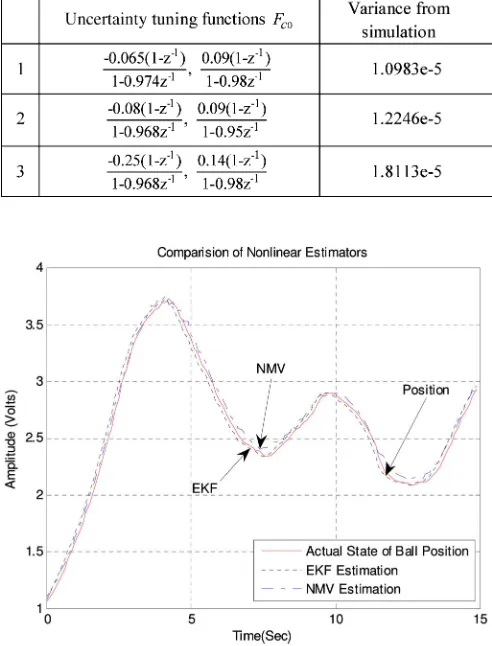
Fig. 11. Comparison results between NMV and EKF.
decreases so long as an optimal filter actually exists, which ex-plains much of the behavior in the table of values. The dynamic response should really reflect the type of uncertainty expected or if the parallel uncertainty channel exists then it will depend upon the physical model.
Comparison With Alternative Approaches: filtering: The minimax estimator for nonlinear systems may handle con-straints [22] and provides an alternative that may be particularly useful for systems with significant nonlinearities. The mixed and minimization problem enables traditional variance based estimation criteria to be considered but also allow uncer-tainty to be taken into account, considered by [23]. The most practical way to implement the estimator is in discrete form but there is a much greater level of mathematical abstraction in-volved [24].
Extended Kalman filter: A comparison is described in [21] and [25] that includes detailed discussions about the perfor-mance of NMV filter with the extended Kalman filter imple-mented on the ball and beam system in real time. The compar-ison results are shown in Fig. 11. The minimum variance for the NMV estimator was calculated as 0.00084 and for the EKF as 0.0035. We can also see from the Fig. 11 that the performance of the NMV estimator is good in comparison to the EKF and is in accordance with the minimum variance results.
The main strength of the approach is that for a restricted class of systems, where the technique is applicable, it provides a very simple solution to a difficult nonlinear estimation problem.
IV. CONCLUSION
The proposed nonlinear filter is applicable to a rather special class of nonlinear estimation problems. However, it is believed to be acceptable to reduce the generality of the problem consid-ered, to obtain a very practical nonlinear estimation algorithm. The solution is relatively easy to understand and to implement. For example, the theoretical basis, however restricted, is much easier to understand than or particle filtering, which is im-portant in applications.
Other nonlinear filtering techniques like the extended Kalman filter do of course involve approximations and they are not op-timal estimators. The solution proposed here does not involve the same type of approximation if the uncertainty tuning func-tion is representative. However, a quesfunc-tion of interest is whether the optimal estimator for the system containing the fictitious un-certainty model is more accurate than an approximately optimal estimator for the actual system. A comparison with an EKF in [21], using a Labview implementation, suggests the new class of estimators is good for a real application.
ACKNOWLEDGMENT
The authors would like to thank Dr. P .Majecki for his dis-cussions on applications and to the Engineering and Physical Sciences Research Council for financial support.
REFERENCES
[1] N. Wiener, Extrapolation, Interpolation and Smoothing of Stationary Time Series, With Engineering Applications. New York: Technology Press and Wiley, (first issued in February 1942 as a classified U.S. Nat. Defense Res. Council Rep.).
[2] R. E. Kalman, “A new approach to linear filtering and prediction prob-lems,”J. Basic Eng., pp. 35–45, 1960.
[3] R. E. Kalman, “New methods in Wiener filtering theory,” inProc. Symp. Engineering Applications of Random Function Theory Proba-bility, 1961, pp. 270–388.
[4] K. J. Åström, Introduction to Stochastic Control Theory. London, U.K.: Academic, 1979.
[5] M. J. Grimble and M. A. Johnson, Optimal Multivariable Control and Estimation Theory. London, U.K.: Wiley, 1988, vol. I and II. [6] M. J. Grimble, “Mutlichannel optimal linear deconvolution filters
and strip thickness estimation from gauge measurements,”ASME J. Dynam. Syst., Measurement Control, vol. 117, pp. 165–174, 1995. [7] M. J. Grimble, Robust Industrial Control: Optimal Design Approach
for Polynomial Systems. Chichester, U.K.: Wiley, 2006.
[8] M. J. Grimble, “Non-linear generalised minimum variance feedback, feedforward and tracking control,”Automatica, vol. 41, pp. 957–969, 2005.
[9] M. J. Grimble and V. Kucera, Polynomial Methods for Control Systems Design. London, U.K.: Springer-Verlag, 1996.
[10] M. J. Grimble, “Polynomial systems approach to optimal linear fil-tering and prediction,”Int. J. Control, vol. 41, no. 6, pp. 1545–1564, 1985.
[11] M. J. Grimble, K. A. Jukes, and D. P. Goodall, “Nonlinear filters and operators and the constant gain extended Kalman filter,”IMA J. Math. Control Inf., vol. 1, pp. 359–386, 1984.
[12] V. Kucera, Discrete Linear Control. Chichester, U.K.: Wiley, 1979. [13] T. J. Moir, “Optimal deconvolution smoother,”Proc. Inst. Electr. Eng.,
vol. 133, no. 1, pt. D, pp. 13–18, 1986.
[14] M. J. Grimble, Industrial Control Systems Design. Chichester, U.K.: Wiley, 2001.
[16] M. J. Grimble,inH Design of Optimal Linear Filters, MTNS Conf., C. I. Byrnes, C. F. Martin, and R. E. Saeks, Eds., Phoenix, AZ, 1987, pp. 553–540, 1988, North Holland, Amsterdam.
[17] M. J. Grimble and A. ElSayed, “Solution of theH optimal linear filtering problem for discrete-time systems,” IEEE Trans. Signal Process., vol. 38, no. 7, pp. 1092–1104, 1990.
[18] I. Yaesh and U. Shaked, “Transfer function approach to the problems of discrete-time systems:H optimal linear control and filtering,”IEEE Trans. Autom. Control, vol. AC. 36, no. 1, pp. 1264–1271, 1992. [19] M. J. Grimble, “H fixed-lag smoothing filter for scalar systems,”
IEEE Trans. Signal Process., vol. 39, no. 9, pp. 1955–1963, 1991. [20] U. Shaked, “H minimum error state estimation of linear stationary
processes,”IEEE Trans. Autom. Control, vol. 35, no. 5, pp. 554–558, 1990.
[21] S. A. Naz and M. J. Grimble,inUKACC Conf. Design Real Time Imple-mentation of Nonlinear Minimum Variance Filter, Manchester, U.K., Sep. 2008.
[22] D. Simon, “A game theory approach to constrained minimax state esti-mation,”IEEE Trans. Signal Process., vol. 54, no. 2, pp. 405–412, Feb. 2006.
[23] M. D. S. Aliyu, Boukas, and El-Kebir, “,” presented at the Discrete-Time Mixed H2/H-Infinity Nonlinear Filtering, American Control Conf., Seattle, WA, Jun. 11–13, 2008, Paper FrC17.1, unpublished. [24] S. Yuliar and M. R. James, On Discrete Time Nonlinear H-infinity
Filtering, Control. Barton, ACT, Australia: Institution of Engineers, 1995, vol. 95, pp. 295–299, National conference publication (Institu-tion of Engineers, Australia); no. 95/09.
[25] S. A. Naz and M. J. Grimble, “Design and implementation of nonlinear minimum variance filters,”Int. J. Adv. Mechatronic Systems, Jun. 2009, Paper Ref. No.: IJAMechS08036), to be published.
Mike J. Grimble(M’75–SM’78–F’93) was born in Grimsby, U.K. He received the B.Sc. (Coventry), M.Sc., Ph.D., and D.Sc. degrees from the University of Birmingham, U.K.
His research on the Industrial Automation Group at Imperial College was concerned with the mod-eling and control of cold strip mills. In 1981, The University of Strathclyde, Glasgow, U.K., appointed him to the Professorship of Industrial Systems, and he established the Industrial Control Centre more than two decades ago. His Centre is concerned with industrial control problems, particularly those arising in the automotive,
aerospace, process control, wind energy, metal processing, marine, electrical power and water industries. His research interests include nonlinear filtering and control systems, adaptive control, H robust, multivariable design, optimal control, and estimation theory.
Dr. Grimble is the Managing Editor of theInternational Journal of Adap-tive Control and Signal Processingand of theInternational Journal of Robust and Non-linear Control, and he was also recently appointed the Editor of Op-timal Control Applications and Methods, all published by Wiley. He was the Editor of the Prentice-Hall International series of books onSystems and Control Engineeringand also the Prentice-Hall series onAcoustics Speech and Signal Processing. He is currently a joint editor of the Springer Monograph Series on
Advances in Industrial Controland also the Joint Editor of the Springer text book series on Control and Signal Processing. He established a university con-sultancy company Industrial Systems and Control, Ltd., for which he acts as the technical director and also developed the Applied Control Technology Con-sortium, which is an international technology transfer and training organization with support from over 30 companies in Europe and North America. These have been successful in helping companies to adopt new technology for about two decades and they compliment the industrial research services of the centre. The Institution of Electrical Engineers presented him with the Heaviside Premium in 1978 for his papers on control engineering. In 1979, he was awarded jointly the Coopers Hill War Memorial Prize and Medal by the Institutions of Electrical, Mechanical and Civil Engineering. The Institute of Measurement and Control awarded him the 1991 Honeywell International Medal. He was awarded an IEEE Fellowship in 1992, and he was recognized at the 1993 Edinburgh International Science Festival as one of Scotland’s four most cited Scientists. He was ap-pointed a Fellow of the Royal Society of Edinburgh in 1999. He was awarded jointly the Asian Journal of Control best paper award for 2002–2003. He was re-cently awarded the Institution of Engineering and Technology Heaviside Medal for achievements in Control in 2008.
Shamsher Ali Nazwas born in Pakistan on January 1, 1970. He received the B.Sc. degree in electrical engineering from the University of Engineering and Technology, Lahore, in 1993. He is currently working towards the Ph.D. degree in the University of Strathy-clyde, Glasgow, U.K.