Proof-relevant parametricity
?Neil Ghani, Fredrik Nordvall Forsberg, and Federico Orsanigo University of Strathclyde, UK
{neil.ghani, fredrik.nordvall-forsberg, federico.orsanigo}@strath.ac.uk
Abstract. Parametricity is one of the foundational principles which underpin our understanding of modern programming languages. Roughly speaking, parametricity expresses the hidden invariants that programs satisfy by formalising the intuition that programs map related inputs to related outputs. Traditionally parametricity is formulated with proof-irrelevant relations but programming in Type Theory requires an exten-sion to proof-relevant relations. But then one might ask: can our proofs that polymorphic functions are parametric be parametric themselves? This paper shows how this can be done and, excitingly, our answer requires a trip into the world of higher dimensional parametricity.
1
Introduction
According to Strachey [2000], a polymorphic program isparametric if it applies the same uniform algorithm at all instantiations of its type parameters. Reynolds [1983] proposedrelational parametricity as a mathematical model of parametric polymorphism. Phil Wadler, with his characteristic ability to turn deep math-ematical insight into practical gains for programmers, showed how Reynolds’ relational parametricity has strong consequences [Wadler, 1989, 2007]: it implies equivalences of different encodings of type constructors, abstraction properties for datatypes, and famously, it allows properties of programs to be derived “for free” purely from their types.
Within relational parametricity, types containing free type variables map not only sets to sets, but also relations to relations. A relationRbetween setsAand
B is a subsetR⊆A×B. We call these proof-irrelevant relations as, givena∈A
andb∈B, the only informationRconveys is whether ais related to band not, for example, how ais related to b. However, the development of dependently type programming languages, constructive logics and proof assistants means such relations are insufficient in a number of settings. For example, it is often natural to consider a relationR between setsAandBto be a functionR:A×B→Set, where we think of R(a, b) as the set of proofs that R relates a and b. Such proof-relevant relations are needed if one wants to work in the pure Calculus of Constructions [Coquand and Huet, 1988] without assuming additional axioms
?
(in contrast, Atkey [2012] formalised (proof-irrelevant) relational parametricity in Coq, an implementation of the Calculus of Constructions, by assuming the axiom of Propositional Extensionality). This paper asks the fundamental question:
Does the relational model of parametric polymorphism extend from proof-irrelevant relations to proof-relevant relations?
At first sight, one might hope for a straightforward answer. Many properties in the proof-irrelevant world have clear analogues as proof-relevant constructions. Indeed, as we shall see, this approach gives a satisfactory treatment of the function space. However, universally quantified types pose a much more significant challenge; it is insufficient to simply take the uniformity condition inherent within a proof-irrelevant parametric polymorphic function and replace it with a function acting on proofs; this causes the Identity Extension Lemma to fail. Instead, to prove this lemma in a proof-relevant setting, we need to strengthen the uniformity condition on parametric polymorphic functions by requiring it to itself be parametric. Proof-relevant parametricity thus entails adding a second layer of parametricity to ensure that the proofs that functions are parametric are themselves para-metric. This takes us into the world of 2-dimensional parametricity where type constructors now act upon sets, relations and 2-relations. But, there are actually surprisingly many choices as to what a 2-relation is! Further, at higher dimensions, there are a number of potential equality relations and it is nota prioriclear which of these need to be preserved and which do not. Relations are naturally organised in a cubical or simplicial manner, and so this will not surprise those familiar with simplicial and cubical methods, where there is an analogous choice of which face maps and degeneracies to consider. For example, do connections [Brown et al., 2011] have a role to play in proof-relevant parametricity? These questions are not at all obvious — we went down many false routes before finding the right answer. The paper is structured as follows: in Section 2, we introduce the preliminaries we need, while Sections 3 and 4 introduce proof-relevant relations and 2-relations. Section 5 constructs a 2-dimensional model of System F, and proves it correct by establishing 2-dimensional analogues of the Identity Extension Lemma and the Abstraction Theorem. We present a proof-of-concept application in Section 6, where we generalise the usual proof that parametricity implies naturality to the 2-dimensional setting. Section 7 concludes, with plans for future work including higher-dimensional logical relations, and the relationship with the cubical sets model of HoTT.
2
Impredicative Type Theory and the Identity Type
Typein order to construct a new object of sortType.1Following Atkey [2012], we
will use impredicative quantification in the meta-theory to interpret impredicative quantification in the object theory. This simplifies the presentation, and allows us to focus on the proof-relevant aspects of the logical relations.
Apart from impredicativity, the type theory we employ is standard; we make use of dependent function types (Πx:A)B(x) and dependent pair types (Σx:A)B(x) with the usual introduction and elimination rules. We writeA→Bfor (Πx:A)B
andA×B for (Σx :A)B whenB does not depend on x:A. Crucial for our development will be Martin-L¨of’sidentity type, given by the following rules:
A:Type a, b:A
IdA(a, b) :Type
a:A
refl(a) :IdA(a, a)
C: (Πx, y:A)(IdA(x, y)→Type) d: (Πx:A)C(x, x,refl(x))
J(C, d) : (Πx, y:A)(Πp:IdA(x, y))C(x, y, p)
In the language of the HoTT book [The Univalent Foundations Program, 2013], the elimination ruleJ is calledpath induction. We stress that we arenotassuming Uniqueness of Identity Proofs, as that would in effect result in proof-irrelevance once again. In this paper, we will however restrict attention to types where identity proofs of identity proofs are unique, i.e. to typesAwhereIdIdA(x,y)(p, q) is trivial. Garner [2009] has investigated the semantics of Type Theory where all types are of this form. For our purposes, it is enough to work with asubuniverse of such types. To make this precise, define
isProp(A) := (Πx, y:A)IdA(x, y) Prop:= (ΣX:Type)(isProp(X)) isSet(A) := (Πx, y:A)isProp(IdA(x, y)) Set:= (ΣX:Type)(isSet(X)) is-1-Type(A) := (Πx, y:A)isSet(IdA(x, y)) 1-Type:= (ΣX:Type)(is-1-Type(X))
HerePropis the subuniverse ofpropositions, i.e. types with at most one inhabitant up to identity, whileSetis the subuniverse ofsets, i.e. types whose identity types in turn are propositional. Finally, we are interested in the subuniverse 1-Typeof 1-types, i.e. types whose identity types are sets. Subuniverses of an impredicative universe are also impredicative. Furthermore, all three ofProp,Setand 1-Type are closed underΠ- andΣ-types. The witness that a type is in a subuniverse is itself a proposition, and so we will abuse notation and leave it implicit — if there is a proof, it is unique up to identity.
We denote bya≡Abthe existence of a proofp:IdA(a, b). We often leave out the subscript if it can be inferred from context. A functionf :A→B is said to be an equivalence if it has a left and a right inverse, and if there exists an equivalence
A → B, we write A ∼= B. If P : A → Prop, then we write {x : A|P(x)}
for (Σx : A)P(x). Since P(x) is a proposition for each x : A, we have that 1
In Coq, this feature can be turned on by means of the command line option
Id{x:A|P(x)}((a, p),(b, q)) ∼= IdA(a, b). For this reason, we will often leave the proofp:P(a) implicit when talking about an element (a, p) of{x: A|P(x)}. We also suggestively writea∈P forP(a). The identity type has a rich structure. In order to introduce notation, we list some basic facts here, and refer to the HoTT book [The Univalent Foundations Program, 2013] for more information.
Lemma 1 (Structure on IdA(a, b)).
(i) For any p:IdA(a, b) there isp−1:IdA(b, a).
(ii) For anyp:IdA(a, b)andq:IdA(b, c)there ispq:IdA(a, c), andrefl(a),−−1 and−−satisfy the laws of a (higher) groupoid.
(iii) All functions f :A→ B are functorial inIdA, i.e. there is a term ap(f) : IdA(a, b)→IdB(f(a), f(b)).
(iv) All type families respect IdA, i.e. there is a function
tr: (P :A→Type)→IdA(a, b)→P(a)→P(b) . ut
We frequently use the following characterisation of equality inΣ-types:
Lemma 2. Id(Σx:A)B(x)((x, y),(x0, y0))∼= (Σp:IdA(x, x0))IdB(x0)(tr(B, p, y), y0).
For function types, the corresponding statement is not provable, so we rely on the following axiom:
Axiom 3 (Function extensionality). The function
happly:Id(Πx:A)B(x)(f, g)→(Πx:A)IdB(x)(f(x), g(x))
defined using J in the obvious way is an equivalence. In particular, we have an inverse
ext: (Πx:A)IdB(x)(f(x), g(x))→Id(Πx:A)B(x)(f, g)
This axiom is justified by models of impredicative Type Theory in intuitionistic set theory. It also follows from Voevodsky’s Univalence Axiom [Voevodsky, 2010], which we do not assume in this paper. We will use function extensionality in order to derive the Identity Extension Lemma for arrow types, as in e.g. Wadler [2007].
3
Proof-relevant relations
Definition 4. The collection of proof-relevant relations is denoted Reland con-sists of triples(A, B, R), whereA, B:1-TypeandR:A×B →Set. The 1−type of morphisms from (A, B, R)to(A0, B0, R0)is
(Σf :A→A0)(Σg:B →B0)(Πx:A, y:B)R(a, b)→R0(f a, gb)
In the rest of this paper we take relation to mean proof-relevant relation. The above definition means morphisms between relations have a proof-relevant equality and, thus, showing morphisms are equal involves constructing explicit proofs to that effect. Indeed, the equality of morphisms is given by
Id((f, g, p),(f0, g0, p0))∼= (Σφ:Id(f, f0), ψ:Id(g, g0))Id(tr(φ, ψ)p, p0) However, sinceR:A×B →Sethas codomainSet, whileAand B are 1−types, the complexity ofR compared toAandB has decreased. This means relations between proof-relevant relations are in fact proof-irrelevant (see Section 4). Given a relation (A, B, R), we often denote A by R0 and B by R1, write R :
Rel(R0, R1), orR:R0↔R1, and callRa relation between AandB. Similarly,
given a morphism (f, g, p), we denote f by p0, g by p1 and write p: (R0 → R1)(p0, p1). If R : Rel(R0, R1) and P : Rel(P0, P1), then we have1: Rel(1,1), P×R:Rel(P0×R0, P1×R1) andR⇒P :Rel(R0→P0, R1→P1) defined by
1(x, y) := 1
(R×P)((x, y),(x0, y0)) := R(x, x0)×P(y, y0)
(R⇒P)(f, g) := (Πx:R0, y:R1)(R(x, y)→P(f x, gy))
Interpreting abstraction and application requires the following functions:
Lemma 5. Let R : Rel(A, B), R0 : Rel(A0, B0), and R00 : Rel(A00, B00). There is an equivalance abs : (R×R0 → R00) → (R → (R0 ⇒ R00)) with inverse
app: (R→(R0⇒R00))→(R×R0 →R00). ut
We will also make use of theequality relation Eq(A) for each 1-typeA:
Definition 6. Equality Eq:1-Type→Relis defined by Eq(A) = (A, A,IdA) on objects andEq(f) = (f, f,ap(f))on morphisms.
Proposition 7. Eqis full and faithful in that(EqX →EqY)∼=X →Y. Proof. By function extensionality and contractability of singletons, we have (EqX →EqY) = (Σf :X →Y)(Σg:X →Y)(Πxx0)IdX(x, x0)→IdY(f x, gx0)
∼
= (Σf :X →Y)(Σg:X →Y)IdX→Y(f, g)
∼
Similarly, the exponential of equality relations is an equality relation. Here, we abuse notation and use the same symbol for equivalence of types and isomorphisms of relations:
Proposition 8. For allX, Y :1-Type, we have(EqX ⇒EqY)∼=Eq(X →Y). Proof. By extensionality it is enough to show
((Πx, x0:X)Id(x, x0)→Id(f x, gx0))∼= (Πx:X)Id(f x, gx)
for everyf, g:X →Y. Functions can easily be constructed in both directions and proved inverse using extensionality and path induction. ut
4
Relations between relations
Intuitively, 2-relations should relate proofs of relatedness in proof-relevant re-lations. Although conceptually simple, formalising 2-relations is non-trivial as various choices arise. For instance, ifR andR0 are proof-relevant relations, one may consider 2-relations between them as being given by functions
Q: (Πa:R0, a0:R00, b:R1, b0 :R01) (R(a, b)×R
0(a0, b0))→Prop
with the intuition of (p, p0)∈Q(a, a0, b, b0) being thatQrelates the proofpto the proofp0. However, the natural arrow type of such 2-relations does not preserve equality. The problem is that, while a is related tob, and a0 is related to b0, there is no relationship between a and a0 and b and b0. Thus, we were led to the following definition which seems to originate with Grandis (see e.g. Grandis [2009]):
Definition 9. A 2-relation consists of the following 1-types and proof-relevant relations between them
Q00OO
Q0r
o
o Qr0 // Q10OO
Q1r
Q01 oo
Qr1
/
/Q11
together with a predicate
Q: (Πa:Q00, b:Q10, c:Q01, d:Q11)
Thus a 2-relation is a 9-tuple and, even worse, a morphism of 2-relations is a 27-tuple! This combinatorial complexity is enough to scupper any noble mathematical intentions. We therefore develop a more abstract treatment beginning with the indices in a 2-relation. This extends the notion of reflexive graphs [Robinson and Rosolini, 1994; O’Hearn and Tennent, 1995; Dunphy and Reddy, 2004] to a second level of 2-relations; this notion, in turn, is just the first few levels of the notion of a cubical set [Brown and Higgins, 1981].
Definition 10. LetI0 be the type with elements{00,01,10,11} of indices for
1-types, and I1 the type with elements{0r, r0,1r, r1} of indices for proof-relevant
relations. Define the source and target function @ :I1×Bool→I0 wherew@i
replaces the occurrence of rin wby i. We writew@iaswi.
I0-types: Next we develop algebra for the types contained in 2-relations.
Definition 11. AnI0-type is a function X:I0→1-Type. To increase legibility
we writeXw forXw. The collection of maps between two I0-types is defined by
X →X0 := (Πw:I0)Xw→Xw0 We define the following operations onI0-types:
1:=λw.1
X×X0 :=λw.Xw×Xw0
X ⇒X0 :=λw.Xw→Xw0
IfX is anI0-type, define its elementsElX = (Πw:I0)Xw. The natural extension of this action to morphismsf :X→X0 is denotedElf :ElX →ElX0.
Note that elements deserve that name as ElX ∼=1→ X. The construction of elements preserves structure as the following lemma shows:
Lemma 12. LetX andX0 be I0-types. Then
El1∼=1
El(X×X0)∼=ElX×ElX0
El(X⇒X0) = (Πw:I0)Xw→Xw0
u t
Finally, we show how to interpret abstraction and application overI0-types:
Lemma 13. LetX, X0 andX00 be I0-types. The function
I1-Relations:Next we develop algebra for the relations contained in 2-relations.
Definition 14. AnI1-relation is a pair(X, R)of anI0-typeX and a function R: (Πw:I1)Rel(Xw0, Xw1). The collection of maps between twoI1-relations is
defined by
(X, R)→(X0, R0) := (Σf :X →X0)(Πw:I1)(Rw→Rw0 )(fw0, fw1)
We define the following operations onI1-relations:
1:= (1, λw.1)
(X, R)×(X0, R0) := (X×X0, λw.Rw×R0w) (X, R)⇒(X0, R0) := (X⇒X0, λw.Rw⇒R0w) If (X, R)is anI1-relation, define its elements
El(X, R) = (Σx:ElX)(Πw:I1)Rw(xw0, xw1)
The natural extension ofEl to morphisms (f, g) : (X, R)→(X0, R0) is denoted El(f, g) :El(X, R)→El(X0, R0).
Note that elements deserve that name as El(X, R)∼=1→(X, R). The construc-tion of elements preserves structure as the following lemma shows:
Lemma 15. Let(X, R)and(X0, R0)beI
1-relations. Then
El1∼=1
El((X, R)×(X0, R0))=∼El(X, R)×El(X0, R0)
El((X, R)⇒(X0, R0)) = (Σf :El(X⇒X0))(Πw:I1)(Rw⇒Rw0 )(fw0, fw1) u t
Finally, we show how to interpret abstraction and application overI0-types:
Lemma 16. Let(X, R),(X0, R0)and(X00, R00)beI
1-relations. There is an
equiv-alenceabs: ((X, R)×(X0, R0)→(X00, R00))→((X, R)→((X0, R0)⇒(X00, R00))) with inverse
app: ((X, R)→((X0, R0)⇒(X00, R00)))→((X, R)×(X0, R0)→(X00, R00))
Proof. The proof is similar to the proof of Lemma 5, but rests crucially on the
fact thatR⇒P :Rel(R0→P0, R1→P1). ut
Definition 17. An2-relation is a pair consisting of an I1-relation(X, R)and a
function Q:El(X, R)→Prop. The collection of maps between two2-relations is defined by
((X, R), Q)→((X0, R0), Q0) := (Σ(f, g) : (X, R)→(X0, R0))
(Π(x, p) :El(X, R))p∈Q(x)⇒(Elg p)∈Q0(Elf x) We define the following operations on2-relations
1= (1, λ .1)
((X, R), Q)×((X0, R)0, Q0) = ((X, R)×(X0, R0),
λ(x, y)λ(p, q).p∈Q(x)∧q∈Q0(y)) ((X, R), Q)⇒((X0, R0), Q0) = ((X, R)⇒(X0, R0),
λ(f, g).(Π(x, p) :El(X, R))p∈Q(x)⇒(Elg p)∈Q0(Elf x)) Lemma 18. Let ((X, R), Q),((X0, R0), Q0) and ((X00, R00), Q00) be 2-relations. There is an equivalence
abs: (((X, R), Q)×((X0, R0), Q0)→((X00, R00), Q00))∼=
(((X, R), Q)→(((X0, R0), Q0)⇒((X00, R00), Q00))) with inverse app.
Proof. Note that if X, X0 andX00 are I0-types, and if f :X ×X0 →X00 and
absf :X →(X0 ⇒X00), then for anyx:ElX, x0 :ElX0, and w:I0
(Elf) (x, x0)w≡(El(absf)x w)(x0w)
Similar results hold for app and for the analogous lemmas for I1-sets. This,
together with Lemma 16, extensionality and direct calculation gives the result.
u t
As in cubical and simplicial settings, there is more than one “degenerate” relation in higher dimensional relations. For example, we can duplicate a relation vertically or horizontally giving two functorsEqk,Eq=:Rel→2Relsending a relationR to the 2-relation indexed, repectively, by
R0
Eqk(R)
O O R o o
Eq(R0)// ROO0
R
R0
Eq=(R)
o
o R //
O
O
Eq(R0)
ROO1
Eq(R0)
R1 oo
Eq(R1)
/
/R1 R0oo
R //R1
where (p, q, p0, q0) ∈ Eqk(R)(a, b, c, d) if and only if tr(p, p0)q ≡R(b,d) q0, while
(p, q, p0, q0)∈Eq=(R)(a, b, c, d) if and only iftr(q, q0)p≡R(c,d)p0. Note that both
Eq2. Another degeneracy, called a connection [Brown et al., 2011], is defined by a functor C:Rel→2Relwhich maps a relationR to the 2-relation indexed by
R0
CR
o
o
Eq(R0)//
O
O
Eq(R0)
ROO0
R
R0oo
R //R1
and with (p, q, p0, q0)∈C(R)(a, b, c, d) if and only iftr(q−1p)p0 ≡
R(b,d)q0 (there
is of course also a symmetric version which swaps the role ofEq(R0) and R, but
we will not make us of this in the current paper). AgainC◦EqgivesEq2.
Proposition 19. The functor Eqk is full and faithful.
Proof. Similar to the proof of Proposition 7. ut
Again, we can prove that exponentiation preserves all the degeneracies and the connection:
Proposition 20. For all R, R0 :Rel, we have (i) an equivalenceEqkR⇒EqkR0∼=Eqk(R→R0) (ii) an equivalenceEq=R⇒Eq=R0∼=Eq=(R→R0)
(iii) an equivalenceCR⇒CR0 ∼=C(R→R0). ut
5
Proof-relevant two-dimensional parametricity
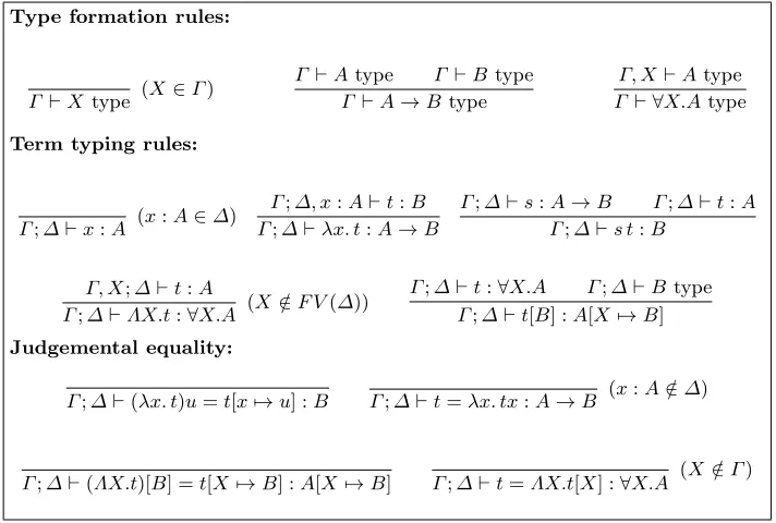
We now have the structure needed to define a 2-dimensional, proof-relevant model of System F. We recall the rules of System F in Fig. 1. Each type judgement
Γ `T type, with|Γ|=n, will be interpreted in the semantics as
JTK0:|1-Type|
n→1-Type
JTK1:|Rel|
n→Rel
JTK2:|2Rel|
n
→2Rel
by induction on type judgements with JTK1 over JTK0×JTK0, and JTK2 over JTK1×JTK1×JTK1×JTK1. This is similar to our previous work on bifibrational
Type formation rules:
Γ `X type (X ∈Γ)
Γ `Atype Γ `B type
Γ `A→B type
Γ, X `Atype
Γ ` ∀X.Atype
Term typing rules:
Γ;∆`x:A (x:A∈∆)
Γ;∆, x:A`t:B Γ;∆`λx. t:A→B
Γ;∆`s:A→B Γ;∆`t:A Γ;∆`s t:B
Γ, X;∆`t:A
Γ;∆`ΛX.t:∀X.A (X /∈F V(∆))
Γ;∆`t:∀X.A Γ;∆`B type
Γ;∆`t[B] :A[X 7→B]
Judgemental equality:
Γ;∆`(λx. t)u=t[x7→u] :B Γ;∆`t=λx. tx:A→B (x:A /∈∆)
[image:11.612.130.486.115.355.2]Γ;∆`(ΛX.t)[B] =t[X7→B] :A[X7→B] Γ;∆`t=ΛX.t[X] :∀X.A (X /∈Γ)
Fig. 1: Typing rules for System F
5.1 Interpretation of types
The full interpretation can be found in Fig. 2. For type variables and arrow types, we just use projections and exponentials at each level. Elements ofJ∀X.TK0A¯
consist of an ad-hoc polymorphic function f0, a proof f1 that f0 is suitably
uniform, and finally a (unique) proof (A0) that also the prooff1is parametric.
Similarly, elements of (J∀X.TK1R¯)(f, g) are proofsφthat are suitably parametric
in relation tof andg, both with respect to equalities (conditions A1.1 and A1.2) and connections (condition A1.3). We have not included uniformity also with respect to the “symmetric” connection since it is not needed for our applications, and we wish to keep the logical relation minimal.
Using Lemma 2 and function extensionality, we can characterise equality in the interpretation of∀-types in the following way (note that Id(
J∀X.TK2Q¯)f~
(~φ, ~ψ) is trivial by assumption, since (J∀X.TK2Q¯)f~is a proposition):
Lemma 21. For allf, g:J∀X.TK0A¯,
Id
J∀X.TK0A¯(f, g)
∼
={τ : (ΠA:1-Type)Id
JTK0( ¯A,A)(f0A, g0A)|
(∀R:Rel) (f1R, τ R0, g1R, τ R1)∈
Eq=(JTK1(Eq( ¯A), R))(f0R0, f0R1, g0R0, g0R1)}
JX0, . . . , Xn`XktypeKiY~ =Yk JS→TKiY~ =JSKiY~ ⇒iJTKiY~
J∀X.TK0A¯={f0 : (ΠA: 1-Type)JTK0( ¯A, A),
f1 : (ΠR:Rel)JTK1(Eq( ¯A), R)(f0R0, f0R1)|
(∀Q:2Rel) (f1Qr0, f1Q0r, f1Qr1, f1Q1r)∈
JTK2(Eq2( ¯A), Q)(f0Q00, f0Q10, f0Q01, f0Q11)} (A0)
(J∀X.TK1R¯)((f0, f1),(g0, g1)) ={φ: (ΠR:Rel)JTK1( ¯R, R)(f0R0, g0R1) | (∀Q:2Rel)
(f1Qr0, φQ0r, g1Qr1, φQ1r)∈
JTK2(Eqk( ¯R), Q)(f0Q00, f0Q10, g0Q01, g0Q11) (A1.1)
∧(φQr0, f1Q0r, φQr1, g1Q1r)∈
JTK2(Eq=( ¯R), Q)(f0Q00, f0Q10, g0Q01, g0Q11) (A1.2) ∧(f1Qr0, f1Q0r, φQr1, φQ1r)∈
JTK2(CR, Q¯ )(f0Q00, f0Q10, f0Q01, g0Q11)
} (A1.3)
(φ0, φ1, φ2, φ3)∈(J∀X.TK2Q¯)(f, g, h, l) iff
(∀Q:2Rel) (φ0Qr0, φ1Q0r, φ2Qr1, φ3Q1r)∈
JTK2( ¯Q, Q)(f0Q00, g0Q10, h0Q01, l0Q11)
Fig. 2: Interpretation of types
Theorem 22 (IEL). For every type judgementΓ `T type, we have
(i) an equivalenceΘT ,0:JTK1◦Eq∼=Eq◦JTK0,
(ii) an equivalenceΘT ,k:JTK2◦Eqk=∼Eqk◦JTK1 overΘT ,0,
(iii) an equivalenceΘT ,= :JTK2◦Eq==∼Eq=◦JTK1 overΘT ,0, and
(iv) an equivalenceΘT ,C:JTK2◦C∼=C◦JTK1 overΘT ,0. ut
Proof. We prove (i) for ∀-types, since it is useful in order to understand the logical relations in Fig. 2. We refer to the appendix for the rest of the proof. We define maps
for all f, g and show that they are inverses — this does not come for free, as in the proof-irrelevant setting, but will be considerably easier since we are considering 1-types only, and not arbitrary types. We first define Θ∀X.T ,0(ρ) := ϕ(λ(A: 1-Type). ρEq(A)), whereϕis part of the equivalence given by Lemma 21. The condition from Lemma 21 is satisfied by (A1.1) together with the induction hypothesis.
ForΘ∀−X.T ,1 0, we defineΘ∀−X.T ,1 0(τ) :=λR:Rel.tr(f1Eq(R0), τ R1)f1R. We need to
check that conditions (A1.1), (A1.2) and (A1.3) are satisfied — we verify (A1.1) in detail here, (A1.2) and (A1.3) follow analogously. LetQ:2Rel. By (A0), we have
(f1Qr0, f1Q0r, f1Qr1, f1Q1r)∈JTK2(Eq2( ¯A), Q)(f0Q00, f0Q10, f0Q01, f0Q11)
while we want to prove
(f1Qr0,tr(f1Eq(Q00), τ Q01)f1Q0r, g1Qr1,tr(f1Eq(Q10), τ Q11)f1Q1r)
∈JTK2(Eqk(Eq( ¯A)), Q)(f0Q00, f0Q10, g0Q01, g0Q11) .
SinceEqk(Eq( ¯A))∼=Eq2( ¯A), we only need to prove
p: (f0Q00, f0Q10, f0Q01, f0Q11)≡(f0Q00, f0Q10, g0Q01, g0Q11)
and
q:tr(p)(f1Qr0, f1Q0r, f1Qr1, f1Q1r)≡
(f1Qr0,tr(f1Eq(Q00), τ Q01)f1Q0r, g1Qr1,tr(f1Eq(Q10), τ Q11)f1Q1r) and transport alongpair=(p, q). We usep=pair=(f1Eq(Q00), f1Eq(Q10), τ Q01, τ Q11)
andq given by conditions (A1.1), (A1.3), (A0) for f1 and the condition from
Lemma 21.
We now check thatΘ∀X.T ,0◦Θ∀−X.T ,1 0=idandΘ
−1
∀X.T ,0◦Θ∀X.T ,0=id. One way
round
Θ∀X.T ,0(Θ∀−X.T ,1 0(τ))(A) =tr(f1Eq(A), τ A)f1Eq(A)≡(f1Eq(A))−1f1Eq(A)τ A≡τ A
by Lemma 1 as required. By definition we have Θ∀−X.T ,1 0(Θ∀X.T ,0(ρ))(R) =
tr(f1Eq(A), ρEq(B))f1R. Condition A1.3 implies that
(f1Eq(A), ρR, ρEq(B), f1R)∈JTK2(C(Eq( ¯A)),Eqk(R))(f0A, f0A, f0B, fB) and since C(Eq( ¯A))∼=Eqk(Eq( ¯A)), by the induction hypothesis (f1Eq(A), ρR, ρEq(B), f1R) are related in EqkJTK2(Eq( ¯A), R), i.e. tr(f1Eq(A), ρEq(B))f1R =
ρ(R) as required. ut
some seemingly arbitrary choices: we choose to only be uniform with respect to one connection, and we used the givenf1, not the giveng1, in order to construct
the isomorphism Θ∀−X.T ,1 0. The following lemma shows that these choices are actually irrelevant:
Lemma 23. For every type judgementΓ, X`T type and (f0, f1)∈J∀X.TK0A~, φ∈ J∀X.TK1(EqA~)(f, g), we have:
(i) For every relation R,tr(f1EqR0, φEqR1)f1R=φR.
(ii) For every relationR,
tr(f1EqR0, φEqR1)f1R=tr((φEqR0)−1,(g1EqR1)−1)g1R.
(iii) For every2-relation Q,
(φQr0, φQ0r, g1Qr1, g1Q1r)∈JTK2(C◦EqA, Q~ )(f0Q00, g0Q10, g0Q01, g0Q11). u t
Here, item (i) is a technical lemma, while item (ii) says that one can equally well useg1 asf1 in the proof of Theorem 22. Finally item (iii) shows that in certain
cases, the interpretation of terms of ∀-type are uniform also with respect to the other connection which is not explicitly mentioned in the logical relation for∀.
5.2 Interpretation of terms
We next show how to interpret terms. A term Γ;∆`t:T, with|Γ|=n, will be given a “standard” interpretation
JtK0A~:J∆K0A~→JTK0A ,~
for everyA~ : 1-Typen, a relational interpretation
(JtK0R~0,JtK0R~1,JtK1R~) :J∆K1R~ →JTK1R ,~
for everyR~ :Reln, and finally a 2-relational interpretation ((JtK0Q~−,JtK1Q~−),JtK2Q~) :J∆K2Q~ →JTK2Q~
for everyQ~ :2Reln, where we have written e.g.JtK0Q~− for the map ofI0-types
with components (JtK0Q~−)w=JtK0Q~w : J∆K0Q~w → JTK0Q~w and similarly for JtK1Q~−. At each level,∆=x1:T1, . . . , xm:Tmis interpreted as the product
Jx0:T0, . . . , xn:Tn`xk:TkKiX~ :=πk J∆, x:S`t:TKi=J∆`t:TKi◦π0
J∆`λx. t:S→TK0A~(γ) =λs.J∆, x:S`t:TK0A~(γ, s)
J∆`λx. t:S→TK1R~(γ) =λs0. λs1. λs.J∆, x:S`t:TK1R~((γ0, s0),(γ1, s1),(γ, s))
J∆`λx. t:S→TK2Q~((x, p), γ) =λ((x, p), γ).J∆, x:S`t:TK2Q~((x, x),(p, p))(γ, γ)
Jf tK0A~(γ) =JfK0A~(γ) (JtK0A~(γ))
Jf tK1R~(γ0, γ1, γ) =JfK1R~(γ0, γ1, γ,JtK0R~0(γ0),JtK0R~1(γ1),JtK1R~(γ0, γ1, γ))
Jf tK2Q~((x, p), γ) =JfK2Q~((x, p), γ,JtK0Q~i(x),JtK1Q~j(p),JtK2Q~((x, p), γ))
JΛX.tK0A~(γ) = (λA.J∆, X;∆`t:TK0(A, A~ )γ, λR.JtK1(Eq(A~), R)Θ∆,0(refl(γ)))
JΛX.tK1R~(γ0, γ1, γ) =λR.(JtK1(R, R~ ))(γ0, γ1, γ)
J∆`ΛX.t:∀X.TK2Q~((x, p), γ) =λQ.JtK2(Q, Q~ )((x, p), γ)
J∆`t[S] :T[S7→X]K0A~(γ) =fst(JtK0A~(γ))(JSK0A~)
Jt[S]K1R~(γ0, γ1, γ) =tr(ΘT ,0(snd(JtK0R~0γ0)Eq(JSK0R~0)))
−1
(JtK1R~(γ0, γ1, γ)(JSK1R~))
Jt[S]K2Q~((x, p), γ) =JtK2Q~((x, p), γ)(JSK2Q~)
Fig. 3: Interpretation of terms
The full interpretation is given in Fig. 3. Variables, term abstraction and term application are again given by projections and the exponential structure at each level. For type abstraction and type application, we use the same concepts at the meta-level, but we also have to prove that the resulting term satisfies the uniformity conditions (A0), (A1.1), (A1.2) and (A1.3). In addition, we have to put in a twist for the relational interpretation in order to validate the β- and
η-rules.
Lemma 24. The interpretation in Fig. 3 is well-defined.
Proof. The interpretation of Γ;∆ ` ΛX.t : ∀X.T is type-correct, since ∆ is weakened with respect toX inΓ, X;∆`t:T. The uniformity conditions (A0), (A1.1), (A1.2) and (A1.3) can all be proven using JtK2. ut
Theorem 25. The interpretation defined in Fig. 3 is sound, i.e. ifΓ;∆`s=t:
T, then there ispA¯:IdJTK0A¯(JsK0,JtK0)andqR¯:IdJTK1R¯(tr(pR¯0)(JsK1),JtK1). (We
automatically have tr(p, q)JsK2≡JtK2 by proof-irrelevance of 2-relations.) ut
the Reynolds relational interpretation of terms. In more detail: consider a term
Γ;∆`t:T with|Γ|=n. By construction, our model shows that ifR~ :Reln,a:
J∆K0R~0,b:J∆K0R~1andp:J∆K1R~(a, b), thenJtK1R p~ :JTK1R~(JtK0R~0a,JtK0R~1b),
i.e. JtK1R p~ is a proof that JtK0R~0 a and JtK0R~1 b are related at JTK1R~. This
is a proof-relevant version of Reynolds’ Abstraction Theorem. Furthermore, if
~
Q:2Reln, (a, b, c, d) :J∆K0Q~00×J∆K0Q~10×J∆K0Q~01×J∆K0Q~11and (p, q, r, s)∈ J∆K2Q~(a, b, c, d), then
(JtK1Q~r0p,JtK1Q~0rq,JtK1Q~r1r,JtK1Q~1rs)∈
JTK2Q~(JtK0Q~00a,JtK0Q~10b,JtK0Q~10c,JtK0Q~11d)
This is the Abstraction Theorem “one level up” for the proofsJtK1, which we will
put to use in the next section.
6
Theorems about Proofs for Free
In Phil Wadler’s famous ‘Theorems for free!’ [Wadler, 1989], the fact that para-metric transformations are always natural in the categorical sense is shown to have many useful and fascinating consequences. Among other things, it is shown that
JAK∼=J∀X.(A→X)→XK
for all types A — the categorically inclined reader will recognise this as an instance of the Yoneda Lemma (see e.g. Mac Lane [1998]) for the identity functor, if only we dared to consider the right hand side of the equation to consist of natural transformations only. And indeed, as Wadler shows (and Reynolds already knew [1983]), all System F termsJtK:J∀X.(A→X)→XKare natural by parametricity. Hence, in proof-irrelevant parametric models of System F, indeed
JAK∼=J∀X.(A→X)→XK.
In a more expressive theory such as (impredicative) Martin-L¨of Type Theory with proof-irrelevant identity types and function extensionality, we can go further even without a relational interpretation, as pointed out by Steve Awodey (personal communication). Taking inspiration from the Yoneda Lemma once again, we can show
A∼= (Σt: (ΠX:Set)(A→X)→X)isNat(t) (1) where
The above isomorphism (1) relied onAbeing a set, i.e. thatAhas no non-trivial higher structure. If we instead consider A: 1-Type, the isomorphism (1) fails; instead we have
A∼= (Σt: (ΠX :Set)(A→X)→X)(Σp:isNat(t))isCoh(p) (2) where
isCoh(p) := (ΠX, Y, Z : 1-Type)(Πf:X→Y)(Πg:Y →Z)
(p X Z(g◦f))≡(p Y Z g)?(p X Y f) expresses that the proofpis suitably coherent. Here (p Y Z g)?(p X Y f) is the operation that pastes the two proofsp X Y f andp Y Z g of diagrams commuting into a proof that the composite diagram commutes. Proof-irrelevant parametricity can not ensure this coherence condition, but as we will see, an extension of the usual naturality argument to proof-relevant parametricity will guarantee this extra uniformity of the proof as well.
6.1 Graph relations and graph 2-relations
Relations representing graphs of functions are key to many applications of parametricity.
Definition 26. Letf :A→Bin 1-Type. We define thegraphhfioff ashfi:= (A, B, λa. λb.IdB(f a, b)) :Rel. This extends to an action on commuting squares: if g:A0→B0,α:A→A0,β:B→B0 and p: (Πx:A)IdB0(g(α(a)), β(f(a))), then we definehα, βi= (α, β, λa. λb. λ(r:f a≡b). p(a)ap(β)(r)) :hfi → hgi.
Abstractly, we see thathfiis obtained fromEq(B) by “reindexing” along (f,id) and there is a morphismhf,idi:hfi →Eq(B); in particular, we recoverEq(B) ashidBi. Just likeEqis full and faithful, so ish−i: 1-Type→→Rel:
Lemma 27. For allf :A→B,g:A0→B0,
(hfi ⇒ hgi)∼= (Σα:A→A0)(Σβ:B→B0)IdA→B0(g◦α, β◦f) .
u t
The main tool for deriving consequences of parametricity is the Graph Lemma, which relates the graph of the action of a functor on a morphism with its relational action on the graph of the morphism.
Theorem 28. LetF0 :1-Type→1-Type and F1: Rel→Rel over F0 be
func-torial. If F1(Eq(A)) ∼=Eq(F0A) for all A, then for any f : A → B, there are
Note that in our proof-relevant setting, this theorem does not construct an equivalencehF0fi ∼=F1hfi. Instead, we only have a logical equivalence, i.e. maps
in both directions, and that seems to be enough for all known consequences of parametricity. (In a proof-irrelevant setting, the constructed logical equivalence would automatically be an equivalence.)
Next, we consider also graph relations. Since we have multiple “equality 2-relations”, one could expect also multiple graph 2-relations, but for the application we have in mind, one suffices. Given functionsf,g,l andh, we write(f, g, l, h) for the 1-type of proofs that the square
A f //
h B g C
l //D
commutes, i.e.(f, g, l, h) = (Πx:A)IdD(g(f x), l(hx)). We define the 1-type of commuting squares by
(1-Type→)→:= (Σf :A→B)(Σg:B→D)(Σl:C→D)(Σh:A→C)(f, g, l, h) A morphism (f, g, l, h, p)→(f0, g0, l0, h0, p0) in (1-Type→)→ consists of four mor-phismsα:A→A0, β :B →B0,γ :C→C0 andδ:D →D0, and four proofs
q:(α, h0, γ, h),q0 :(β, f0, δ, g),r:(γ, l0, δ, l) andr0 :(α, f0, β, f) such that they form a “commuting cube”
B β //
g B0 g0 A
f ??
α // h
A0
f0 ??
h0
D
δ //D
0
C γ //
l ??
C0 l
0
?
?
i.e. such that p ? q ? r≡p0? q0? r0, wherep ? q ? r andp0? q0? r0 are pastings of the squares that proves that both ways from one corner of the cube to the opposite one commutes. The 2-graphh i2: (1-Type→)→→2Relis defined by hf, g, h, l, pi2:= (hfi,hgi,hhi,hli, λ(a, b, c, d). λ(q, r, s, t). w(a)ap(g)pq≡ap(l)sr)
Lemma 29. h−i2 is full and faithful in the sense that
(hf, g, h, l, pi2→2Relhf0, g0, h0, l0, p0i2)∼= (f, g, h, l, p)→(1-Type→)→(f0, g0, h0, l0, p0)
u t
This lemma can be used to prove a 2-relational version of the Graph Lemma: Theorem 30 (2-relational Graph Lemma). LetF2 :2Rel →2Rel be
func-torial, and over(F0, F1) whereF0 andF1 are as in Theorem 28. If F2(EqR)∼=
Eq(F1R)for allR, then for any(f, g, h, l, p)in(1-Type→)→, there are morphisms φ2:hF0f, F0g, F0h, F0l,ap(F0)pi2→F2hf, g, h, l, pi2 andψ2:F2hf, g, h, l, pi2→ hF0f, F0g, F0h, F0l,ap(F0)piin2Relover(φ, φ)and(ψ, ψ)from Theorem 28. ut
6.2 Coherent proofs of naturality
Let us now apply the tools we have developed to the question of the coherence of the naturality proofs from parametricity. We first recall the standard theorem that holds also with proof-irrelevant parametricity:
Theorem 31 (Parametric terms are natural).LetF(X)andG(X)be func-torial type expressions in the free type variableX in some type context Γ. Every termΓ;− `t:∀X.F(X)→G(X)gives rise to a natural transformationJFK0→ JGK0, i.e. iff :A→B then there isnat(f) :Id(JGK0(f)◦JtK0A,JtK0B◦JFK0(f)).
Proof. We constructnat(f) using the relational interpretation oft: By construc-tion,JtK1hfi:JFK1(hfi)→JGK1(hfi), hence using Theorem 28,
ψG,f◦JtK1hfi ◦φF,f : (Πxy)hJFK0fi(x, y)→ hJGK0fi(JtK0Ax,JtK0B y)
and sincerefl:hJFK0fi(a,(JFK0f)a) for eacha:JFK0A, we can definenat(f) :=
ext(λa.(ψG,f◦JtK1hfi ◦φF,f)a((JFK0f)a)refl). ut
In order for (JtK0,nat) to lie in the image of the isomorphism (2), we also need the
naturality proofs to be coherent. But thanks to the 2-relational interpretation, we can show that they are:
Theorem 32 (Naturality proofs are coherent). Let F, G and t be as in Theorem 31. The proof nat:isNat(JtK0)is coherent, i.e. for all f :A→B and
g:B →C, there is a proof coh(f, g) :Id(nat(g◦f),nat(g)?nat(f)).
Proof. We construct coh(f, g) using the 2-relational interpretation of t. By construction, JtK2hf, g, g◦f,id,refli2 : JFK2hf, g, g◦f,id,refli2 →JGK2hf, g, g◦ f,id,refli2, hence using Theorem 30,
φ2◦JtK2hf, g, g◦f,id,refli2◦ψ2:
(Π(¯x,r¯)) ¯r∈ hF0f, F0g, F0(g◦f),id,ap(F0)pi2x¯
→(JtK1r¯)∈ hG0f, G0g, G0(g◦f),id,ap(G0)pi2(JtK0x¯)
We define
coh(f, g) :=ext(λa.(φ2◦JtK2hf, g, g◦f,id,refli2◦ψ2) (a,(F0f)a, F0(g◦f)a, a)refl)~
— this works, sinceφ2andψ2are over (φ, φ) and (ψ, ψ) respectively, sincenat(h)
is defined to be (φ◦JtK1 ◦ψ)refl, and since the 2-relation hG0f, G0g, G0(g◦ f),id,ap(G0)pi2 exactly says that pasting the two diagrams produces the third
in this case. ut
7
Conclusions and future work
In this paper, we tackled the concrete problem of transporting Reynolds’ theory of relational parametricity to a proof-relevant setting. This is non-trivial as one must modify Reynolds’ uniformity predicate on polymorphic functions so that it itself becomes parametric. Implementing this intuition has significant mathematical ramifications: an extra layer of 2-dimensional relations is needed to formalise the idea of two proofs being related to each other. Further, there are a variety of choices to be made as to what face maps and degeneracies to use between proof-relevant relations and 2-relations. Having made these choices, we showed that the key theorems of parametricity, namely the identity extension lemma and the fundamental theorem of logical relations hold. Finally, we explored how a standard consequence of relational parametricty — namely the fact that parametricity implies naturality — also holds in the proof-relevant setting. This work complements the more proof-theoretic work oninternal parametricity in proof-relevant frameworks [Bernardy et al., 2015, 2012; Polonsky, 2015]. Relevant is also the work on parametricity for dependent types in general [Atkey et al., 2014; Krishnaswami and Dreyer, 2013], assuming proof-irrelevance.
In terms of future work, we are extending the results of this paper to arbitrary dimensions. We have a candidate definition of higher-dimensional relations, the requisite face maps and degeneracies and we have proven the Identity Extension Lemma. What remains to do is to fully investigate the consequences. For instance, what form of higher dimensional initial algebra theorem can be proved with higher dimensional parametricity? More generally, we need to compare the methods, structures and results of higher dimensional parametricity with (where possible) Homotopy Type Theory and in particular its cubical sets model [Bezem et al., 2014], which shares many striking similarities. Finally, once the theoretical frame-work is settled, we will want to implement it and then use that implementation in formal proof.
References
Atkey, R.: Relational parametricity for higher kinds. In: C´egielski, P., Durand, A. (eds.) CSL 2012. LIPIcs, vol. 16, pp. 46–61. Schloss Dagstuhl – Leibniz-Zentrum
f¨ur Informatik (2012)
Atkey, R., Ghani, N., Johann, P.: A relationally parametric model of dependent type theory. In: POPL. pp. 503–515. ACM (2014)
Bernardy, J.P., Coquand, T., Moulin, G.: A presheaf model of parametric type theory. In: Ghica, D.R. (ed.) MFPS. pp. 17–33. ENTCS, Elsevier (2015) Bernardy, J.P., Jansson, P., Paterson, R.: Proofs for free. Journal of Functional
Programming 22, 107–152 (2012)
Bezem, M., Coquand, T., Huber, S.: A model of type theory in cubical sets. In: Types for Proofs and Programs (TYPES 2013). Leibniz International Proceedings in Informatics, vol. 26, pp. 107–128. Schloss Dagstuhl–Leibniz-Zentrum f¨ur Informatik (2014)
Brown, R., Higgins, P.J.: On the algebra of cubes. Journal of Pure and Applied Algebra 21(3), 233 – 260 (1981)
Brown, R., Higgins, P.J., Sivera, R.: Nonabelian Algebraic Topology: Filtered spaces, crossed complexes, cubical homotopy groupoids, EMS Tracts in Mathe-matics, vol. 15. European Mathematical Society Publishing House (2011) Coquand, T., Huet, G.: The Calculus of Constructions. Information and
Compu-tation 76, 95–120 (1988)
Dunphy, B., Reddy, U.: Parametric limits. In: LICS. pp. 242–251 (2004) Garner, R.: Two-dimensional models of type theory. Mathematical Structures in
Computer Science 19(04), 687–736 (2009)
Ghani, N., Johann, P., Nordvall Forsberg, F., Orsanigo, F., Revell, T.: Bifibra-tional functorial semantics of parametric polymorphism. In: Ghica, D.R. (ed.) MFPS. pp. 67–83. ENTCS, Elsevier (2015a)
Ghani, N., Nordvall Forsberg, F., Orsanigo, F.: Parametric polymorphism — universally. In: de Paiva, V., de Queiroz, R., Moss, L.S., Leivant, D., de Oliveira, A.G. (eds.) WoLLIC. LNCS, vol. 9160, pp. 81–92. Springer (2015b)
Grandis, M.: The role of symmetries in cubical sets and cubical categories (on weak cubical categories, I). Cah. Topol. Gom. Diff. Catg. 50(2), 102–143 (2009) Krishnaswami, N.R., Dreyer, D.: Internalizing relational parametricity in the
extensional calculus of constructions. In: CSL. pp. 432–451 (2013)
Mac Lane, S.: Categories for the working mathematician, vol. 5. Springer (1998) Martin-L¨of, P.: An intuitionistic theory of types (1972), published in Twenty-Five
Years of Constructive Type Theory
O’Hearn, P.W., Tennent, R.D.: Parametricity and local variables. Journal of the ACM 42(3), 658–709 (1995)
Polonsky, A.: Extensionality of lambda-*. In: Herbelin, H., Letouzey, P., Sozeau, M. (eds.) 20th International Conference on Types for Proofs and Programs (TYPES 2014). Leibniz International Proceedings in Informatics (LIPIcs), vol. 39, pp. 221–250. Schloss Dagstuhl–Leibniz-Zentrum f¨ur
Reynolds, J.: Types, abstraction and parametric polymorphism. In: Mason, R.E.A. (ed.) Information Processing 83. pp. 513–523 (1983)
Robinson, E., Rosolini, G.: Reflexive graphs and parametric polymorphism. In: LICS. pp. 364–371 (1994)
Strachey, C.: Fundamental concepts in programming languages. Higher Order Symbolic Computation 13(1-2), 11–49 (2000)
The Univalent Foundations Program: Homotopy Type Theory: Univalent Foun-dations of Mathematics. http://homotopytypetheory.org/book(2013) Voevodsky, V.: The equivalence axiom and univalent models of type theory. Talk
at CMU on February 4, 2010 (2010),http://arxiv.org/abs/1402.5556 Wadler, P.: Theorems for free! In: FPCA. pp. 347–359 (1989)
Wadler, P.: The Girard-Reynolds isomorphism (second edition). Theoretical Computer Science 375(1-3), 201–226 (2007)
A
Proofs from Section 5
Proof (of Theorem 22). The proof is done by induction on type judgements. For type variables, all statements are trivial. For arrow types, this is Propositions 8 and 20.
It remains to prove (ii), (iii) and (iv) for ∀-types. In this case we only need to produce maps in both directions — they will automatically compose to the identity by proof-irrelevance of 2-relations. The structure of the proof is the same for all of the three points.
For (ii) consider (τ0, ρ0, τ1, ρ1)∈Eqk(J∀X.TK1R¯)(f, g, h, l). We want to show that
(Ψ(τ0), ρ0, Ψ(τ1), ρ1)∈J∀X.TK2Eqk( ¯R)(f, g, h, l), i.e. that for every 2-relationQ, (Ψ(τ0)Qr0, ρ0Q0r, Ψ(τ1)Qr1, ρ1Q1r)∈JTK2(Eqk( ¯R), Q)(f0Q00, g0Q10, h0Q01, l0Q11).
By condition A1.1, we have
(f1Qr0, ρ0Q1r, f1Qr1, ρ0Q0r)∈JTK2(Eqk( ¯R), Q)(f0Q00, f0Q10, h0Q01, h0Q11)
and using the equalities (f1EqQ00, τ0EqQ10, h1EqQ01, τ1EqQ11), we can show
(f0Q00, g0Q10, h0Q01, l0Q11, Ψ(τ0)Qr0, ρ0Q0r, Ψ(τ1)Qr1, ρ1Q1r)
≡(f0Q00, f0Q10, h0Q01, h0Q11, f1Qr0, ρ0Q1r, f1Qr1, ρ0Q0r) We now transport across this equality to finish the argument.
Finally, in the other direction, if (ρ0, ρ1, ρ2, ρ3)∈J∀X.TK2Eqk( ¯R)(f, g, h, l), then
(Θ(ρ0), ρ1, Θ(ρ2), ρ3)∈Eqk(J∀X.TK1R¯)(f, g, h, l) by straightforward calculation
and the definition ofJ∀X.TK2.
The last case (iv) is more complicated. Consider (τ0, τ1, ρ0, ρ1)∈C(J∀X.TK1R¯)(f, g, h, l).
We want to show that (Ψ(τ0), Ψ(τ1), ρ0, ρ1)∈J∀X.TK2C( ¯R)(f, g, h, l), i.e. that
for every 2-relationQ,
(Ψ(τ0)Qr0, Ψ(τ1)Q0r, ρ0Qr1, ρ1Q1r)∈JTK2(C( ¯R), Q)(f0Q00, g0Q10, h0Q01, l0Q11) .
By condition A1.3, we have
(h1Qr0, h1Q1r, ρ0Qr1, ρ0Q0r)∈JTK2(CR, Q¯ )(h0Q00, h0Q10, h0Q01, l0Q11)
and using the equalities
((τ1Q00)−1)f1EqQ00,(τ1EqQ10)−1τ0Q10,(h1EqQ01)−1h1EqQ01,refl),
we can show
(f0Q00, g0Q10, h0Q01, l0Q11, Ψ(τ0)Qr0, Ψ(τ1)Q0r, ρ0Qr1, ρ1Q1r)
≡(h0Q00, h0Q10, h0Q01, l0Q11, h1Qr0, h1Q1r, ρ0Qr1, ρ0Q0r) We can now transport across this equality to finish the argument. This re-quires the use of Lemmas 23 (i) and (ii), and the fact that (τ0, τ1, ρ0, ρ1) ∈
C(J∀X.TK1R¯)(f, g, h, l).
Finally, In the other direction, if (ρ0, ρ1, ρ2, ρ3)∈J∀X.TK2C( ¯R)(f, g, h, l), then
(Θ(ρ0), Θ(ρ1), ρ2, ρ3) ∈ C(J∀X.TK1R¯)(f, g, h, l) by straightforward calculation
and the definition ofJ∀X.TK2. ut
Proof (of Lemma 23).
(i) Since
(f1R, f1EqR0, f1R, f1EqR1)∈JTK2(C◦Eq(A~),Eq=(R))(f0R0, f0R1, g0R0, g0R1)
andJTK2(C◦Eq(A~),Eq=(R)) =JTK2(Eq=◦Eq(A~),Eq=(R))=∼Eq=(JTK1(EqA, R~ )),
by Theorem 22(iii), the thesis follows. (ii) By assumption,
(f1R, φEqR0, g1R, φEqR1)∈JTK2(Eq=EqA,~ Eq=R)(f0R0, f1R1, g0R0, g0R1).
By Theorem 22(iii),JTK2(Eq=EqA,~ Eq=R)∼=Eq=(JTK1(EqA, R~ )), hence we
have tr((φEqR0)−1,(g1EqR1)−1)g1R = tr(f1EqR0, φEqR1)f1R. If we now
transport (f1R, φEqR0, g1R, φEqR1) along the equality proof ((f1EqR0)−1,
(f1EqR1)−1,(φEqR0)−1,(g0EqR1)−1), the result follows.
(iii) By assumption,
(g1Qr0, g1Q0r, g1Qr1, g1Q1r)∈JTK2(Eq2A, Q~ )(g0Q00, g0Q10, g0Q01, g0Q11)
We can transport (g1Qr0, g1Q0r, g1Qr1, g1Q1r) along the equality ((φEqQ00)−1,
Proof (of Theorem 25). We need to check that the β- and η-rules for both term and type abstraction are respected. For term abstraction, this follows from Lemmas 13 and 16.
We next consider theη-rule for type abstraction. LetΓ;∆`t:∀X.Tbe given. Let
JtK0Aγ~ = (f0, f1). ShowingJΛX.t[X]K0≡JtK0 means givingp0:Id(λA.f0A, f0)
andp1:Id(λR.(tr(p0(snd((JtK0Aγ¯ )Eq(R0))))
−1(
JtK1Eq( ¯A)Θ∆,0(refl(γ))R)),snd(JtK0Aγ¯ )).
Forp0, we choosep0=refl. Note that
(JtK1Eq( ¯A)Θ∆,0(refl(γ))R)) =Θ∆,0(refl(JtK0Aγ~ ))R=
tr(f1Eq(R0),refl)f1R
under the equivalence with respect to τ=refl, and
tr(refl(snd((JtK0Aγ¯ )Eq(R0))))−1=tr(f1Eq(R0),refl)−1.
In this way we can conclude
tr(f1Eq(R0),refl)−1(Θ∆,0(refl(JtK0Aγ~ ))R) =tr(f1Eq(R0),refl)
−1tr(f
1Eq(R0),refl)f1R
=f1R.
Similarly, things are exactly lined up to maketr(pair=(p0, p1))(JΛX.t[X]K1)≡JtK1
trivial.
For theβ-rule, considerΓ, X`t:T. We can usepA¯= (JtK1Eq(A,~ JSK0A~)Θ∆,0(refl(γ)))
−1