A Signal processing approach for preprocessing and 3d analysis of airborne small-footprint full waveform lidar data

(1)

Rochester Institute of Technology

RIT Scholar Works

Theses Thesis/Dissertation Collections

8-14-2012

A Signal processing approach for preprocessing and

3d analysis of airborne small-footprint full

waveform lidar data

Jiaying Wu

Follow this and additional works at:http://scholarworks.rit.edu/theses

This Dissertation is brought to you for free and open access by the Thesis/Dissertation Collections at RIT Scholar Works. It has been accepted for inclusion in Theses by an authorized administrator of RIT Scholar Works. For more information, please [email protected].

Recommended Citation

(2)

A SIGNAL PROCESSING APPROACH FOR PREPROCESSING AND 3D ANALYSIS OF

AIRBORNE SMALL-FOOTPRINT FULL WAVEFORM LIDAR DATA

by

Jiaying Wu

B.S. University of Shanghai for Science and Technology

(2006)

A dissertation submitted in partial fulfillment of requirements for the degree of Ph.D.

in the Chester F. Carlson Center for Imaging Science of the College of Science

Rochester Institute of Technology

August 14, 2012

Signature of author ____________________________________________________

Accepted by _________________________________________________________

(3)

CHESTER F. CARLSON CENTER FOR IMAGING SCIENCE

COLLEGE OF SCIENCE

ROCHESTER INSTITUTE OF TECHNOLOGY ROCHESTER, NEW YORK

CERTIFICATE OF APPROVAL

Ph.D. DEGREE DISSERTATION

The Ph.D. Degree Dissertation of Jiaying Wu has been examined and approved by the dissertation committee as satisfactory for the

dissertation requirement for the Ph.D. degree in Imaging Science

______________________________________________________ Dr. Jan van Aardt, Thesis Advisor Date

______________________________________________________ Dr. John Kerekes Date

______________________________________________________ Dr. Harvey Rhody Date

______________________________________________________ Dr. Vinny Amuso Date

(4)

DISSERTATION RELEASE PERMISSION ROCHESTER INSTITUTE OF TECHNOLOGY

COLLEGE OF SCIENCE CHESTER F. CARLSON CENTER FOR IMAGING SCIENCE

Title of Dissertation:

A Signal Processing Approach For Preprocessing and 3D Analysis of Airborne Small-Footprint Full Waveform LiDAR Data

I, Jiaying Wu, hereby grant permission to Wallace Memorial Library of R.I.T. to reproduce my thesis in whole or in part. Any reproduction will not be for commercial use or profit.

Signature: ____________________

(5)

A SIGNAL PROCESSING APPROACH FOR PREPROCESSING AND 3D ANALYSIS OF

AIRBORNE SMALL-FOOTPRINT FULL WAVEFORM LIDAR DATA

by Jiaying Wu

A dissertation submitted in fulfillment of requirements for the degree of Ph.D. in the Chester F. Carlson Center for Imaging

Science

of the College of Science Rochester Institute of Technology

Abstract

The extraction of structural object metrics from a next generation remote sensing modality, namely waveform light detection and ranging (LiDAR), has garnered increasing interest from the remote sensing research community. However, a number of challenges need to be addressed before structural or 3D vegetation modeling can be accomplished. These include proper processing of complex, often off-nadir waveform signals, extraction of relevant waveform parameters that relate to vegetation structure, and from a quantitative modeling perspective, 3D rendering of a vegetation object from LiDAR waveforms. Three corresponding, broad research objectives therefore were addressed in this dissertation.

(6)

to recover the temporal signal resolution, and resulted in improved waveform-based vegetation biomass estimation.

Secondly, a model for savanna vegetation biomass was derived using the resultant processed waveform data and by decoding the waveform in terms of feature metrics for woody and herbaceous biomass estimation. The results confirmed that small-footprint waveform LiDAR data have significant potential in the case of this application.

(7)

ACKNOWLEDGEMENTS

First of all I want to thank my advisor Dr. Jan van Aardt. It has been an honor to be his first Ph.D. student. It would not have been possible to write this doctoral thesis without his excellent guidance and support on both an academic and a personal level. I appreciate all his contributions in terms of time, ideas, and funding to make my Ph.D. experience productive and stimulating.

I would also like to acknowledge the financial, academic, and technical support of my department, the Chester F. Carlson Center for Imaging Science, Rochester Institute of Technology towards completing my Ph.D. research, travel, publishing, etc.

This research would not have been possible without the support from Carnegie Institution for Science, Stanford, CA. I am most grateful to my thesis co-advisor, Dr. Gregory P. Asner, for his inputs to the vegetation biomass study, and his extraordinary contribution in building up the Carnegie Airborne Observatory, which is funded by the W.M. Keck Foundation and William Hearst III. Dr. Asner also hosted me at their lab in Stanford, CA for the academic collaboration twice during my Ph.D study. Together with Mr. Ty Kennedy-Bowdoin, Mr. Dave Knapp and Mr. Aravindh Balaji, he provided the airborne waveform LiDAR data and technical support, for which I am extremely grateful. Also, my thanks goes to Dr. Konrad Wessels, Dr. Renaud Mathieu (Council for Scientific and Industrial Research), and Dr. Barend Erasmus (University of the Witwatersrand) for their field data collection support.

I would also like to thank Dr. Michael Long (RIT) for his inputs during discussions on statistical analysis, Dr. Harvey Rhody for his excellent instruction on signal processing, and Dr. John Kerekes for his advising on image processing algorithms. I want to thank my classmates, also friends, David Kelbe, Paul Romanczyk, Joseph McGlinchy, and Diane Sarrazin, and Dr. Kerry Cawse-Nicholson in our waveform LiDAR study group. I feel so lucky to work with such smart and kind people. Most of my inspirations originate from our team work, discussions, and brainstorming, where we share ideas with each other.

(8)

List of Figures

1.1 An overview of the research objectives ……….. 3

1.2 Illustration of the discrete return LiDAR signal ………...…….. 7

1.3 Illustration of the full-waveform LiDAR signal ………... 9

1.4 An example of 3D reconstruction of tree branches based on Gorte and Pfeifer’s [14] voxel approach ………..………... 18

1.5 Probabilistic 3D reconstruction of branches, proposed by Binney and Sukhatme . 18 1.6 3D tree reconstruction proposed by Cote et al. [35] ………….……...……... 19

1.7 (a) Typical bimodal waveform. (b) Relationship between field measurements and estimates of maximum canopy height from waveform parameters [36] …... 20

1.8 Metrics derived from synthetic large-footprint LiDAR waveforms [41] …... 22

2.1 A flowchart of the waveform LiDAR preprocessing chain ………... 24

2.2 The study area and associated land use gradient in South Africa …………... 25

2.3 CAO Alpha system with the ALTM 3100 waveform LiDAR system ……... 26

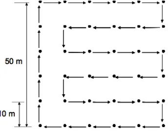
2.4 Site-level sampling design with 36 plots/site ………... 26

2.5 An example of a virtual scene for generating simulated waveform LiDAR … 27

2.6 Histogram of the zenith (a) and azimuth (b) angle distribution based on real waveform LiDAR data collected by CAO ……….... 29

2.7 Illustration of the waveform noise filtering: (a) Real (raw) waveform data collected by the Carnegie Airborne Observatory system and (b) the smoothed waveform following frequency-based noise filtering. Note: a negative noise level shift of 11 units was applied to the raw signal first to avoid the potential frequency leakage caused by the sharp edge at the inflection point (signal on/off) …………... 31

2.8 A typical frequency representation of a waveform signal. A cut-off frequency threshold of 20GHz was selected based on visual assessment of filtering results; any frequency component above 20GHz was attributed to noise and set to zero. Simulated 3D trees used for waveform simulation and deconvolution assessment …………..………..………..……... 31

(11)

2.11 An example of a 3D grass patch (the different herbaceous biomass levels were simulated by scaling the relative size of the grass facet while keeping the patch area

of 100m2_{constant) ………...………... 38}

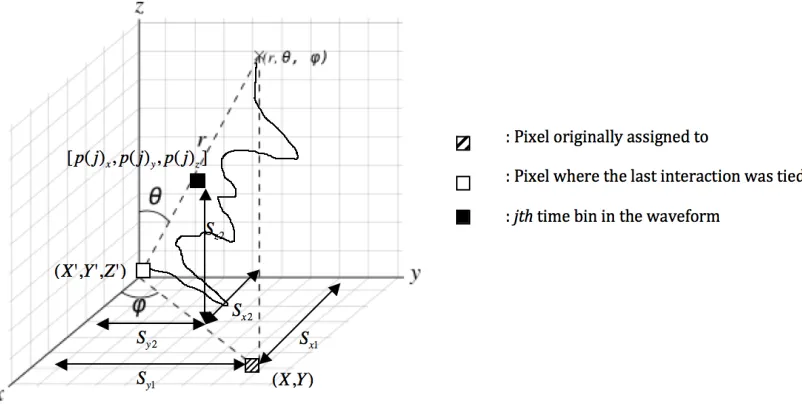
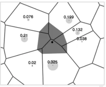
2.12 Illustration of the waveform registration principles ………... 40 2.13 Illustration of a waveform angular vector map based on CAO data collected in a

savanna area, South Africa; note the displacement of less than one pixel size (blue) and displacement larger than one pixel size (red). The direction of the vector indicates the azimuth angle and the length is equal the level of waveform displacement (rprojection) in this angular vector map ………..………... 41

2.14 An illustration of the gridding process for registered waveform time bins, where (a) shows an example of an off-nadir waveform, (b) shows the vertical sampling plane, and (c) represents the time bins associated with the same absolute height above sea level ………..…………... 43 2.15 Natural neighbor interpolation. Figure taken from the Wikipedia entry on natural neighbor interpolation [52] ………..………... 43 2.16 Illustration of spectral angle, as calculated using the spectral angle mapper (SAM) approach. Note: only three bands are shown in this example; this metric can be applied to multi-dimensional data ………...….……... 45 2.17 An illustration of the deconvolved waveforms for an outgoing pulse width of 8ns: RL (a), WF (b), and NNLA (c) ……….………....………... 49 2.18 A 3D representation of the waveform LiDAR for tree 6 and all deconvolution approaches at 8ns and 16ns outgoing pulse widths ………...………... 50 2.19 Results of the RMSE comparison for outgoing pulse width 8ns (a) and 16ns (b)

………...………..……….………... 52 2.20 Point clouds extracted from the local peaks of the waveforms (Tree 5). The point

(12)

2.22 Simulated waveforms from grass patches: (a) before deconvolution, and (b) after deconvolution. Herbaceous biomass ratios from patch 1 to 5 were 0.23_{: 0.4}3_{: 0.6}3_:

0.83_{: 1. The plots are based on the RL deconvolution algorithm with an outgoing}

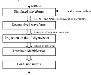
pulse width equal to 8ns ……….………...…... 56 2.23 Plot of the normalized cumulative sum of the eigenvalues for the simulated

waveforms from grass patches; (b) Eigenvectors associated with the four largest eigenvalues in descending order ……….………...…... 57 2.24 (a) Projection on the 1st eigenvector vs. projection on the 2nd eigenvector. (b)

Histogram of the projection on the 1st eigenvector ………….………....…... 58 2.25 Comparison of the classification accuracy for no deconvolution and the three

deconvolution algorithms in question ……….…………...…... 59 2.26 A 3D representation of the voxelized waveforms. (a): Raw waveform (8ns pulse width, zenith=5°). (b): Truth waveform (2ns pulse width). (c): Fully processed waveform …...…... 61 2.27 Stepwise evaluation of the processing chain performance; 4ns (a), 8ns (b) and 16ns

(c) outgoing pulse widths. Raw (Raw data), Nos (Noise Reduction), Dev (Deconvolution), Reg (Registration), Ang (Angular Rectification) …....…... 64 2.28 An illustration of the impact that waveform registration and angular rectification have on the processing of waveform LiDAR signals. The truth waveform (a) is compared to the reconstructed waveform (b) after registration and angular rectification. The various off-nadir waveforms are shown before processing for azimuths 0°, 90°, 180°, and 270°, and a zenith of 10° for all (c,d,e,f) …... 65 2.29 An example of a waveform LiDAR metric used for woody biomass modeling and

the impact of processing steps: (clock-wise, from top left) a panchromatic image of a site within the study area (a), 10-90% duration metric (b), after threshold removal and de-noising (c), deconvolution (d), ground registration and angular rectification (e) ………...…... 67 2.30 Model R2 as a function of the waveform processing steps (a). There is a slight

(13)

2.31 The distribution of allometry-estimated (field-based) woody biomass (kg) for the

individual trees used in this study……..…...…... 68

3.1 A graphical representation of the metrics extracted from each LiDAR waveform 72 3.2 3D volumetric waveform visualization at the individual tree level. The presentations show x,y,z coordinates, with waveform intensity color-coded from cool (blue; low) to warm (red; high) ………...…... 73

3.3 An example of a histogram showing the crown thickness distribution, derived from multiple LiDAR waveforms (0.56 m), for an individual tree canopy ….…... 74

3.4 Modeling the herbaceous biomass by Gaussian decomposition; it was hypothesized that the complexity of the herbaceous layer is correlated to the multiple scattering component …...…... 75

3.5 (a) Height, (b) foliar biomass, and (c) woody biomass estimation using waveform LiDAR metrics ………....…... 78

3.6 Herbaceous biomass estimation using waveform LiDAR-derived metrics …. 80

4.1 (a) 3D tree branches input and associated point clouds extracted from simulated waveform data (b) ………....…... 84

4.2 An illustration of the DBSCAN algorithm that shows the arbitrary nature of cluster shapes [68] ………...…... 86

4.3 1st order branch characteristics in terms of L and Ɵ…...………...…... 88

4.4 An example of how a first order branch can be reconnected to the stem …... 89

4.5 Definition of tree azimuth and zenith angle ……….…... 90

4.6 Branch representation using waveform LiDAR data with different intensity thresholds. e.g., all the point clouds intensity are larger >3 while T=3 (this was done based on tree #2) ………..………...…... 91

4.7 A graphical representation of the optimal threshold for clustering .………... 92

4.8 Results of DBSCAN clustering based on optimal threshold; Different cluster is distinguished by color ….………...…... 93

(14)

leaf-4.11 (a) Leaf-off tree input. (b) Final reconstruction result of the branches for the leaf-off

scenario …...……... 94

4.12 (a) Raw point clouds extract from the waveform, (b) after applying optimal intensity threshold …...…... 95

4.13 Stem reconstruction for leaf-on condition. (a) Leaf-on tree input, (b) reconstructed stem from a side view, (c) reconstructed stem from a top view …...…... 95

4.14 1st order branches approximated by cylinders from clusters for a tree model in the leaf-on scenario ……….……...…... 96

4.15 (a) Leaf-on tree input. (b) Final reconstruction result of the branches for the leaf-on scenario.………..…... 97

4.16 Branch reconstruction characterization for leaf-off (a) and leaf-on (b) scenario . 98 4.17 Branch reconstruction results (a) original 3D tree model (leaf-on), (b) original 3D tree model (leaf-off), (c) reconstructed tree branches using waveform simulated from leaf-on tree, (d) quantitative results of 2ns and 4ns pulse width branch reconstruction (leaf-on) accuracy by comparing to the truth data (2ns leaf-off). Note: Azimuth Angle (AA), Title Angle (TA), Normalized Branch Length (BL) 99 A.1 Workflow of waveform LiDAR simulation using DIRSIG ……….…..…... 107

A.2 Outgoing pulses used by CAO system (ALTM 3100EA) ………..….... 109

A.3 LiDAR_tools main user interface ……….……..….... 111

A.4 LiDAR_tools data viewer ……….……..….... 112

A.5 Waveform LiDAR data viewer ……….……..….... 112

(15)

List of Tables

1.1 Basic LiDAR formula ………...……….. 5

1.2 Specification of six waveform LiDAR systems ……….. 9

2.1 A description of the LiDAR system configuration ………..…... 29

2.2 Specifications of the 3D virtual tress used for waveform simulation…...…... 35

2.3 Statistics of the peak detection results ……….…... 54

2.4 Illustration of confusion matrix used for assessing the accuracy of herbaceous biomass classification (based on RL) …...…... 59

3.1 Correlation coefficients between field data (blue) and waveform-derived metrics (yellow) (D= diameter measured above basal swelling; H=measured height) .. 77

3.2 Correlation coefficients between field data and waveform-derived feature metrics for herbaceous biomass estimation ………..…... 80

4.1 Quantitative comparison of the branch reconstruction for leaf-off and leaf-on condition, Δ represents difference for each metric …………... 98

(16)

Chapter 1: Introduction

The assessment and monitoring of ecosystem change, such as biomass accumulation, typically involve extensive field data collection. Such data collection typically includes sampling of parameters such as foliar area, stem diameter, tree height, and volume or woody biomass. The acquisition of these data can be expensive and time consuming, while leaving the user with a relatively crude approach when modeling intricate dependent variables, such as woody and foliar biomass, volume, etc. In the recent decades, the application of waveform Light Detection and Ranging (LiDAR) [1-3] remote sensing technology in forestry has become an effective approach to facilitate in-field measurement and vegetation structure characterization, especially due to its unique capability of providing the three-dimensional (3D) information. However, the waveform LiDAR signal still presents significant challenges to implementers.

Firstly, since waveform LiDAR is a relatively recent technology, researchers and application specialists still lack knowledge related to the interaction between the illuminated object and resulting waveform. For instance, the efficient processing of these novel waveform LiDAR data, especially in terms of signal processing and modeling aspects, remains inadequately addressed in literature. An example is the raw incoming (received) LiDAR waveform, which typically exhibits a stretched, misaligned, and relatively featureless character. In other words, the LiDAR signal is smeared and the effective temporal (vertical) resolution is decreased – this is hypothesized to be attributed to a fixed time span allocated for detection, the sensor’s variable outgoing pulse signal, off-nadir scanning, the receiver impulse response impacts, and system noise. Consequently, such uncalibrated raw waveform data limit the potential use of waveform LiDAR and also affect the accuracy-precision of associated applications, especially when fine-scale 3D measurements of above-ground objects are considered.

(17)

Cloud, and land Elevation Satellite) was developed for measuring ice sheet mass balance, cloud, and aerosol heights, as well as land topography and vegetation characteristics [5]. Such waveform-based LiDAR systems are typically of the very large footprint type (usually 1~80m, depending on the flight altitude) and useful in coarse scale ecosystem and biodiversity studies. However, spatially coarse resolutions cannot unravel changes in the land surface at the scale at which certain land or vegetation processes actually occur, e.g., meter-scale tree damage caused by animals, nor can they extract vegetation composition, structure, and function at fine scales [6-7]. Therefore, the small-footprint (e.g., <1m) waveform LiDAR can potentially fill this gap and improve our understanding of the land dynamics at such finer scales.

Finally, 3D tree reconstruction algorithms are based on terrestrial laser scans, taken to imply airborne scanning of terrestrial targets, and have been of significant research interest in both the remote sensing and image processing community for decades. The methods reported in the literature are typically focused on discrete return point cloud datasets [8-9], i.e., a sequence of x, y, z coordinate combinations, instead of taking advantage of the full waveform recording of the entire cross section of a target. Existing 3D reconstruction approaches are furthermore primarily focused on branch with leaf-off reconstruction [10-11] and the challenge of 3D leaf-on tree reconstruction has not been addressed adequately. Therefore, analysis of the waveform LiDAR signal for object reconstruction in the 3D space remains another research goal for future waveform LiDAR usage.

The specific objectives of this study, motivated by these gaps in current waveform LiDAR research, can be defined as follows (the overview for the research is illustrated in Figure 1.1):

(i) Develop waveform preprocessing chain approaches that specifically include: a. Noise filtering: Smooth the raw waveform signal.

(18)

c. Waveform registration: Mapping each time bin in the waveform to its absolute 3D (x,y,z) coordinate.

d. Nadir-waveform reconstruction: The typical LiDAR waveform is slightly off-nadir, with certain zenith and azimuth angles relative to the ground, which could make the pixel-based assigned waveform actually cross multiple pixels while interacting with ground-level objects.

(ii) Model woody and herbaceous biomass by decoding the waveform in terms of feature metrics. This step serves as an additional performance validation for the developed waveform preprocessing chain and as an example of a vegetation-specific application of waveform LiDAR.

(19)

The remainder of Chapter 1 will focus on a comprehensive literature review of the state-of-the-art waveform LiDAR technology in terms of three aspects: (i) Different LiDAR systems, including both discrete return LiDAR and waveform LiDAR systems; (ii) Existing waveform LiDAR data processing approaches; and (iii) Waveform LiDAR-based applications, especially for vegetation studies.

1.1

LiDAR systems and technology

Terrestrial LiDAR technology - whose development can be traced back to the 1970s and 1980s, with an early NASA system and other attempts in the USA - is a well-established optical remote sensing technique for acquiring information about the Earth’s topography by measuring the time delay between an emitted and reflected (detected) laser pulse. LiDAR is similar to radar technology, which uses radio waves instead of light. Operational terrestrial LiDAR systems can be divided into two types, namely discrete return (echoes) and waveform LiDAR. Most traditional LiDAR systems measure the first and last return for each emitted laser pulse, while some systems may record up to six returns [1-3].

LiDAR technology has been under rapid development in recent decades. The LiDAR system records the travel time of the return signal - a pulse laser in the green or near–infrared spectral domain - that is reflected or backscattered from the object, then converts the travel time into the distance or range (distance = time × speed of light). With the help of precise kinematic positioning of the platform by global positioning (GPS) and inertial navigation systems (INS), accurate positioning of the object in terms of x,y,z coordinates becomes possible.

Most systems presently operate at flying heights of 1000-2000m above ground. The scan angle is generally , in most cases . The scan frequency usually lies between 2kHz and 25kHz, while pulse frequencies upwards of 150kHz are not unheard of. The actual point sampling density depends on the system and on the trade-off between flying speed, pulse rate, scan angle, and flying height. The geometric sampling €

< ±30o

€

(20)

pattern on the ground is pre-determined by the system design; it is not rigidly fixed, as it also depends on the irregular flying path and on the 3D structure of the terrain.

[image:20.612.89.528.214.485.2]

Some basic formulae that apply to laser scanning are listed in Table 1.1 [12]. These formulas are especially helpful in planning and executing a LiDAR mission, as well as determining a LiDAR dataset’s properties.

TABLE 1.1. BASIC LIDAR FORMULAE [18]

Characteristic Formula

Range and range resolution

;

Vertical resolution (return separation)

Swath width

Along track point spacing

Across track point spacing

Point density per unit area

2 t c R= 2 t c R= Δ

Δ 2 min min t c R = ah h

SW !=

" # $ % & = 2 tan 2 θ sc along f

dx = ν

N SW dx_across =

A FnT

d s

(21)

R = Range (m);

c = Speed of light (km/s);

t = Time between sending and receiving a pulse (ns);

SW = Swath width (m);

h = Average flying height over ground (m); = Laser scanning angle (°; FOV);

= Flying velocity;

fsc = Scan rate (Hz; scan lines per second);

= Average distance between scan lines, along track (m);

= Average point spacing across track (m);

N = Number of points per scan line;

d = Average point density (points/m2);

F = Pulse rate (kHz);

n = Number of flying strips to cover area;

Ts = Flying time per strip (h);

A = Covered area (km2/h)

1.1.1

Discrete return LiDAR

The physical principle of discrete return LiDAR is based on the emission of short duration laser pulses from an airborne platform at a high temporal repetition rate, after which the two-way runtime to the earth surface and back to the sensor is measured. The reason we call it “discrete” is due to the fact that while the emitted laser pulse hits objects, e.g., canopy, ground, within the footprint path, the multiple returns or echoes appear in the form of discrete (x,y,z) pulse signals. Most discrete return LiDAR systems record the first and last return signals, while more modern designs allow for the detection of up to six returns. Figure 1.2 shows a diagram that illustrates the typical functioning of discrete return LiDAR [13]. We can see that the outgoing laser pulse (red) first interacts with the top of the canopy, after which part of the energy is backscattered by foliage to

θ

ν

along dx

(22)

reflected by the ground. The LiDAR sensor eventually records two individual return signals in this example. These return signals contain the range information of canopy and ground, respectively. By scanning the ground with high pulse rate, the sensor actually samples the ground at a relatively high spatial resolution. The echoes of the outgoing pulses are combined during processing to constitute so-called 3D point clouds with high density, which can be further used to reconstruct the original shape or topography of the ground or an aboveground target.

Figure 1.2. Illustration of the discrete return LiDAR signal [19]

1.1.2

Full-waveform LiDAR

(23)

object in three dimensions. Secondly, additional information associated with the illuminated object can be extracted or decoded from the waveform. This is true because the properties of the waveform, e.g., shape, directly relate to the geometry and radiative properties of the illuminated surface. Consequently, we can see that waveform LiDAR holds much promise for detailed vertical characterization of vegetation structure and improving our management of ecosystem dynamics at fine scales.

(24)

possibilities for in-depth waveform data analysis. To better compare their characteristics, Table 1.2 gives a specification summary of these six waveform LIDAR systems that have been widely used for airborne applications.

[image:24.612.81.523.391.701.2]

Figure 1.3. Illustration of the full-waveform LiDAR signal

TABLE 1.2 SPECIFICATION OF SIX WAVEFORM LIDAR SYSTEMS [15]

Sensor: SLICER LVIS GLAS ALTM ₃₁₀₀ MARK _II LMS-_Q560

Operational span 1994-1997 1997- 2003- 2004- 2004- 2004- Platform Airborne Airborne Satellite Airborne Airborne Airborne Operating altitude <8 km <10 km 600 km <2500 m <1000 m <1500 m

Wavelength 1.06um 1.06 um 1.06 um 1.06 um 1.06 um 1.5 um

Pulse width 4ns 10 ns 6ns 8ns 4ns 4ns

Pulse energy _ 5 mJ 75 mJ <200 uJ _ 8 uJ

Pulse firing rate 75 Hz 100-500Hz 40 HZ <50 kHz <50 kHz <100 kHz

Scan angle range _ ±7º Fixed at 0º Up to ±25º Fixed 20º _{or 14º} ±22.5º

Scan rate 80 Hz 500 Hz _ <70 Hz <50 Hz 5-160 Hz

Footprint size 10m@5km 40m@5km 66 m 0.3/0.8 m@ 1km

1 m @ 1km

0.5 m @1km

Laser beam width 2 mrad 8 mrad _0.17mrad0.11- 0.3/0.8 _mrad 1 mrad 0.5 mrad

Digitiser 1.35 ns 2 ns 1 ns 1 ns 1 ns 1 ns

(25)

1.2

LiDAR waveform data analysis

1.2.1

LiDAR radiative transfer modeling

Since LiDAR is based on a similar principle of measurement as that of traditional radar systems, standard LiDAR modeling can be derived from the fundamental radar equation. This equation relates the outgoing (transmitted) LiDAR signal and the return signals, while also taking into account the detector and target characteristics [17-18]. For spatially distributed targets, the return signal (waveform) is a superposition of echoes from scattering surfaces at different ranges, e.g., 1ns or 0.15m vertical resolution in our case. Those scatterers that cannot be discriminated by the sensor due to resolution limitations in the vertical axis, e.g., 0.15m discretization, could also affect the shape of waveform in terms of width, slope, and height characteristics. However, we assume that this effect is relatively minor and focus on the discriminable target for signal modeling. The LiDAR equation can thus be expressed as an integral [19]:

(1)

where is the received signal as a function of time (waveform), t is the travel time for the transmitted laser pulse, D is the aperture diameter of the receiver optics, is the emitted signal, is the wavelength, H is the flying height, R is the distance from the LiDAR system to the target, and are the atmospheric and system transmission

factors respectively, is the group velocity of the emitted laser pulse, and is the

cross-section of the illuminated target. Eq.1 can also be seen as the convolution between the system contribution and the environment contribution as shown in Eq.2 [19]:

(2)

€

Pr(t)= D2

4πλ2

ηsysηatm

R4 ⋅Pt t−

2R vg ' ( ) ) * + ,

, ⋅σ(R)dR 0

H

∫

€

Pr(t)

€

Pt(t)

€ λ € ηsys € ηatm € v_g € σ(t)

Pr(t)=

D2 4πλ2

R4(Pt*ηsys)(t)* (ηatm*σ)(t)

System contribution

(26)

This kind of radiative transfer modeling is based on the assumption that only single scattering is taken into account and therefore ignores the contribution of the multiple scattering effect to the return signal.

A more complicated modeling approach that describes multiple scattering events allows for realistic representation of the forest structure, including foliage clumping and gaps, and simulates off-nadir and multi-angular observations, the latter which was proposed based on time-dependent stochastic radiative transfer (RT) theory [20]. The model simulation exhibited good agreement with SLICER data that have a slow decay of the waveform for large footprint capture from conifer forest stands in central Canada and two closed canopy deciduous forest stands in eastern Maryland.

The use of a radiative transfer model that builds on the foundation of ray tracing and fractal models of tree geometry is another alternative for modeling of the airborne laser scanning returns, especially for small footprint data. This is true since the tree models need to be more complex and should explicitly resolve the tree structure at the leaf level. Such an approach enables one to individually simulate the effects of acquisition properties, such as incidence angle, terrain slope, footprint size, laser wavelength, and canopy scattering factors. It is evident from this section that existing LiDAR radiative transfer modeling not only serves as the mathematical basis for the waveform signal processing and data analysis, but also helps us to better understand the physics and scheme behind the waveform properties. However, the efficacy of this modeling is heavily dependent on how the waveform signal is processed before any analysis is attempted.

1.2.2

Waveform LiDAR preprocessing techniques

1) Noise reduction

(27)

problem lies in the challenge of determining the properties of the noise component in the actual LiDAR signal in most cases. Approaches like the moving average method, on the other hand, could distort the waveform and smooth out the local details of the waveform signal [22]. Okumura et al. [22] proposed the use of Canonical Correlation Analysis (CCA) to perform noise reduction and provide an improved reduction of the noise amplitude component and mean square error against ground level; however, this approach also requires the non-lasing signal with only the noise component for data processing. Frequency-based filtering could impact the local high frequency components of the waveform signal, but by observing instances of real waveform data, we concluded that such an impact is minimal [Figure 2.7]. Furthermore, due to the efficiency of fast Fourier transform implementation, the frequency-based noise reduction is arguably a better approach than those mentioned above for preprocessing of waveform LiDAR signals.

2) Signal deconvolution

The raw LiDAR signal is typically “smeared” and the effective temporal resolution decreased due to a series of convolutions, shown in the mathematical expression (Eq. 2) of the LiDAR waveform model. The ultimate goal is to recover the cross-section _{of the illuminated target, which corresponds to the true distribution of} optically-active substances along the ray path of the LiDAR pulse. We can first simplify Eq.2 to solve this deconvolution problem, by (i) ignoring the atmospheric factors and (ii) removing the constant terms, since these will not affect the shape of the waveform for a cross-section. Finally, we derived the received LiDAR signal , described by the convolution integral:

(3)

where is the system contribution term, which is equal to the convolution of the outgoing waveform or transmitted pulse (generally provided by the commercial LiDAR system with waveform digitizing capabilities) and the system impulse response, which can be estimated from the return from flat ground (Lambertian surface), is the

€

σ(t)

€

P(t)

P(t)= R(t'−t)P_δ(t')dt'+N(t)=(R∗P_δ)(t)

−∞

+∞

∫

+N(t)

€

R(t)

(28)

resolution can be recovered by using the deconvolution of the measured signal with the system response function. Different deconvolution approaches have been applied in literature to solve for the true cross-section. For example, Jutzi and Stilla [18] proposed the use of the Wiener filter [23] to estimate the surface response from the noisy received waveform by assuming that a plane surface is perpendicular to the pulse propagation direction and the surface is illuminated by an infinitesimal footprint. Nordin [24], on the other hand, mentioned that more canopy and ground echoes can be detected when using a waveform deconvolved via the Richardson-Lucy algorithm [25]. Harsdorf et al. [26] presented a deconvolution comparison between a Fourier transform approach and the non-negative least squares [27] and Richardson-Lucy algorithms using single arbitrary simulated waveforms. The authors concluded that the Richardson-Lucy approach performed best, based on visual comparison of the deconvolution results. However, these existing results and conclusions are typically based on the observation of several deconvolution samples, rather than a quantitative comparison. This lack of quantitative comparisons is mainly due to our inability to accurately describe the true target cross-sections from a realistic scene. It is thus evident that the selection of the optimal deconvolution approach for LiDAR waveform preprocessing is inadequately addressed in literature. The following gives a brief review of the three most widely used signal deconvolution algorithms in the literature, all of which will be quantitatively evaluated for comparison.

a. Richardson- Lucy algorithm: The Richardson-Lucy (RL) algorithm is an iterative algorithm originally developed for astronomical image restoration [28]. It is derived directly from the Bayes theorem. The RL algorithm can also be used for deconvolution when we regard a LiDAR waveform profile as an image with the dimension 1xN. The ith

iteration solution can be calculated by [26]:

(4)

where the residual of each iteration is computed as:

(5)

P_δi+1(t)=P_δi(t)⋅ R(t)* P(t) (R*P_δi

)(t) "

#

$ %

& '

ri₍_t₎

(29)

The residual will converge as the iteration progresses. The user can terminate the iteration, either by selecting a specific residual threshold or by setting a constant iteration number.

b.Wiener filter

The Wiener filter (WF) approach has been used by researchers for the deconvolution of LiDAR waveforms. It assumes that the noise and the signal are statistically independent and results in the Wiener filter, constructed in the frequency domain [18]:

(6)

where (noise signal in the frequency domain) can be estimated from the

background noise and is estimated by low-pass-filtering of the received signal

in the frequency domain. The final estimation of the term (target cross-section) is

described by Eq. 6, followed by an inverse Fourier transformation to the time domain:

(7)

so that the sum of the square error becomes:

. (8)

c. Non-negative least squares algorithm

The classic form of the non-negative least squares (NNLS) problem can be

expressed as follows: Given a matrix and the set of observed values, given by

, find a non-negative vector to minimize the function ,

i.e.

(9)

€

W(f)= P (f) 2

P (f)2+ N (f)2

€

N (f)

€

N(t)

€

P (f)

€

P(t)

€

P_δ(t)

€

P _δ(f)= P(f)⋅W(f)

R(f)

P_δ(t)−P_δ(t) 2=

(

P_δ(t)−P_δ(t)

)

t

∫

2 =min

A∈Rm×n

b∈Rm x∈Rn f(x)=1

2 Ax−b 2

min x f(x)=

1

2 Ax−b 2

(30)

We can thus express the deconvolution problem with respect to in the form of

minimizing the sum of the square error:

(10)

The solution can be calculated iteratively as the finite convergence of the error

without any prior information about and _{, according to Lawson and Hanson’s}

algorithm. More details about the steps of iterative solution can be found in [27].

3) Waveform decomposition

Waveform decomposition is also of great research interest in the waveform LiDAR signal processing arena. Such decomposition typically implies the parameterization of the waveform as a combination of a series of components, e.g., Gaussian distributions (Eq.12). This processing step effectively reduces the dimensionality of a waveform and also facilitates direct feature extraction for characterizing waveform properties, such as peak position, width, inflection points, local maximum intensity, etc. A number of waveform LiDAR-related signal decomposition approaches have been proposed in the literature in recent decades. For example, Wagner

et al. [19] used Gaussian decomposition for processing and calibrating small-footprint waveform data and derived the estimates of the backscatter cross-section of each target. Persson et al. [29] developed a pulse detection method, based on the Expectation-Maximization (EM) algorithm, to decompose the waveform signal and thus detect the unresolved peaks in the raw waveform. Roncat et al. [30], on the other hand, presented an approach to decompose the backscatter cross-section as an individual symmetric scatterer in full-waveform LiDAR data using uniform B-splines. However, these existing waveform processing approaches typically cannot be verified in a direct or quantifiable manner due to our inability to accurately describe the true cross-sections from a realistic scene. For instance, the above-mentioned waveform decomposition algorithms are helpful to recover the loss of the spatial resolution of the raw data and boost the possibility of peak detection, but whether these decomposed components or unveiled weak peaks really exist or contain certain errors, still remains unsolved. The following shows the generic mathematic model for waveform decomposition algorithms:

€

Pδ(t)

(R*P_δ)(t)−P(t) 2= N(t) 2=min, P_δ(t)≥0∀t

€

Pδ(t)

€

Pδ(t)

€

(31)

A waveform typically can be modeled as a linear sum of n components:

(11)

where f is the waveform model, ϕ is the echo model, and b is the noise. The most frequently used model for full-waveform data decomposition assumes the received signal as a mixture of Gaussian distributions:

(12)

where Ak is the pulse amplitude, σkis the pulse width, and µkis the pulse range. The

Gaussian mixture model typically can deal with most signal-target situations, but in the case of received waveforms from urban areas, the components are frequently subject to various effects of geometric (e.g., roof slopes) and radiometric object properties (different materials) [8], which could result in distorted peaks. Consequently, some alternative models have been proposed in the literature. For example, Chauve et al. [31] used the generalized Gaussian function to improve the distortion error. The final problem to solve is the estimation of the modeling function (e.g., Ak, σk,and µk) so that:

(13)

Several methods have been applied to solve such waveform fitting problems in the literature, including the non-linear least-squares approach using the Levenberg-Marquardt optimization algorithm [32], the maximum likelihood estimate based on the Expectation-Maximization algorithm [33], and stochastic approaches using a reversible jump Monte Carlo Markov chain method [34].

In summary, this literature review shows the main preprocessing methods that have been applied to waveform LiDAR, including noise reduction, deconvolution, and decomposition. However, these approaches are typically application-specific, instead of representing an end-to-end generic processing approach that can be applied to any waveform LiDAR data processing chain. For example, advanced noise reduction techniques typically need additional calibration data, which are not available to most LiDAR users. Additionally, the geometrical information in terms of zenith and azimuth

y= f(xi)

y_i= φk(xi)+bi k=1

n

∑

φk(x)=Akexp − x−µk

(

)

2

2σk 2 " # $ $ % & ' '

f(xi)−yi

2

(32)

calibration. The 3D (x,y,z) location to which a specific waveform LiDAR interaction is assigned therefore could be erroneous if proper processing techniques are not applied to the data. This is especially evident in the case where an off-nadir waveform, such as one associated with a 0.5m2 footprint, 0.56mrad beam divergence, and 1km flying altitude, could actually cover a much larger area than that of a purely nadir waveform collected by an airborne LiDAR system. Last but not least, the effect of existing waveform processing approaches, especially for recovering the loss of temporal resolution by decomposition or deconvolution, typically cannot be verified in an absolute and quantitative manner due to our inability to accurately describe the true cross-sections from a realistic scene. The above-mentioned waveform decomposition and deconvolution algorithms can recover the loss of the temporal resolution in the raw data and thus boost the accuracy of peak detection rate, but whether these estimated cross-sections or unveiled peaks really exist or what their associated errors are, remains undetermined.

These concerns and the lack of an end-to-end, validated small-footprint waveform LiDAR preprocessing chain, served as the motivation for developing and verifying an operational waveform LiDAR preprocessing chain as one of our research objectives. We contend that this chain should include noise reduction, deconvolution, signal registration to a ground surface (digital elevation model or DEM), and angular rectification in order to perform a comprehensive waveform data calibration, which will be discussed in Chapter 2.

1.2.3

Waveform LiDAR processing for 3D object reconstruction

(33)

a variety of basic and advanced 2D raster (image) processing approaches, which are transferred to the 3D domain. The approaches include filtering, mathematical morphology, skeletonization, connected component labeling, and shortest route computation. Figure 1.4 shows an example of branch reconstruction in voxel space.

Figure 1.4. An example of 3D reconstruction of tree branches based on Gorte and Pfeifer’s [14] voxel approach

Binney and Sukhatme [11] presented a probabilistic 3D tree-branch reconstruction model and applied a generative model of a tree to guide an iterative reconstruction process. Their approach succeeded in recovering parameters such as branch locations, angles, radii, and lengths, as well as connectivity information between branches (Figure 1.5).

Figure 1.5. Probabilistic 3D reconstruction of branches, proposed by Binney and Sukhatme [15]

(34)

steps of the algorithm include: (i) Point cloud segmentation in terms of wood and foliage components; (ii) skeleton structural extraction; (iii) growing of finer branching structure; (iv) defining typical foliage structure; and (v) distributing foliage elements within the crown by using a light availability model. The main strength of the proposed reconstruction algorithm lies in its capacity to reconstruct the tree architectures even when the spatial/angular resolutions are low or under non-ideal external conditions, e.g., in the presence of wind and/or occlusions of the interior of the tree crowns (Figure 1.6).

Figure 1.6. 3D tree reconstruction proposed by Cote et al. [35]

(35)

given that the spatial resolution of full waveform LiDAR systems has seen significant improvements (e.g., less than half meter) and such systems have the unique capability of recording of the entire cross section of a target.

1.3

Vegetation applications of waveform LiDAR technology

Full-waveform LiDAR data have been widely used for forest analysis due to its enhanced ability to characterize the canopy vertical spatial structure. Currently, applications of waveform LiDAR basically fall into two general categories, namely estimation of vegetation structure and function (canopy height, crown volume, above-ground biomass, etc.) and object detection and classification [15].

Estimation of canopy height, which is extracted from the measurement of the distance between local peaks of the waveform as a feature metric, is one the most widely used and promising applications of waveform LiDAR. For example, Rosette et al. [36] used GLAS/ICESat data for tree height retrieval (Figure 1.7) over a managed, mixed

temperate forest with varied relief and reported an value of 0.89 between field measurements and waveform estimates. The authors suggested that ICESat waveform data are capable of providing a reliable indicator of actual canopy height.

Figure 1.7(a) Typical bimodal waveform. Horizontal lines are then illustrated in the order listed from top to bottom; (b) Relationship between field measurements and

estimates of maximum canopy height from waveform parameters [36].

€

R2

(36)

Farid et al. [37] proposed the use of four metrics, namely tree height, height of median energy, ground return ratio, and canopy return ratio (see Figure 1.8), derived from waveform LiDAR data, to predict forest leaf area index (LAI) by applying linear regression models between the metrics and field-measured LAI. Results proved that the waveforms had a good degree of correlation with physical measurements. Anderson et al.

[38] also reported a strong agreement between field and LiDAR-measured height (R2=0.8, p<0.000) for large-footprint data using NASA’s Laser Vegetation Imaging Sensor (LVIS). In another study, allometric calculations of above-ground biomass and waveform metrics of LVIS data (R2 =0.61, PRESS RMSE=58.0Mgha-1, p<0.000) and quadratic mean stem diameter and LVIS metrics (R2=0.54, p<0.002) also showed good agreement at the footprint level [38].

(37)

(38)

Chapter 2: LiDAR waveform preprocessing chain

development

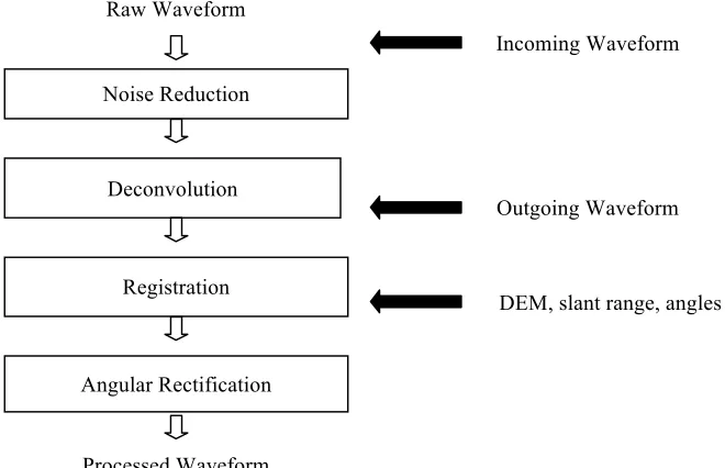
In this chapter, we first describe the datasets used for testing the proposed processing chain, namely real waveform Carnegie Airborne Observatory (CAO) data and simulated waveform via the Digital Imaging and Remote Sensing Image Generation (DIRSIG) model. Next, the processing chain is presented in a stepwise fashion that follows the diagram in Figure 2.1. This approach assumes that the following information is available for each of the per-pixel waveform LiDAR signals: (i) outgoing waveform, (ii) incoming waveform, (iii) angular information, including zenith and azimuth, (iv) slant range, and (v) a digital elevation model (DEM) for the site of interest. Finally, metrics for evaluating the performance of the processing chain are introduced for both simulated and real waveform data in order to provide a comprehensive validation of the approach. We recognize that the proposed framework and methodology may not be optimal for all waveform LiDAR users, depending on their specific applications or computational resource limitations. However, the purpose of this study was to develop, validate, and propose a standardized waveform preprocessing approach for waveform LiDAR researchers and engineers to extract more representative and accurate 3D structural parameters from remotely sensed scenes. Outputs from this chapter have been published as follows:

• Wu J., J.A.N. van Aardt, and G.P. Asner. A Comparison of Signal Deconvolution

Algorithms Based on Small-Footprint LiDAR Waveform Simulation. IEEE Transactions on Geoscience and Remote Sensing 49(6): 2402-2414, 2011 [42].

• Wu J., J.A.N. van Aardt, J. McGlinchy, and G.P. Asner. A Robust Signal

(39)

[image:39.612.130.460.81.294.2]

Figure 2.1. A flowchart of the waveform LiDAR preprocessing chain

2.1

Methods

2.1.1

Available data

2.1.1.1

Real waveform and associated field data

The study area for this research effort is comprised of a section of land within and surrounding Kruger National Park (KNP) in South Africa (Figure 2.2). The area is bounded by (22°8’00” S; 30° 34’52”E) and (25° 32’ 48”S; 32° 2’ 50” E) and spans a west-east land use gradient. This gradient is defined by sampling in Bushbuckridge (communal rangelands; high rural population density), Sabie Sands game reserve (private conservation area), and Kruger National Park (state-owned conservation area). The topography is gently undulating with a slowly decreasing terrain height toward the east, with an average altitude of approximately 450m above mean sea level. Vegetation communities are influenced largely by geomorphological and pedological processes at

Processed Waveform Noise Reduction

Raw Waveform

Registration

Angular Rectification Deconvolution

Incoming Waveform

Outgoing Waveform

(40)

the landscape level. Dominant geology includes granite and gneiss with local intrusions of gabbro. Vegetation has a discontinuous overstory of woody plants, mostly in the 2-5m height category, and a herbaceous layer dominated by C4 grasses [44]. The vegetation communities are classified as granite lowveld or gabbro grassy bushveld according to Muncina et al. [45]. Therefore, the waveform and field data we collected have enough physical variability in terms of the wide range of woody structure and biomass level for further analysis.

Figure 2.2. The study area and associated land use gradient in South Africa

Waveform LiDAR data were collected by the Carnegie Airborne Observatory (CAO) alpha system, using a custom-built Optech ALTM 3100EA system (Figure 2.3) with an outgoing pulse width of 16ns, a laser wavelength of 1064nm, a footprint of 0.56m, and a temporal resolution of 1ns, which corresponds to 0.15m vertically.

(41)

[image:41.612.184.430.152.473.2]

crown height and diameter at breast height (DBH) to be used as input to allometry equations for calculation of woody biomass. Herbaceous biomass was directly measured by the weight of dry grass within a 0.5×0.5m grid at each plot center.

Figure 2.3. CAO Alpha system with the ALTM 3100 waveform LiDAR system.

[image:41.612.217.389.540.674.2]

(42)

2.1.1.2 Simulated LiDAR waveform data

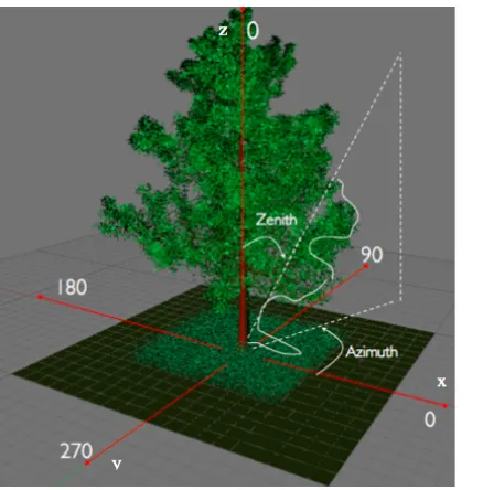
Virtual scenes that combined a 3D deciduous tree, above-ground grass layer, and ground were created as the input for the DIRSIG simulation (see appendix A.1 for more details) by using the tree generation software “Arbaro” [46] and rendered using the open source 3D graphics application “Blender” [47] (Figure 2.5). Materials including leaves, branches, grass, and ground with valid emissivity and extinction coefficients, as measured from actual vegetation, were mapped to each facet of these 3D models. This enabled us to comprehensively simulate the process of laser pulse interaction with vegetation, including absorption, reflection, and transmission at each facet. We created a 3D real world coordinate system (x,y,z) with the center of the tree base as origin, in order to better characterize the relative position between the scene and the laser pulse. The zenith and azimuth angles were used, as Figure 2.5 shows, to define the trajectory of each laser pulse.

[image:42.612.125.344.383.605.2]

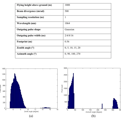
The LiDAR system configuration is another important input required for accurate waveform simulation. The parameters that were used for configuring the LiDAR system are summarized in Table 2.1. The goal was to match our virtual system with

Figure 2.5. An example of a virtual scene for generating simulated waveform LiDAR:

• Ground: 20m×20m (x, y)

• Grass: 12m×12m×1m (x, y, z)

(43)

flying height (1000m) and beam divergence (500 mrad) were used to generate the size of small-footprint waveform simulations (0.5m). The selection of pulse width was motivated by the outgoing pulse width of 16ns, as implemented in the operational waveform LiDAR data collected by the CAO using a custom-built Optech ALTM 3100EA system; the same applies to the selection of 1ns as sampling resolution (time bin) and 1064nm as wavelength. This allowed for the simulation results to be directly compared to operational or real data. We also added 2ns, 4ns, and 8ns outgoing pulse widths for simulation purposes. This was due to the facts that the 2ns outgoing pulse width (near perfect system impulse response) can be used to generate the approximated or truth dataset and the 4ns/8ns pulse widths are the standard settings for CAO wLiDAR and other commercial systems. These pulse widths therefore can be used as intermediate widths between 2ns and 16ns to test the robustness of the processing chain at different outgoing pulse widths.

We furthermore restricted the outgoing pulse shape to approximate a Gaussian distribution, based on our observation of the actual outgoing pulses from the CAO: the shape of the actual pulses closely approximates a “Gaussian” distribution and the observed asymmetry is minimal. It was also observed that the shape of the actual outgoing pulses varies in terms of the slope and intensity. We therefore used a Gaussian approximation in order to maintain consistency in the shape of the outgoing pulse across all the waveforms for our simulation.

(44)

the approximated or truth dataset in order to facilitate comparisons with the angular, rectified, off-angle waveforms.

Figure 2.6. Histogram of the zenith (a) and azimuth (b) angle distributions based on real waveform LiDAR data collected by CAO

2.1.2 Noise reduction

The raw incoming waveform typically exhibits a certain noise level due to sensor

Flying height above ground (m) 1000

Beam divergence (mrad) 500

Sampling resolution (ns) 1

Wavelength (nm) 1064

Outgoing pulse shape Gaussian

Outgoing pulse width (ns) 2/4/8/16

Footprint (m) 0.56

Zenith angle (°) 0, 5, 10, 15, 20

[image:44.612.82.502.152.569.2]

Azimuth angle (°) 0, 90, 180, 270

TABLE 2.1

A DESCRIPTION OF THE LIDAR SYSTEM CONFIGURATION

(45)

noise was simulated using uniformly distributed pseudo-random numbers, assuming white noise, and was added to each waveform in order to approximate the real LiDAR signal-to-noise ratio, which is unknown. This approach also served to test the robustness of processing steps, e.g., deconvolution algorithms, against noise. The amplitude of the noise (Figure 2.7) was estimated by averaging the absolute difference between the noisy and the smoothed waveform data collected by Carnegie Airborne Observatory systems. The resultant waveforms arguably may not reflect the exact noise level and distribution in real waveform LiDAR systems, while the actual signal-to-noise ratio may also vary between different system types and configurations. However, considering that this effort (i) represented a relative comparison of different deconvolution approaches, (ii) used the same waveform data with the same added noise, and (iii) that the high frequency noise is dominated by low frequency signals in such systems, we believe that the impact induced by the relatively simplistic noise estimation was minor.

(46)

derivative analysis (e.g., zero crossing point) or integration of the area over the frequency spectrum (e.g., 99% of the underlying area). However, the complexity of automated approaches for real datasets and the ability of deconvolution to overcome certain noise level might negate the need for additional complexity.

Figure 2.7. Illustration of the waveform noise filtering: (a) Real (raw) waveform data collected by the Carnegie Airborne Observatory system and (b) the smoothed waveform

following frequency-based noise filtering. Note: a negative noise level shift of 11 units was applied to the raw signal first to avoid the potential frequency leakage caused by the

sharp edge at the inflection point (signal on/off)

Figure 2.8. A typical frequency representation of a waveform signal. A cut-off frequency threshold of 0.2GHz was selected based on visual assessment of filtering results; any

frequency component above 0.2GHz was attributed to noise and set to zero.

Threshold

(47)

2.1.3

Deconvolution

The raw incoming waveform is usually smeared and the effective temporal or vertical resolution decreases due to the non-perfect outgoing pulse signal (e.g., distorted Gaussian, instead of delta function) and the receiver impulse response. Theoretically, such a loss of resolution can be recovered by deconvolving the system response from the measured signal. We therefore introduce a quantitative comparison approach between the three most widely used deconvolution techniques in the waveform LiDAR processing literature, namely the Richardson-Lucy (RL), Wiener filter (WF), and non-negative least squares (NNLS) algorithms.

In order to evaluate the impact of and need for deconvolution on waveform processing, especially for vegetation applications, we tested the algorithms in the context of two vegetation structural assessments: (i) ability to recover the true cross-section profile of an illuminated object, based on the waveform simulation of a virtual 3D tree model (Figure 2.5) and (ii) the ability to differentiate variation in herbaceous biomass, based on the waveform simulation of virtual grass patches.

2.1.3.1

Recovering the true cross-section of vegetation

(48)

Observatory [46]. This was followed by the application of the three deconvolution algorithms to the simulated return signals and a comparison of the resultant deconvolved signals with the true cross-section data (approximated by the 2ns outgoing pulse). Two waveform datasets, namely the 2ns true response and the deconvolved comparison, should be similar in terms of shape if the deconvolution functioned properly. We simulated the complexity and diversity of natural trees by generating six different virtual 3D trees at a fine- or object-scale, whose specifications and rendered images are listed and shown in Table 2.2 and Figure 2.9, respectively. Each tree plot consisted of branches, leaves, and ground associated with their respective valid emissivity and extinction coefficients [43]. The plot for each tree was divided into a 40x40 pixel grid with a waveform footprint size equal to 0.5m. This resulted in a waveform with 225 time bins, from 24.995m to -8.605m “above ground”, at an increment of 0.15m for each pixel after implementing the simulation. Finally, three sets of simulated waveforms were generated for each tree plot for outgoing pulse widths of 2ns, 8ns, and 16ns to check the monotonic trend of the deconvolution comparison results in terms of outgoing pulse width. A 4ns simulation was added for preprocessing validation based on feedback from journal reviewers to ensure that the preprocessing chain can be applicable to different operational sensors specifications.

Three metrics were used to assess the performance of the respective deconvolution algorithms in terms of recovering the cross-section:

1. Root mean square error (RMSE) value between the truth and the deconvolved waveform:

(14)

where is the truth cross-section approximated by the direct simulation results

using an outgoing pulse width equal to 2ns. corresponds to the deconvolved

waveform using an outgoing pulse widths equal to w =8, and 16ns. m and n are the number of time bins for each waveform and the total number of waveforms for the plot (e.g., m=225, n=1600 in this paper), respectively.

RMSE=



P_δ,2(t)−Pδ,w(t)

(

)

2

m

∑

n

∑

m×n

€

˜ P _δ,2(t)

€

(49)

2. We also evaluated the waveform sensitivity to local peak detections by determining where the sign of the first derivative of the waveform changes for different deconvolution approaches. This is defined as:

(15)

True detection is defined by the time bin index of a detected local peak from the deconvolved waveforms that agrees with a true peak, which is extracted from the 2ns waveform simulation for each of the six trees.

3. Finally, another important metric, called the f