Scanning acoustic microscopy for GDL water distribution characterization

(1)

Rochester Institute of Technology

RIT Scholar Works

Theses Thesis/Dissertation Collections

2010

Scanning acoustic microscopy for GDL water

distribution characterization

Christopher McDade

Follow this and additional works at:http://scholarworks.rit.edu/theses

This Thesis is brought to you for free and open access by the Thesis/Dissertation Collections at RIT Scholar Works. It has been accepted for inclusion in Theses by an authorized administrator of RIT Scholar Works. For more information, please [email protected].

Recommended Citation

(2)

SCANNING ACOUSTIC MICROSCOPY

FOR GDL WATER DISTRIBUTION

CHARACTERIZATION

by

C. Lee McDade

A Thesis Submitted in Partial Fulfillment of the Requirements for the degree of

Master of Science in Mechanical Engineering

Approved By:

Dr. Satish G. Kandlikar _______________________________

Professor of Mechanical Engineering (Thesis Advisor)

Dr. Navalgund Rao _______________________________

Associate Professor of Imaging Science

Dr. Maria Helguera _______________________________

Assistant Professor of Imaging Science

Dr. Tuhin Das _______________________________

Assistant Professor of Mechanical Engineering

Dr. Edward C. Hensel / Dr. Alan H. Nye _______________________________ Department Head of Mechanical Engineering (Department Representative)

Rochester Institute of Technology

(3)

Permission to Reproduce

Title:

Scanning Acoustic Microscopy for GDL Water Distribution

Characterization

I, Christopher Lee McDade, hereby grant permission to the Wallace Memorial Library of

Rochester Institute of Technology to reproduce my thesis in the whole part. Any

reproduction will not be for commercial use or profit.

(4)

i

Abstract

The objective of this research was to identify and apply possible acoustic imaging

techniques for water transport studies in PEM fuel cell diffusion mediums. To accomplish

this, a scanning acoustic microscope (SAM) was designed and built along with dedicated

control and analysis software to implement all investigative tests and scans. The results of the

study were in two parts, acoustic response characterization of the fibrous material and

implementation of the developed imaging technique for water saturation distribution

characterization.

Having used a focused 30 centered wide band transducer with focal point FWHM beam diameter of 90 the target material ensured a number approximately equal to one given the average fiber diameter around 8. The result was a diffractive acoustic response subject to phase sensitive interference. Traditional ultrasonic techniques

for material characterization or imaging were inapplicable so a signal correlation ratio

method was developed which relies on the variations in acoustic responses between two

scans. Results from different GDL samples at varying levels of saturation were compared to

(5)

ii

List of Figures

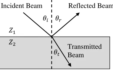
Figure 1.3-1: Specular beam reflection rays. ... 5

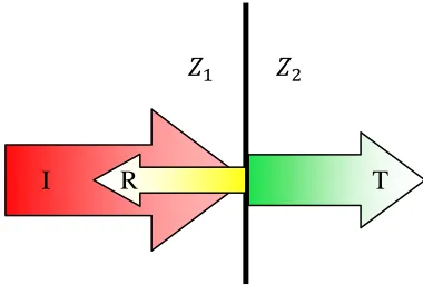
Figure 1.3-2: Impedance boundary pulse energy division... 6

Figure 1.3-3: Diffractive scattering polar plots. [5] ... 7

Figure 1.4-1: Beam intensity profile as a function of aperture distance. ... 10

Figure 1.5-1: B-scan image of 12.7µm diameter tungsten wire at transducer focal depth... 13

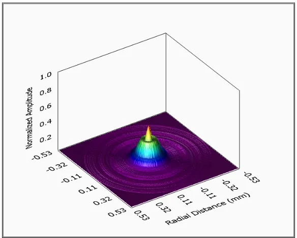
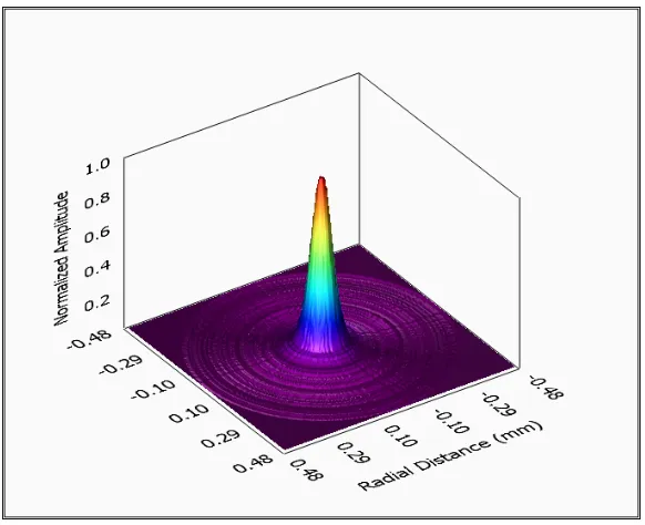
Figure 1.6-1: Beam profile plot illustrating full width half maximum. ... 14

Figure 1.6-2: Beam intensity profile map for an unfocused rectangular aperture. ... 15

Figure 1.7-1: Example A-line envelope. [10] ... 18

Figure 1.8-1: Typical transducer construction. ... 18

Figure 1.8-2: Piezoelectric cartoon. ... 19

Figure 1.8-3: KLM Transducer electrical equivalency model. ... 21

Figure 1.8-4: Transducer electrical model ... 22

Figure 1.9-1: M-scan orientation. ... 25

Figure 1.9-2: B-scan orientation. ... 25

Figure 1.9-3: C-scan orientation. ... 26

Figure 3.1-1: Optical image of Toray-120 GDL with 20% PTFE loading (2x2mm). ... 77

Figure 3.2-1: Optical image of Toray-120 GDL with 90 micron diameter dot (0.8x0.8mm)... 81

Figure 3.2-2: Plot illustrating random nature of received echo signals. ... 82

Figure 3.2-3: Plot of detected peaks with exponential fit trend line and one standard deviation boundaries. ... 83

Figure 3.2-4: Plot illustrating the decrease in acoustic attenuation with increasing saturation. ... 84

Figure 3.2-5: Typical C-scan images illustrating change after differential pressure application. (a) C-Scan_263 Dry Reference Image, (b) C-Scan_268 image from 0.5psi ∆p. ... 86

Figure 3.2-6: Two method for identifying regions of water intrusion. Sample is of Toray 120 plain after 0.07psi ∆p . (a) C-Scan_128-131 image difference, (b) C-Scan_128-131 scan correlation. ... 87

Figure 4.1-1: System diagram showing connectivity. ... 89

(8)

v

Figure 4.1-3: S.A.M. Part Label. ... 94

Figure 4.1-4: Cross-sectional image of microscope base. ... 95

Figure 4.1-5: Sample Brackets. Bottom (Left) and Top (Right). ... 96

Figure 4.3-1: Example M-scan Brightness Plot. ... 102

Figure 4.3-2: Encoder phases A and B offset by 90°. ... 104

Figure 5.1-1: Pulse Reference Setup. ... 107

Figure 5.1-2: Received pulse from steel plate reflection. ... 107

Figure 5.1-3: Pulse frequency response from steel plate reflection. ... 108

Figure 5.1-4: Beam profile scan setup. ... 109

Figure 5.1-5: Near field half amplitude beam profile. ... 110

Figure 5.1-6: Peak Amplitude beam profile. ... 111

Figure 5.1-7: Far field half amplitude beam profile. ... 111

Figure 5.1-8: Beam Intensity Map. ... 112

Figure 5.1-9: Beam profiles at the focal depth for filtered and un-filtered A-line data. The applied filter used a hamming window with a low cutoff frequency of 20MHz. ... 113

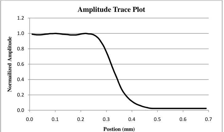
Figure 5.1-10: Trace of echo amplitude scanned over sharp edge. ... 114

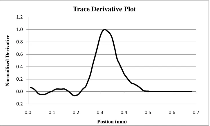
Figure 5.1-11: Derivative plot of echo amplitude trace. ... 115

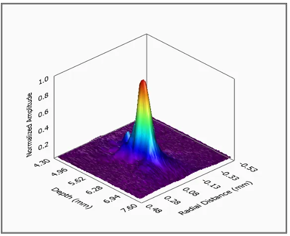
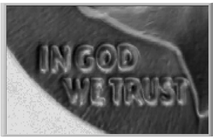
Figure 5.1-12: Reconstructed dime surface. ... 116

Figure 5.1-13: Backscatter plot of dime scan. ... 116

Figure 5.2-1: A-line samples from Toray -120 Plain. GDL C-scan_144. ... 118

Figure 5.2-2: A-line samples from Toray -120 Plain. GDL C-scan_144. ... 118

Figure 5.2-3: Optical image of Toray-120 GDL with 90 micron diameter dot (0.8x0.8mm)... 119

Figure 5.2-4: B-scan of Toray-120. GDL-B-scan_16. ... 120

Figure 5.2-5: Video image results for frame 1 of Toray-060 with 20% PTFE. GDL-B-scan_48. ... 122

Figure 5.2-6: Video image results for frame 30 of Toray-060 with 20% PTFE. GDL-B-scan_48. ... 122

Figure 5.2-7: C-scan images depicting A-line backscatter over time-gate 7.87-8.07µs arrival time. C-scan-285 ∆p=0.07psi. ... 124

Figure 5.2-8: C-scan images depicting A-line backscatter over time-gate 7.87-8.07µs arrival time. C-scan-292 ∆p=2psi (Bottom). ... 124

(9)

vi

Figure 5.2-10: C-scan images depicting A-line backscatter over time-gate 8.17-8.37µs

arrival time. C-scan-292 ∆p=2psi. ... 125 Figure 5.2-11: B-line backscatter trends for both the dry (0.07psi ∆p, C-scans-285) and

the wet (2psi ∆p, C-scan-292) scans. ... 127 Figure 5.2-12: Echo amplitude trend for both the dry (0.07psi ∆p, C-scans-285) and the

wet (2psi ∆p, C-scan-292) scans. ... 129 Figure 5.2-13: Individual echo amplitude fit exponential decay trends with one

standard deviation bounds and 10% echo points plotted. Dry (0.07psi

∆p, C-scans-285) case. ... 129 Figure 5.2-14: Individual echo amplitude fit exponential decay trends with one

standard deviation bounds and 10% echo points plotted. Wet (2psi ∆p,

C-scan-292) case. ... 130

Figure 5.2-15: ImageJ volume rendering of C-scan-34 Toray-120 plain dry reference,

∆p=0.07psi. ... 132 Figure 5.2-16: ImageJ volume rendering of C-scan-34 Toray-120 plain dry reference,

∆p=0.07psi C-scan-36 Toray-120 plain wet, ∆p=1.0psi). ... 132 Figure 5.2-17: C-scan images of Toray-060 after 0.07psi ∆p depicting A-line

backscatter over 0.10µs time-gate. C-scan-30 with time-gate

7.95-8.05µs and pulser gain of 0dB. ... 134 Figure 5.2-18: C-scan images of Toray-060 after 0.07psi ∆p depicting A-line

backscatter over 0.10µs time-gate. C-scan-31 with time-gate

8.15-8.25µs and pulser gain of 20dB. ... 134 Figure 5.2-19: C-scan images of Toray-060 after 2psi ∆p depicting A-line backscatter

over 0.10µs time-gate. C-scan-32 with time-gate 7.95-8.05µs and pulser

gain of 0dB... 135

Figure 5.2-20: C-scan images of Toray-060 after 2psi ∆p depicting A-line backscatter over 0.10µs time-gate. C-scan-33 with time-gate 8.15-8.25µs and pulser

gain of 20dB... 135

Figure 5.2-21: A-line of Toray-030 GDL with a 20dB amplified region. ... 137

Figure 5.2-22: Propagation speed scan setup. ... 138

Figure 5.2-23: A-line of Toray-120 GDL with a 0.005” gap between support plate.

C-scan-60. ... 139

Figure 5.2-24: Identified echoes from C-scan-60 plotted. ... 140

Figure 5.2-25: Histogram of calculated speed of sound through GDL sample. ... 141

Figure 5.2-26: Deviation in time-of-flight between known water path duration and

measured plotted over scanned area. ... 141

(10)

vii

Figure 5.3-1: Example dry and wet A-lines after 0.5psi differential pressure

application. Resulting correlation ration of 0.76. C-scans 296-300. ... 146

Figure 5.3-2: Example dry and wet A-lines after 0.5psi differential pressure application. Resulting correlation ration of 68.09. C-scans 296-300. ... 146

Figure 5.3-3: C-scan-317 dry reference scans backscatter, 0.07psi ∆p. ... 147

Figure 5.3-4: C-scan-317 dry reference scans backscatter, C-scan-321 saturated scans backscatter, 0.5psi ∆p. ... 147

Figure 5.3-5: Relative amplitude image difference between C-scan-317 & 321, 0.5psi ∆p. ... 149

Figure 5.3-6: Relative amplitude correlation ratio between C-scan-317 & 321, 0.5psi ∆p. ... 149

Figure 5.3-7: Relative amplitude image difference between C-scan-128 & 131, 0.07psi ∆p. ... 150

Figure 5.3-8: Correlation ratio between C-scan-128 & 131, 0.07psi ∆p. ... 150

Figure 5.3-9: A-line comparison location 1 for C-scan-128 & 131. ... 151

Figure 5.3-10: A-line comparison location 2 for C-scan-128 & 131. ... 152

Figure 5.3-11: Silicon covered pin hole scan orientations. ... 153

Figure 5.3-12: Dry scans backscatter over time-gate 8.4-8.65µs. 0.07psi ∆p C-scan-108 orientation 1. ... 154

Figure 5.3-13: Wet scans backscatter over time-gate 8.4-8.65µs. 1.0psi ∆p C-scan-110 orientation 1. ... 154

Figure 5.3-14: Correlation ratio between C-scan-108 & 110, orientation 1. ... 155

Figure 5.3-15: Dry scans backscatter over time-gate 8.0-8.4µs. 0.07psi ∆p. C-scan-116 orientation 2. ... 156

Figure 5.3-16: Wet scans backscatter over time-gate 8.0-8.4µs. 1.0psi ∆p.C-scan 122 orientation 2. ... 156

Figure 5.3-17: Correlation ratio between C-scan-116 & 122, orientation 2. ... 157

Figure 5.3-18: Fractional coverage as a function of ∆p for Toray PTFE comparison series. ... 160

Figure 5.3-19: Total cells identified as a function of ∆p for Toray PTFE comparison series. ... 160

Figure 5.3-20: Average cell size as a function of ∆p for Toray PTFE comparison series. ... 161

Figure 5.3-21: Average normalized B-line backscatter Toray-120 20% PTFE Loading. C-scan-229 series. ... 162

Figure 5.3-22: C-scan backscatter with B-line std. dev. bars as a function of ∆p for Toray PTFE series. ... 163

(11)

viii

Figure 5.3-24: Average total cells identified for Toray-120 20% PTFE loading. ... 164

Figure 5.3-25: Average cell size for Toray-120 20% PTFE loading. ... 165

Figure 5.3-26: 2x2mm optical image of Toray-090, MPL side. ... 166

Figure 5.3-27: 2x2mm optical image of Toray-090, non-MPL side. ... 167

Figure 5.3-28: 2x2mm optical image of carbon cloth A with 10% PTFE. ... 167

Figure 5.3-29: Correlation ratio image results for Toray-090 sample with MPL facing up after 0.15psi saturation pull. C-scan-359 series. ... 169

Figure 5.3-33: Correlation ratio image results for Toray-090 sample with MPL facing down after 0.15psi saturation pull. C-scan-369 series. ... 171

Figure 5.3-37: Correlation ratio image results for Toray-120 sample with 20% PTFE loading after 0.15psi saturation pull. C-scan-307 series. ... 173

Figure 5.3-41: Correlation ratio image results for carbon cloth sample after 0.15psi saturation pull. C-scan-274 series. ... 175

(12)

ix

Figure 5.3-45: Fractional coverage as a function of ∆p for Toray type comparison

series. ... 178

Figure 5.3-46: Total cells identified as a function of ∆p for Toray type comparison

series. ... 178

Figure 5.3-47: Average cell size as a function of ∆p for Toray type comparison series. ... 179 Figure 5.3-48: Average normalized B-line backscatter Toray-090 with MPL facing up.

C-scan-350 series. ... 180

Figure 5.3-49: C-scan backscatter with B-line std. dev. bars as a function of ∆p for

Toray type comparison series. ... 180

Figure A.1-1: Observed A-line noise standard deviation as a function of

pulser/receiver gain. (Log base ten gain scale) ... 189

Figure A.1-2: Observed A-line noise standard deviation as a function of

pulser/receiver gain. (Linear gain scale) ... 189

Figure A.2-1: Water column data points with 95% confidence interval. ... 193

Figure A.2-2: Pressure sensor calibration data points with corresponding linear fit

lines. ... 198

Figure A.3-1: Two A-line examples used to illustrate the backscatter attributes. ... 202

Figure A.4-1: Amplitude trace plot of scanned sharp edge with theoretical ideal trace. ... 205

Figure A.4-2: Derivative plot of amplitude trace with identified interpolation points for FWHM calculation. ... 206

(13)

x

List of Tables

Table 3.2-1: Listing of applied differential pressures used for the corresponding scans

with their respective exponential decay fit constants. ... 84

Table 5.1-1: Tabulated results of beam profile characterization. ... 112

Table 5.2-1: Tabular description for example C-scan images. ... 126

Table 5.2-2: Tabular results for B-line backscatter plots from example C-scan saturation study. ... 127

Table 5.2-3: Tabular results for echo amplitude trends from example C-scan saturation study. ... 130

Table 5.3-1: Pressure application series for all saturation distribution tests. ... 159

Table A.2-1: Pressure column variable values. ... 192

Table A.2-2: Pressure estimates with 95% confidence interval. ... 193

Table A.2-3: Pressure sensor 1 calibration data points with pressure errors. ... 196

Table A.2-4: Pressure sensor 1 calibration data linear fit results. ... 196

Table A.2-5: Pressure sensor 2 calibration data points with pressure errors. ... 197

Table A.2-6: Pressure sensor 2 calibration data linear fit results. ... 197

Table A.3-1: A-line backscatter and estimated error values as propagated from A-line voltages. ... 202

Table A.4-1: Beam profile amplitude trace values of interest for FWHM calculation. ... 205

(14)

1

Introduction

Fuel cells show promise in the future of alternative energy sources. Among the most

capable is the Proton Exchange Membrane (PEM) fuel cell. PEMFCs are currently being

developed for transportation, portable and stationary power sources given their relatively

high energy conversion efficiency, zero emissions, and low operating temperatures and

pressures. Even with their relative success, issues still need to be resolved. One of the

primary areas of research is water management and its effect on the overall cell performance

and durability.

A key component to water management and control is the gas diffusion layer (GDL),

commonly constructed of carbon paper. Its role within the cell is to ensure even distribution

of reactant gasses and removal of excess product water while not inhibiting the flow of

electrons between cells. Two common problems of poor water management are flooding and

membrane dehydration. Excess water can inhibit reactant gas transport while improper

membrane hydration reduces proton conductivity. To solve these problems, knowledge of the

propagation characteristics of gas and water within the GDL is required. With varying levels

of success, neutron and x-ray imaging techniques have been used to study water distribution

within the GDL. While both methods can resolve high resolution 2D maps of water in-plane,

neither can produce three dimensional distributions. In an effort to overcome this deficiency

ultrasonic imaging was proposed.

Ultrasound imaging is a well established technology that has many applications for

three dimensional reconstruction. The most common use is for medical applications, where

ultrasound has been successfully utilized to image most parts of the human anatomy. Equally

successful is the use of ultrasound to scan for internal fractures or anomalies within

performance critical parts. However the use of ultrasound to image a GDL, a highly

inhomogeneous material with micron size features, presents a new challenge. With the use of

high frequency transducers and tuned signal processing, this objective is being pursued.

Ultimately, extracting meaningful information and new insights to the water distribution

(15)

2

Chapter 1: Ultrasound Theory

1.1-Applying Ultrasound

Ultrasound is defined as sound waves having frequencies higher than 20 , the typical upper limit for human hearing. It is used for a variety of purposes, medical imaging,

flaw detection, short range distance measurements, acoustic cleaning, etcetera. Operating

frequencies can range from 100 to 100 depending on the application [1].

Unlike light, ultrasound waves need an elastic medium to propagate, relying on the

particles connective forces to translate the wave. These waves are subject to typical

macroscopic effects of all waves, namely reflection, refraction, and diffraction [1].

When applying ultrasound to a target sample a short pulse of some primary frequency

is introduced to the object via an ultrasound transducer. This pulse then travels through the

material at approximately constant speed. When an echo generating object or scatterer is

encountered by the high frequency pulse some of its energy is reflected back to the

transducer. This echo pulse is then converted into a time varying voltage, typically called the

A-line signal, which is then analyzed [2]. While the time of travel is converted into scatterer

depth, relative echo signal amplitude and phase can be used in material property

characterization [3].

The process of pulse/echo imaging can be approximated as a linear system. It is

common to model the series of events as a series of time convolved modifiers or effectively a

frequency domain series of filters.

, , , ,

, ,

(1.1-1)

, , ! " !, , #$2% " ~'(_{" #$)4+}

(16)

3

These functions include the transducers effect, a_-t, on the pulse as well as the functions that describe the attenuation, a_/t, diffraction, a₀r₂, z, t, and scattering physics, a₄t. Note the use of two transducer, diffraction and attenuation functions to account for the two

way travel of the pulse and both transmit and receive events.

1.2-Wave Propagation

The governing equation for wave motion and propagation is given in equation 1.2-1,

567

5$₇ 8 9 5 !_:;<

5!! (1.2-1)

Where and 9 are the body forces and material density respectively. The connection

between stress and strain are listed in equation 1.2-2 assuming a linear relation where = and are the first and second Lame’s constants.

67 2?78 =7?7 (1.2-2)

= 8 @@. :;< 8 @!_{:;< 9} 5!:;<

5!! (1.2-3)

Time harmonic solutions to these equations come in the form where w is the angular velocity

of the wave and is the wave number.

: :B#$C)D E (1.2-4)

The two are related by the material property phase velocity which is not only

dependent on the material properties but also the type of wave motion, distortional or

dilatational.

(17)

4

For distortional waves where shear and rotation of particles define their motion, the

propagation speed is defined by equation 1.2-6 below.

FH I₉ (1.2-6)

For dilatational waves, dominant form in liquids, where the particle motion is in-line with the

wave propagation the phase velocity becomes,

FJ I= 8 2₉ (1.2-7)

or in engineering constants where K is the Young’s modulus and L is the Poisson’s ratio of the material.

FJ I_{91 2LL 8 1}K1 L (1.2-8)

For fluids where the Poisson’s ratio approaches one half, zero viscosity, the propagation

speed is then expressed in terms of the fluids bulk modulus.

FJ IM₉ (1.2-9)

There are many vibratory modes in which ultrasound can propagate but longitudinal

waves are the most common in imaging applications [1]. This can be attributed to liquids

inability to support shear waves and the relatively straight forward implementation of

(18)

5

1.3- Backscatter Effects and Attenuation

The ability of an object to produce an echo signal is dependent on its

reflection/scattering characteristics. In order for ultrasound waves to be reflected or scattered

there needs to be an interface at which there is a change in acoustic impedance, Z [1]. N is a material property which quantifies the resistance of its particles motion induced by a sound

wave [4]. Acoustic impedance is defined by the following formula where 9_{is the material} density and F is the propagation speed for the material.

N 9F (1.3-1)

For example, water has an average propagation speed of 1,481OPQ and an acoustic impedance of 1.48$10R S/!O at standard temperature and pressure [1]. If a propagating

wave encounters a material with a different acoustic impedance than the coupling medium

[image:18.612.214.405.420.542.2]

vibratory energy will be scattered in a manner dependent on the materials size and shape [2].

Figure 1.3-1: Specular beam reflection rays.

There are three general categories in which a scattering boundary can fall, specular,

diffractive, and diffusive. The first being a scatterer with a length scale much larger than the

sound wavelength. In this case the pulse wave reflection and refraction will be specular,

allowing the waves to be approximated as rays following Snells’s law for reflection and

refraction.

Reflected Beam Incident Beam

Transmitted Beam

UH

U U NQ

(19)

6

O)VU O)VU

F_Q

F! (1.3-2)

The strength of the reflected and transmitted waves can be approximated by the

relation between the materials acoustic impedances [2].

WX N_N!FYOUNQFYOU

!FYOU8NQFYOU (1.3-3)

ZX _N 2N!FYOU

!FYOU8NQFYOU (1.3-4)

[image:19.612.218.408.358.490.2]

Where U_andU are the incident and transmitted ray angles respectively. The echo signal strength for this category of reflector is relatively strong and independent of frequency [1].

Figure 1.3-2: Impedance boundary pulse energy division.

The second and most complicated category, diffractive, is for objects with sizes

comparable to the ultrasound wavelength. Generally the echo signal strength from this

category of scatterer is 10 Y 30'[ lower than that of specular boundaries and are dependent on the pulse frequency [1]. For this size scale the scattering pattern is generally modeled by

taking the scatterer surface as the source of the reflected waves. The result of diffractive

interference from all infinitesimal point sources on the surface construct the scattering

pattern. Modeling the backscatter for this regime is difficult and exact solutions for only

some simple geometries have been solved analytically [5].

N! NQ

(20)

7

Figure 1.3-3: Diffractive scattering polar plots. [5]

In this scattering regime, where the number is approximately equal to one, a relative small

change in the relation between the wavenumber, , to the scatterer size, , can result in a large change in the scattering pattern. This effect makes ultrasonic signals difficult to

interpret and is illustrated in figure 1.3-3.

2+₌ (1.3-5)

An additional phenomenon that is relevant for this scatterer size regime is speckle.

Given that the feature sizes of the reflectors are on the order of the pulse wavelength multiple

scatterers can be present in the transducers resolution cell. Constructive and destructive

(21)

8

transducer. This produces a texture in the resulting image known as speckle. Statistical

analysis of the speckle pattern can be used to extract useful tissue characteristics and can

enhance image contrast [2].

The third category is for scatterers that have dimensions much smaller than the

ultrasound wavelength, \ 1. Scatterers possessing this size scale produce very weak reflections but whose amplitude is highly dependent on the pulse frequency, ]~^ [1]. It is also noted that individual echoes from surface roughness features of this size regime exhibit

insignificant interference with each other. This given the small phase difference between

reflections from high and low points of the surface [5].

Derived from an exact solution, Lord Rayleigh developed an expression for the

radiating intensity from an elastic sphere much smaller than the irradiating ultrasound

wavelength.

] ]

^R 9! _

3C1 9! ₉ Q G EFYO` 1 8 2 9! ₉

Q

G 8 a1

bc

bdef

!

(1.3-6)

Subscript 2 in equation 1.3-6 indicates the spheres density, 9_!, and compressibility , _! [5]. Note the scattered intensities fourth power dependence on frequency and the sixth power

dependence on the scatter radius.

A major obstacle to overcome in any ultrasound imaging system when depth

penetration and resolution is of concern is attenuation. During a wave’s propagation its

amplitude drops with distance exponentially [2]. Reduction in the wave’s energy or intensity

can be attributed to absorption and scattering losses. The combined effect of these two losses

defines attenuation and is approximately linearly dependant on frequency for most tissues.

This loss is accounted for with the material transfer function (MTF) in the frequency domain

and the material impulse response function (mirf) in the time domain for modeling purposes.

The resulting pulse, , , after a given distance traveled is calculated by convolving the initial pulse with the mirf.

(22)

9

This is equivalent to multiplying the Fourier transformed pulse with the MTF [6] where % is the attenuation factor and β_h is an excess dispersion term to account for causality [7].

ZX, #$i (1.3-8)

i % )j B 8 klm (1.3-9)

% %B8 %Q||o (1.3-10)

The effect is an exponential decay in the pulse amplitude with distance. Generally,

lossy materials act as a lowpass filter, causing a shift towards zero in the center frequency.

pqr s %_2tQ (1.3-11)

This model also accounts for phase velocities dependence on frequency, known as

dispersion, this effect is where propagation speed increases with frequency.

Fu FB FB !_k_l

u (1.3-12)

When the non-linear response of a medium is taken into account the phase velocity then

depends on the displacement gradient 5: 5⁄ where :, is the particle displacement [1].

5:!

5! FB

!

a1 8 5:_5ew x⁄ y! 5:!

5! (1.3-13)

Where [ ⁄ is the non-linear parameter of the material. The consequence is that the higher pressure or higher frequency regions of the wave will travel faster than the lower pressure

(23)

10

1.4-Sound Field

The sound field of a transducer can be divided into two regions, the near field and the

far field, or the Fresnel and Fraunhofer regions respectively. The near field is defined as the

beam section in front of the transducer element where the sound field undergoes a series of

maxima and minima, ending with the last maxima [1].

Figure 1.4-1: Beam intensity profile as a function of aperture distance.

The region after this last maximum in known as the far field where the waveform

intensity gradually decays. The size and shape of the near field, z, is governed by diffraction but its length can be approximated with knowledge of the transducer frequency, element

diameter, and material sound velocity [8].

z {_4F! {₄₌! (1.4-1)

Due to the near fields variation in waveform intensity it is difficult to perform any amplitude

(24)

11

The sound field pattern was explained by Christian Huygens as the interference

pattern from many infinitesimally small wave radiators that make up the transducer face. To

solve for the pattern, each location in space was the result of summing the contributions from

all point sources making up the face of the transducer. The Rayleigh-Sommerfeld integral for

a piston type transducer describes the sound field pattern and is given by equation 1.4-2

where 9| and 9|_B are the cylindrical coordinate radii for the source and field point.

9|, , = )2+_{= #$ }}B )+9|_{= ~}!

" 9|B

B " #$ } )+9|B!

= ~ B2+99= 9|B B'9|B

(1.4-2)

Additionally, _B is a zero-order Bessel function and the 9|_B term accounts for the

transducer face apodization [6]. As distance from the transducer increases the 9 _B⁄ terms go to zero, reducing the above expression and stating that the beam pattern is simply the Hankel

transform of the aperture function.

9|, , = )2+_{= 9|}B B

B B

2+99B

= 9|B'9|B (1.4-3)

Assuming a constant normal velocity on an aperture of radius a, the equation is further

reduced,

9|B ∏ }9 2B_~⁄ (1.4-4)

9|, , = )2+_{= ∏ }}B 9 2B_~⁄ (1.4-5)

9|, , = )B₌+!

2Q2+9| =G 2+9|

=

G )B}

+!

(25)

12

)VF$ 2Q_2+$|2+$| (1.4-7)

The result shows that a jinc function approximates the shape of the far-field beam for a

circular transducer [6].

!G₌ (1.4-8)

After the last maxima in beam intensity its full width half maximum (FWHM) dimension can

be approximated by the following [6].

X 0.7047 = G (1.4-9)

1.5-PSF and Resolution

The lateral and axial resolution of the system is quantified by the point-spread

function (PSF) of the system. The PSF is defined as the resulting image of a scanned point

object, mathematically a two dimensional delta function [1]. Scanning a point object over

two dimensions will generate a three dimensional PSF whose projection dimensions define

the system resolution [1]. As the beam profile and pulse vary with time and depth the PSF

does as well. Diffraction accounts for most of the PSF’s lateral variation with depth. The PSF

determines some imaging limits of the system. If two objects to be imaged are separated by a

distance smaller than the lateral resolution of the system, which is determined by the PSF,

they will not be resolved as two independent entities.

It is common for an ultrasound system’s resolution to be quantified by scanning a thin

wire target, acting as a line of delta function inputs, mutually perpendicular to the wires

length axis and the beam axis. The resulting image defines the one-dimensional line-spread

function (LSF). The LSF is mathematically the integration of the PSF over the lines objects

(26)

13

X X$, '$ (1.5-1)

The image produced from the scan described above will show a singular blob,

representing the PSF for the system at that particular depth. The system resolution is

commonly defined by the 6'[, or half amplitude, full width and length of the imaged line-target. The FWHM along the scan axis will define the lateral resolution while the axial

resolution will be defined by the temporal FWHM of the envelope signal.

Figure 1.5-1: B-scan image of 12.7µm diameter tungsten wire at transducer focal depth.

The PSF is spatially variant, meaning its size and shape are dependent on the distance

from the pulse source. While the lateral resolution is governed by the beam width the

temporal resolution is governed by frequency dependent attenuation. This is explained by the

inverse relation between pulse duration and bandwidth. As the pulse propagates through the

medium its frequency content is altered, changing the pulse duration and consequently the

temporal resolution [4]. Typical resolutions to be expected depend on the size, shape, and

frequency of the transducer as well as the propagating medium. Frequencies in the megahertz

range will see resolutions on the order of a few millimeters while frequencies exceeding 10

(27)

14

1.6-Focusing

Figure 1.6-1: Beam profile plot illustrating full width half maximum.

Focusing is used to increase the lateral resolution and sensitivity of a transducer. This

is accomplished by either using a curved lens to focus the acoustic beam or to curve the

element face itself. The result is a focal point which is defined by the mutual delay time of

propagation for each location on the element. Electronic focusing is also implemented with

multi-element array transducers where delays are applied to the transmit and receive signals

appropriately to achieve the same effect. Not only will the beam intensity increase but the

width and side lobes of the beam are reduced, increasing image resolution and contrast

consequently. The benefits are significant but localized to the focal zone. The trade off is that

the diffraction driven widening of the beam is accelerated after the focal point.

It’s interesting to note that unfocused transducers exhibit a natural focusing effect

where the peak acoustic intensity is located at the near-field far-field transition. When

focused this transition point is simply shifted closer to the transducer. All the same

diffraction effects are present in a focused beam but are expedited along the beam axis. FWHM

(28)

15

Figure 1.6-2: Beam intensity profile map for an unfocused rectangular aperture.

One might expect the point of maximum acoustic intensity to be at the geometric

focal length, X, but this turns out to be untrue. The combined effects of natural focusing from diffraction and geometrical focusing results in a reciprocal relation to the focused peak

amplitude depth, _p [6].

p _CpX p8 XE

!_X

!_{8 =X} (1.6-1)

To quantify the improvements obtained by focusing a gain factor can be derived from

the Rayleigh-Sommerfeld integral for a unapodized circular aperture. An approximate

solution for the on-axis beam amplitude is listed below.

0, , =

)2B#$) #$ )+!G₂₌_q

C G Eq O)V }

+! 2=q~

(1.6-2)

(29)

16

q _{1 X}_⁄ (1.6-3)

Defining a gain factor as the ratio of the pulse amplitude at the focal distance over the pulse

amplitude at the transducer face it is found to be proportional to the aperture area, wave

length and focal distance.

+_=X! (1.6-4)

Another focusing effectiveness quantification is the reduction in beam width. In this

case the formula for an unfocused circular aperture holds for the focused case but since the

focal distance is now shorter a reduction in beam width is predicted.

The final focusing quality factor is the depth of field (DOF). It defines the working

range for a transducer where reasonable acoustic energy and resolution are maintained.

Called the focal Fraunhofer zone, it is defined as the depth range encompassed by the fore

and aft 6'[ beam amplitude points relative to the peak amplitude focal depth. Due to the complex formulations for spherically focused transducers calculating this DOF can be

computationally intensive. G. Kossoff addressed this by developing a method that

approximates the DOF on the idea that the intensity beamwidth squared product remains

constant for any depth.

]!_D_PR! _]

!DPR! (1.6-5)

Since the FWHM at the focal point can be calculated with equation 1.4-9 and the beam

(30)

17

1.7-Processing the Echo Signal

Given that the transducer is driven by a 100 to 600 volt pulse and the received echo signal generates voltages in the millivolt range a lot of signal conditioning/processing is

needed. The A-line signal in medical applications can typically see a dynamic range of

70 Y 80'[, attenuation accounting for 30 Y 50'[ while differences in backscatter are responsible for the rest [1]. To correct for the attenuation loss a time dependent amplification

or time-gain correction is applied to the signal. This still leaves a dynamic range to large for

useful display. A non linear amplifier biases more amplification to weaker signals than the

stronger. At this point the signals dynamic range is reduced to around 20 Y 30'[ [1]. In addition to signal amplification the signal is generally demodulated for display

purposes. The objective is to remove the high frequency oscillations in the signal and simply

display the effective amplitude trend. There are various methods to do this but the most

common is to calculate the envelope of the RF signal. The envelope is defined as the

magnitude of the signal considering the real and imaginary parts.

K W!_{8 ]}! (1.7-1)

The real part of the RF signal is obtained through measurement while the imaginary portion

is calculated from the measured through the Hilbert transform.

8₊) _' y

P

(1.7-2)

The result is an outline of the A-Line signal which is typically used to define echoes and

(31)

18

Figure 1.7-1: Example A-line envelope. [10]

1.8-Transducer Operation

Given that the transducer is responsible for generating and receiving the acoustic

waves and that its construction and design define the characteristics of those waves it is

important to understand the transducer. The following will overview the fundamental

components of the transducer and typical modeling methods.

Figure 1.8-1: Typical transducer construction.

The active element is generally a piezoelectric material, most commonly lead

zirconate titanate (PZT) [1]. Piezoelectric materials have the unique characteristic of being a

dielectric, meaning its dipoles shift and align with applied electric fields. The effect is that

the piezoelectric will alter its shape in the presence of and electric field. This can be modeled Electrical

Connection

Backing Material

Piezoelectric Element Matching

(32)

19

by a modification to the Hooke’s law shown in equation 1.8-1 where is the elastic stiffness for longitudinal compression and { is the dielectric displacement.

6 _{? {} _(1.8-1)

This displacement is defined by the clamped dielectric constant (¡), area ( ), and applied electric field (K).

B ¡

' (1.8-2)

{ ¡_KB¢ (1.8-3)

Figure 1.8-2: Piezoelectric cartoon.

When a voltage is applied across the area of the piezoelectric the electric field then

induces an internal stress which forces a change in the elements thickness. The interesting

thing is when a voltage impulse is applied to the element. Since the Fourier transform of a

delta function is a function whose magnitude is one, or signifying a flat frequency response,

the transducers natural frequency, _B, is then exited. The response is to oscillate at this frequency until damped.

B £₉

2'

(1.8-4)

d Electrodes

+ + + + + + + + + + + + + +

-K 6_?¢_'

-

+

-

+

-

+

-

+

-

(33)

20

The Fourier transform of the force formulation multiplied by a delta function impulse

reveals an odd harmonic maxima pattern of the fundamental frequency, assuming no

interaction with its surroundings [11].

X ) B¢#$ )+'_{F O)V}+2V 8 1₂

B (1.8-5)

To better understand the operation of the transducer a model of its interactions

between various elements is needed. The Krimholtz-Leedom-Matthaei (KLM) model is a

common method used to represent the system. It is based on the ABCD matrix relations

from electrical design where a circuit is defined by a 2 by 2 matrix that relates the output voltage and current to its input. By relating pressure to voltage, particle velocity to current,

and particle displacement to charge an equivalent matrix based on an elements impedance,

wave number, and thickness can be defined.

¤¢_]Q Q¥ ¤

q [q

_q {_q¥ ¤¢]!!¥ (1.8-6)

¦_§Q_Q¨ ¤ [ {¥ ¦

!

§!¨ (1.8-7)

The model is laid out so that the piezoelectric element is split down the middle, where

there are three ports for connections to the surroundings. Port one couples the dielectric to the

coupling layers of the transducer while port two couples the backing layers. The third port

(34)

21

Figure 1.8-3: KLM Transducer electrical equivalency model.

The relation between the electric input to port one or two is made by the product of

the corresponding ABCD matrices. Additional elements of the transducer can be added to the

model through the same process, a product series of individual ABCD impedance matrices to

define the overall system relation between input and output.

¤¢_]©

©¥ ¦ [ {¨ ¤ X!

ª_!¥ (1.8-8)

This method allows for quick evaluations of individual parts of the transducer for

easy design optimization. It’s also open to the use of complex terms for material losses which

are very significant for inorganic polymer piezoelectrics. Given their nature, polymers will

have large dispersion in their mechanical and electrical constants which are temperature and

frequency dependent [12].

To quantify the efficiency of a transducer design some defining quantities need to be

established. The first is the insertion loss which is a measure of the round-trip efficiency of a

transmit/receive system. The insertion loss is defined as the ratio between the power received

over the power supplied. So it is a measure of the total energy loss for each step in the pulse

echo process, electrical/mechanical conversion losses, matching layer coupling losses, and

medium coupling losses for transmission and reception [11].

N! NQ

' 2⁄ ' 2⁄

NB NB

¢© ]©

(35)

22

] H «

¢H ¢«

!

WH_W8 W

H (1.8-9)

Equation 1.8-9 defines the insertion loss where O and subscripts denote source and recive qunatites respectively and and ¢ are for power and voltage respectively. W is the real part of the pulser impedance and W_H similarly is the receiver resistance. Note that maximum efficiency is obtained if W_H W.

The efficiency of the transducers electrical response can be optimized through the use

of an electrical matching network just as the acoustic efficiency is optimized through

material selection and dimensioning. The electrical loss (K) is defined as the total converted acoustic energy at the active element over the power supplied by the source.

K H

]!_W ⁄2

¢!8W (1.8-10)

From the model depicted in figure 1.8-4 the ratio of the voltage over the transducer to the

voltage of the source is defined by equation 1.8-11 where N is the dielectrics impedance consisting of real, W, and imaginary, , parts.

¢ ¢

N

N8 [ (1.8-11)

N W 8 ) ¤ _u1

¬¥ (1.8-12)

(36)

23

The result is the following formula for the electrical loss in terms of the source’s resistance,

W, and both the matching circuit’s and dielectric’s impedance.

K _{| N}4WW

8 [|! (1.8-13)

The final quantification of the transducers efficiency is the acoustical loss. This loss is

defined as the total power converted to acoustical energy over that finally transmitted into the

coupling medium.

¬

H (1.8-14)

H w8 ® (1.8-15)

The acoustic energy generated in the active element is split between propagating through the

backing layers and the matching layers to the coupling medium. The ratio of divided energy

is governed by either directions impedance to propagation.

w 1_{2 «}_NXs w«

!

W#Nw (1.8-16)

® 1_{2 «}_NXs ®«

!

W#N® (1.8-17)

Similarly the amount of energy transferred to the coupling medium, equation 1.8-19, is

governed by its effective impedance, N_¯® where X_¯®is the force on the transducer face and

UQ would be the particle velocity on the face. The resulting acoustic loss is defined by equation 1.8-20.

ªQ _NX¯®

(37)

24

¯® 1_{2 «}_NX¯® ¯®«

!

W#N¯® (1.8-19)

¯®

w8 w (1.8-20)

One metric which characterizes the frequency response of the transducer is measured by

the quality factor ±, defined as the ratio of the resonate frequency over the 6'[ bandwidth as defined in equation 1.8-21 [1].

± _²B (1.8-21)

1.9-Scanning Modes

To put to use ultrasound waves for imaging there are a few methods of doing so that

provide different advantages between them. The objective is to extract meaningful

information about the scanned object.

The simplest mode is referred to as an M-scan. This requires the transducer to be held

at a fixed location while acoustic pulses are repetitively triggered. The echo signals are

received for review and termed A-Lines. The results are displayed by stacking the A-line

envelope or brightness values as a function of time and depth. This type of scanning is used

to capture movement within the acoustic beam. A common example is to measure the

(38)

25

Figure 1.9-1: M-scan orientation.

The next scanning mode is the B-scan or brightness scan. In this mode the transducer

is moved perpendicular to its transmission axis which will be refered to as the z axis.

Generally displays will present the data in a grayscale fashion where brighter regions depict

locations of high acoustic reflectivity. This image represents a two dimensional cross-section

of the scanned object in the x-z plan but since the beam is of finite thickness so too does the

image represent. This thickness is defined by the systems PSF for the given depth.

Some applications require a quick refresh rate on the generated image so temporal

changes in the scanned area can be captured. The refresh rate on single transducer systems

are limited by their translational speed but most medical devices use phased array transducer

probes. These probes provide the advantage of electronic steering and focusing, allowing

rapid refresh rates on B-scan images.

Figure 1.9-2: B-scan orientation.

x

y z

Transducer

Image Plane x

y z

Transducer

(39)

26

The final scanning mode used commonly is the C-scan or constant depth scan. This

mode produces a two dimensional constant depth slice of the target by translating the

transducer in line with the x-y plane. The depth of interest is chosen by time-gating the

A-line signal to a specified delay which corresponds to the desired depth. The image can be

constructed of the envelope value at a single time point or of the cumulative effect of all

envelope values in a specified time-gate.

One of the benefits of a C-scan over a B-scan is that the PSF is spatially invariant.

This means that the transducer can be focused to the desired depth, optimizing the resolution

or acoustic sensitivity for the scan. The primary disadvantage of the C-scan is it dependence

on two scanning axes. This requires a relatively long time to cover the entire scan area. In the

same way 1D phased array transducer probes increased the refresh rates for B-scans, 2D

transducer arrays have been constructed to expedite C-scans. This is similar to optical CCD

technology but at the moment they remain impractical. Due to the long scan times and two

scanning axes C-scans are more common in non-destructive evaluations than medical

applications [1].

Figure 1.9-3: C-scan orientation.

x

y z

Transducer

(40)

27

Chapter 2: Literature Review

Before developing a solid research question, knowledge of recent advances in

ultrasound and GDL saturation studies needs to be completed. The following literature

review will discuss general trends in ultrasound research as well as a review of other GDL

saturation studies and their methodology. The objective is to learn of the existing research

surrounding acoustic imaging and GDL studies and to identify their short comings. From

there a focus for this research can be stated with confidence of uniqueness and merit.

2.1-Ultrasound

This literature review will cover the broad spectrum of ultrasound applications,

leading to a more focused look at publications on scanning acoustic microscopy. Medical and

non-destructive evaluation (NDE) are the most broad categories for ultrasound applications.

It was clear that the bulk of ultrasound research was devoted to medical applications, given

the favorable nature of acoustic tissue properties, but the level of innovation in non-medical

applications is notable. The papers that would be classified under medical ultrasound

applications deal mostly with imaging characteristics of various modalities. Key papers and

their contribution to furthering the ultrasound communities’ collective knowledge will be

presented. Given that the proposed research is more in line with NDE, papers on this subject

(41)

28

2.1.1-Medical

2.1.1.1-

“ Advances in Ultrasound Biomicroscopy”

F. Stuart Foster, Charles J. Pavlin, Kasia A. Harasiewicz, Donald A. Christopher, and

Daniel H. Turnbull

Characteristics of ultrasound propagation in tissue lend itself to medical applications,

notably low attenuation coefficients and support of one wave type. With considerable interest

in this field great advancements have been made in our understanding. This development was

discussed in “Advances in Ultrasound Biomicroscopy” written by F. Stuart Foster, Charles J.

Pavlin, Kasia A. Harasiewicz, Donald A. Christopher, and Daniel H. Turnbull [3]. Progress

of ultrasound biomicroscopy, aspects of transducer development, system design, and tissue

properties are presented in this paper. The section on tissue properties presents the results of

studies on frequency dependent attenuation coefficients for various tissue types. The studies

show a strong dependence of tissue type on attenuation. Skin, arterial walls, sclera, and other

structural tissues have the largest attenuation coefficients while the iris and cornea have

coefficients approaching that of water. It was also noted that the concentration and

organization of structural proteins like collagen are key to acoustic properties. This section of

the paper continues with a discussion of bloods attenuation coefficient being dependent on

both shear rate and pulse frequency. An important speculation presented was that red blood

cells begin to act like Rayleigh reflectors at frequencies greater than 60, explaining the reduction in shear rate dependence on attenuation. Further explanation on this subject was

not explored. Additional problems and phenomenon were presented but were left

(42)

29

2.1.1.2-

“Measurement of Spatial Time-of-Flight Fluctuations of Ultrasound Pulses Passing

Through Inhomogeneous Layers”

P. Krammer and D. Hassler

A more specific element of tissue properties was investigated by P. Krammer and D.

Hassler. They had performed in-vitro tests of the human abdominal wall and liver to gain

data on fluctuations of time-of-flight for computer simulations and imaging experiments. The

results were presented in “Measurement of Spatial Time-of-Flight Fluctuations of Ultrasound

Pulses Passing Through Inhomogeneous Layers” [13].

The basis for the research was that inhomogeneities introduce spatial distortions in

the wave front. The experiment used a 10 diameter 5 damped piezoelectric plane transducer as the transmitter and a PVDF hydrophone with 1mm diameter aperture as the

receiver. The tissue to be tested was placed in a saline solution, in the 140mm space between

the transmitter and receiver, perpendicular to their faces, being as close as possible to the

receiver. The tissue was sectioned into a 0.5 spaced grid and at each location a

measurement of pulse travel time was taken. This was essentially a C-scan of the tissue. 16 samples of abdominal wall and 3 samples of liver tissue were scanned. The results were

presented in tabular form, showing the sample number, thickness, scan size, maximum

time-of-flight difference, and standard deviation. The occurrence distribution of time-time-of-flight

differences was also calculated and graphed.

For ultrasound pulses passing through abdominal tissue a strong dependence on

(43)

30

2.1.1.3-

“75 MHz Ultrasound Biomicroscopy of Anterior Segment of Eye”

Ronald H. Silverman, Jonathan Cannata, K. Kirk Shung, Omer Gal, Monica Patel, Harriet

O. Lloyd, Ernest J. Feleppa, and D. Jackson Coleman

While most medical applications use frequencies in the range of 2 to 20 for a good compromise between imaging depth and resolution, modern research is geared toward

higher resolution scanning. To achieve these higher resolutions, the fundamental transducer

frequency has been increased. An example of this movement toward higher frequencies is the

work described in “75 MHz Ultrasound Biomicroscopy of Anterior Segment of Eye” written

by Ronald H. Silverman, Jonathan Cannata, K. Kirk Shung, Omer Gal, Monica Patel, Harriet

O. Lloyd, Ernest J. Feleppa, and D. Jackson Coleman [14]. Until recently imaging of the

anterior segment of the eye was limited to a frequency band of 30 to 50. The authors wanted to show that higher frequencies can be used to increase resolution with minimal loss

in backscatter sensitivity. To achieve this, a 75 lithium niobate transducer with an X number of 3 was used to scan the ciliary body and cornea of a human eye. The outcome was then compared to results produced using a similar 35 lithium niobate transducer.

Their experimental setup used a 28 year old female that had LASIK surgery six years prior. The transducers were scanned across the eyes surface, using a warm saline water bath

as coupling fluid. The resulting B-mode images were shown in close to real time, 2 frames per second, using a midband fit spectral parameter post processing scheme. The corneal and

LASIK interfaces and faint backscatter from the stroma were visible in the images. It was

(44)

31

2.1.1.4-

“A 100-200 MHz Ultrasound Biomicroscope”

Donald A. Knapik, Brian Starkoski, Charles J. Pavlin, and F. Stuart Foster

Use of very high frequency biomicroscopy has found applications in dermatology,

intravascular imaging, ocular imaging, and invasive imaging with needle based probes.

Donald A. Knapik, Brian Starkoski, Charles J. Pavlin, and F. Stuart Foster have documented

the development of a 200 ultrasound imaging system, “A 100-200 MHz Ultrasound Biomicroscope” [15]. Reported in this paper is the transducer fabrication, the imaging system

hardware and characteristics, imaging examples, and final thoughts and discussions.

The piezoelectric material used to fabricate their transducer was made of lithium

niobate (LiNbO3) given its good electromechanical coupling, single crystal structure, and

high sound wave propagation speed. The fabrication of the transducer started with electrodes

made of gold and chromium evaporated onto the LiNbO3 crystal. From there an electrically

conductive epoxy was applied to the metalized surface and circular disks were cutout. These

disks were then mounted into SMA electrical connectors. The final step was forming the

spherical face of the transducer. For this the structure was heated to 70° and a ball bearing was pressed into the LiNbO3 surface. The electrical impedance of the transducer, magnitude

and phase, were presented along with a resolution phantom image to verify good electrical

contact and beam focus.

The article continues with a description of the imaging system. A list of hardware

manufactures accompanied by a schematic diagram of the motion control and signal

processing describe the basic layout. System characteristics such as impedance, insertion

loss, transducer pulse echo response, and lateral resolution were quantified and compared to

a theoretical model. It was found that the measured values were close to the theoretical

estimates. The axial resolution was measured to be 12 while the theoretical value was

14.

After the system characteristics were quantified example images of an eye, skin, and

coronary arteries were discussed. The key to their success in image production for these

(45)

32

frequencies a standard B-scan would result in inadequate signal strength at depths away from

the focal zone. To overcome this, the zone-focus technique combines 10 successive B-scans

with different focal region depths, separated by 100. The result is improved signal intensity and focus over the entire image with lateral and axial resolutions of 14 and 12 microns respectively.

It was concluded from these results that this technique and transducer design has

possible applications in dermatology, intravascular imaging, ocular imaging, and invasive

probe imaging. Despite the quality results it was also noted that a flexible piezo-composite

material would be more adapt for high-frequency transducer manufacture given the reduced

risk of micro-fractures during focusing.

2.1.1.5-

“A 120-MHz Ultrasound Probe for Tissue Imaging”

Koichi Yokosawa, Ryuichi Shinomura, Shyuzo Sano, Yukio Ito, Shizuo Ishikawa, and Yutaka

Sato

Continuing on the idea of improving signal intensity for high frequency imaging is

the use of needle based transducer probes. Clinical tests of 40 probes have shown lateral resolutions of 200 while experimental in-vivo or in-vitro skin and eye tissue scans have been reported to see 11 micron lateral resolution [16]. One of the more successful reports on

probe based scans is “A 120-MHz Ultrasound Probe for Tissue Imaging” written by Koichi

Yokosawa, Ryuichi Shinomura, Shyuzo Sano, Yukio Ito, Shizuo Ishikawa, and Yutaka Sato

[16]. In this paper a 120 transducer made from ZnO piezoelectric film on a sapphire substrate was fabricated. The functionality of this high frequency probe based transducer was

demonstrated with images of in-vitro bovine kidney.

(46)

33

insertion loss of 45'[, a 6'[ bandwidth of 40, and a calculated lateral resolution of 13.

The transducer was then mounted into a rod shaped probe of 3 outer diameter. An imaging window was cut into a spacing tube which allowed for coupling gel to connect the

transducer face with the tissue. This design positions the focal point 130 into the tissue from the probe surface and allows for a cylindrical C-scan. It also allows for focal depth

adjustment by changing the spacing tube thickness.

The received RF signal was high pass filtered and amplified before being digitized

and time gated by a 500 sampling rate oscilloscope. Each pixel location was scanned four times and averaged to reduce noise, taking approximately 1.8 seconds for each position. Even though the transducer resolution was 13 microns the total system resolution was

reduced to 26 due to limitations with motion control; however axial resolution was maintained at 18.

To confirm resolution numbers a thin copper sheet with 30 square holes was imaged. The copper sheet was positioned in the focal zone of the transducer, having the

assembly submerged in ultrasound conductivity gel. The resulting 450 x 340 image showed good contrast between the copper and holes, clearly showing the structure. Also

imaged were layers of onion. A 730 x 730 scan revealed cell walls as small as 10 to

20, confirming the estimated resolution values. All images were compared to optical microscope photographs for comparison.

To test the validity of their probe design for tissue imaging a sample of fresh bovine

kidney was scanned. Before the probe was inserted into the sample it was coated with

conductivity gel to fill the gap in the spacing tube window. The images were 70 x 99 pixels which translate to an 890 x 1280 area with a time gated 15 thickness (20VO gate). Unlike the test samples of the copper sheet and onion layers, each pixel was the average of

four scans and the gray scale was linearly converted to prevent the image from becoming

indistinct. After scanning, the sample was cut into histologic sections and compared to the

ultrasound images. Similar string-like structures found in the sample showed up in the

ultrasound images, demonstrating the ability of the probe to image microstructures within