A graph-based signal processing approach for low-rate energy disaggregation

A graph-based signal processing approach for

low-rate energy disaggregation

Vladimir Stankovic, Jing Liao, and Lina Stankovic

University of Strathclyde, Glasgow, G1 1XW, UK Email:{vladimir.stankovic, jing.liao, lina.stankovic}@strath.ac.uk.

Abstract—Graph-based signal processing (GSP) is an emerg-ing field that is based on representemerg-ing a dataset usemerg-ing a discrete signal indexed by a graph. Inspired by the recent success of GSP in image processing and signal filtering, in this paper, we demonstrate how GSP can be applied to non-intrusive appliance load monitoring (NALM) due to smoothness of appliance load sig-natures. NALM refers to disaggregating total energy consumption in the house down to individual appliances used. At low sampling rates, in the order of minutes, NALM is a difficult problem, due to significant random noise, unknown base load, many household appliances that have similar power signatures, and the fact that most domestic appliances (for example, microwave, toaster), have usual operation of just over a minute. In this paper, we proposed a different NALM approach to more traditional approaches, by representing the dataset of active power signatures using a graph signal. We develop a regularization on graph approach where by maximizing smoothness of the underlying graph signal, we are able to perform disaggregation. Simulation results using publicly available REDD dataset demonstrate potential of the GSP for energy disaggregation and competitive performance with respect to more complex Hidden Markov Model-based approaches.

I. INTRODUCTION

Non-intrusive appliance load monitoring (NALM) refers to disaggregating total energy consumption of a household down to individual appliances using computational methods with-out resorting to individual appliance load monitors. Though NALM has been studied since 1980’s [1], [2] it has generated renewed interest recently as large-scale smart meter deploy-ments are underway [3]. Since conventional smart meters measure only total energy consumption at the rates in the order of seconds or minutes, low-rate NALM approaches [4] that use only active power readings are highly needed.

NALM has the potential to revolutionize demand response methods and energy feedback mechanisms by providing timely energy saving advice to the customers. NALM is also useful to customers to determine which appliances are the most energy consuming ones, which are faulty, and when it is time to replace or service an old appliance. NALM is useful to suppliers for demand management, to network operators to facilitate power planning, to appliance manufactures to learn about the ways appliances are used, and to policy makers, for example, for appliance energy-grading assessments. Moreover, NALM facilitates a network of ‘virtual power sensors’ attached to each appliance, supporting the smart appliance concept via Internet of Things and opening the door for applications that go far beyond energy, such as assistive living and smart homes/buildings [5].

While high-rate NALM approaches have been extensively studied in the past, low-rate NALM methods using active power readings provided by commercially available energy monitors are still in their infancy [6], [7]. The majority of low-rate NALM methods are state-based methods that first represent each appliance using a state machine and then transit from state to state, based on user actions. Such approaches are usually based on Hidden Markov Model (HMM) and their variants, because HMMs are proven methods for modelling the combination of stationary processes, with continuous valued data over discrete time (see [7], [8], [9], [10], [11], [12] and references therein). HMMs probabilistically model sequential data, incorporating in the learning process time-dependency in running appliances as well as the transition of the appliance through different states during its operation. The key problem of HMM-based and other state-based approaches is their high computational complexity.

Another class of NALM algorithms are event-based NALM approaches (note that state-based NALM approaches can also be event-based). These methods first use edge detection to identify the start and the end of an event when the state of an appliance has changed (for example, appliance is switched on or off). Then, features are extracted from the detected events and a classification approach is applied to associate the event with an appliance. Many techniques have been applied to per-form classification and optimization to design classifiers such as fuzzy logic, Naive Bayes, k-nearest neighbor (kNN), de-cision trees, neural networks, support vector machine, HMM, and many hybrid methods (see [6], [7], [13] and references there in). The key issue of these approaches is that event detection, usually performed via fixed or adaptive thresholding, limits the performance of the algorithm regardless of the classification method employed. Further details of the practical implementation and complexity of some of the approaches are discussed in [4], [14].

proposed in [17] for image and document datasets that tries to find a smooth graph signal that is conditioned on the known labels by minimizing the total graph variation.

Inspired by the initial success of GSP in many fields [15], [16], [17], in this paper, we propose a GSP-based NALM ap-proach by extending [17] to perform low-complexity multiclass classification of the acquired active power readings without the need for event detection to detect appliance changing states, e.g., switching on/off. We index the acquired power signal by a directed graph where each vertex corresponds to a load sample and the weights of the edges connecting the vertices reflect the degree of similarity between the nodes. Then, we define an optimization problem that contains as the regularization term the total graph variation, that is, we apply regularization on the constructed graph signal to find a signal with minimum variation. Our experimental results using publicly available REDD dataset [18] demonstrate high potentials of the proposed approach.

The rest of the paper is organized as follows. Section II brings a brief background on GSP and NALM. Section III describes the proposed NALM algorithm. The last two sections discuss the simulation results, conclusion and future work.

II. RELATEDWORK

In this section, we first provide a brief introduction to graph-based signal processing and then review the state of the art in low-rate NALM.

A. Graph-based signal processing

Graph-based signal processing (GSP) is an emerging field that is based on graph signalsobtained by indexing a dataset by nodes of a graph. A linear discrete signal processing on graphs framework is introduced in [16] together with notions of signal shift on a graph, graph filters, graph signal convolution, graph Fourier transform, frequency, spectrum, spectral decomposition, and impulse and frequency responses. The basic idea is to represent a dataset using a graph defined by a set of nodes and a weighted adjacency matrix. Each node in the graph corresponds to an element in the dataset while the adjacency matrix defines all directed edges in the graph and their weights, where assigned weights reflect the degree of similarity, i.e., correlation, between the nodes.

GSP has been shown to be a useful tool in many ap-plication ranging from image processing to wireless sensor networks. Indeed, in [16] potentials of GSP to linear predi-cation, customer behavior prediction, and image compression are demonstrated. GSP, or more specifically, graph Fourier transform, has been used for image compression (depth map coding) and image denoising in [19] and [20], respectively. In [17], the GSP tools are used for dataset classification, where it is shown that the GSP-based classification, as applied to image classification, provides more accurate and more robust results compared to standard support vector machine (SVM) and neural network-based approaches. In [21], the GSP tools are used for depth map denoising and for binary classification, using an unconstrained quadratic programming approach to solve the optimization problem searches for a smooth graph signal. In this paper, we attempt to represent the power load dataset as a graph, since we know that adjacent elements (i.e.,

nodes) within one appliance usage tend to change smoothly over time.

B. Low-rate NALM

Non-Intrusive Appliance Load Monitoring (NALM), also referred to as NILM or NIALM [1], disaggregates the total load down to individual appliances in use at any point in time without resorting to intrusive plug monitors. While NALM on high sampling rate loads in the order of KHz and MHz (see [6], [7] and references therein) has been widely studied, NALM research at low sampling rates in the order of seconds and minutes is slowly picking up momentum. This is due to the inherent difficulty of achieving high disaggregation accuracy, the need for a radically different and challenging approach of tackling the disaggregation problem for power load sampled at less than 1Hz, and ongoing large scale smart meter deployments [3] using commercial and cheap smart meters that are going to be massively deployed to facilitate remote billing. In contrast to high-rate NALM, low-rate NALM methods that exploit only active power readings, are still very much in their infancy since there no NALM method has yet been published that provides high accuracy and robustness at low complexity [6], [7], [4].

Generally, NALM methods [1], [2] target the disaggre-gation problem in four steps, namely signal pre-processing, edge/event detection, feature extraction and classification. Event detection identifies appliances being switched on and off or changing their operation states (for multi-state appliances, such as washing machine) as events. After edge detection, features (for example, active power) are extracted in the identified event windows, and then the events are classified into pre-defined categories, each corresponding to one known ap-pliance. Different state-of-the-art classification tools have been used, including SVM (for example, in [22], [23], [24]), neural networks (for example, in [25], [26]), and decision trees [27], [4]. However, the performance of these event-based NALM approaches, is limited by the event detection tool employed. Challenges encountered by event detection tools include large measurement noise, large variance of active power readings for common household appliances, and similarity among active power steady-state signatures of different appliances.

HMM; next, the k-nearest-neighbor graph is used to build nine motifs that are treated as HMMs over which AFMAP is run. The results show average accuracy of 87.2% using 7 appliances and sampling rate of 60Hz. [28] uses DP-pruning and monotonic enumeration for state machine-based time series disaggregation. In [29] Hierarchical Dirichlet Process Hidden Semi-Markov Model (HDP-HSMM) factorial structure is used removing some limitations of the approach of [10] at increased complexity.

The main problem with the above state-based approaches is their high computational complexity, which makes them unsuitable for real-time applications [13]. The HMM-based method of lower complexity, proposed in [30], reduces the execution time by 72.7 times, but still requires 11.4 seconds for disaggregating two appliances using 524,544 readings or 94 minutes for 11 appliances.

III. PROPOSEDGSP-BASEDNALMMETHOD

In this section, we describe the proposed GSP-based NALM method. First, a word about notation. All matrices are denoted by upper-case bold letters, such as A. AT _{and A}−1 are the transpose and pseudo-inverse matrix ofA, respectively. An element in the i-th row and j-column of matrix A is denoted by A(i, j). Vectors are denoted by lower-case bold letters, such as x with the i-th element x(i), and x(i : j)

denotes a sub-vector [x(i), x(i+ 1), . . . , x(j)]T_{, for i < j.}

Sets are denoted using bold-letters, such M¯. For a set M¯, |M¯|denotes its cardinality.

A. Problem Formulation

LetM¯ be the set of all appliances in the house. Letp(ti)

be active power measured at time instance ti. Without loss

of generality, in the following, we denote p(ti) as p(ti) =

p(iT) = p(i) ≥ 0, where T = ti−ti−1 is the sampling interval. Let pbe a vector ofN samplesp(1), . . . , p(N). Let pm(j)be the power load of appliancem∈M¯ at time instance jT. Let pm¯ be a set of all possible values of pm(j)(for all j), where pm(j)≥0. Note thatpj(i)is zero if appliance j is inactive at time instanceiT, thuspm¯ includes zero, unless the appliance mis always active.

The disaggregation task is then to findpj(i)for allj, such that, fori= 1, . . . , N,

p(i) =

|M¯|

X

j=1

pj(i) +n(i), (1)

under the constraint:pj(i)∈pj¯ . Here,n(i)is the measurement noise.

B. GSP-based NALM

Suppose that for i ≤ n < N, all pm(i), for all m ∈ M¯

are known, for example, obtained during training. The task is to find pm(i), forn < i≤N. Let ∆p(i) =p(i+ 1)−p(i), and similarly ∆pm(i) =pm(i+ 1)−pm(i)denote the change of the active power signal for appliance m. LetT r≥0 be a small threshold. Then, we define an N-length vectorsm as:

sm=

 



+1, for ∆pm(i)≥T randi≤n

−1, for ∆pm(i)< T r andi≤n

0, for i > n

(2)

The vector sm is represented by a time-discrete graph

signal, indexed by a graph Gm = ( ¯Vm,Am), where V¯m

is a set of nodes and Am is a weighted adjacency matrix

of the graph. Each ‘sample’ of sm, sm(i), corresponds to a

node vm(i) inGm, whileAm(i, j)denotes the weight of the

directed edge from node vm(i) tovm(j) that depends on the level of correlation between p(i)andp(j).

Thus,Gmis a directed graph withN nodes described by an

N×N adjacency matrixAm. Two nodesvm(i)andvm(j)are

connected with an edge if there is correlation between ∆p(i)

and ∆p(j), in which case Am(i, j) 6= 0. Similarly to [17] and [21], we defineA(i, j)using a Gaussian kernel weighting function:

Am(i, j) =exp{−(∆p(i)−∆p(j))

2

σ2 }, (3) whereσ is a heuristically chosen scaling factor.

Let Dm be an N ×N diagonal matrix where for k = 1, . . . , N

Dm(k, k) = N X

j=1

Am(j, k). (4)

Then, an N×N Laplacian matrix Lm is defined as:

Lm=Dm−Am. (5)

Now, for i = 1, . . . , N, we can formulate the optimization problem as:

min pm(i)

||∆p(i)− X m∈M¯

∆pm(i)||2 2+λ

X

m∈M¯

||smTLmsm||22, (6)

where the regularization factor smTLmsm is the total signal

variation over the graph based on the Laplacian matrix [17]. Note that (6) defines an optimal solution as the one that minimizes the fidelity term ||∆p(i)−P_m∈∈M¯ ∆pm(i)||22and is smooth, where λis a parameter that trades off smoothness of the graph signal and the fidelity term.

The minimization problem in (6) is a hard optimization problem especially since |M¯| and N can be large. Thus, instead of directly trying to minimize (6), we first minimize the smoothness term and then iteratively try to improve the solution in a greedy manner.

Having in mind that sm(1 : n) is known (set during

training), we can simplify the smoothness term as [21]:

smTLmsm=sm(1 :n)TLm(1 :n,1 :n)sm(1 :n)+ sm(1 :n)TLm(1 :n, n+ 1 :N)sm(n+ 1 :N)+ sm(n+ 1 :N)TLm(n+ 1 :N,1 :n)sm(1 :n)+ sm(n+ 1 :N)TLm(n+ 1 :N, n+ 1 :N)sm(n+ 1 :N).

(7)

Since sm(1 :n)is constant, the first term does not affect

diagonal by construction, then matrix Lm is also diagonal.

Thus, it follows:

sm(1 :n)TLm(1 :n, n:N)sm(n+ 1 :N) = sm(n+ 1 :N)TLm(n+ 1 :N,1 :n)sm(1 :n).

(8)

From here we can express the smoothness terms as:

min||smTLmsm||22=

min 2sm(n+ 1 :N)TLm(n+ 1 :N,1 :n)sm(1 :n)+ sm(n+ 1 :N)TLm(n+ 1 :N, n+ 1 :N)sm(n+ 1 :N).

(9)

This is an unconstrained quadratic programming problem with a closed form solution [31], [21]:

s∗m=Lm(n+ 1 :N, n+ 1 :N)−1∗ (−sm(1 :n)T)Lm(1 :n, n+ 1 :N)T.

(10)

Onces∗

m is found, if for i > n,s∗m(i) = +1, then,p∗m(i)

is set to the mean of pm¯ − {0}; otherwise p∗

m(i) = 0. We

repeat minimization of the smoothness term for all appliances m∈M¯.

Note that the above minimization is performed considering one appliance at a time, which significantly reduced com-plexity, since we have multiple binary classification problems wheresm(i)takes values +1 and -1, if appliancemwas on and off at time instancei, respectively, or 0 if it is unknown. After one appliance is disaggregated, its load could be removed from the aggregate data before disaggregation of the next appliance starts.

After minimization of the smoothness term, we turn to the fidelity term to refine the result. It is possible to vary all p∗

m(i) > 0 in a greedy way to minimize ||∆p(i) − P

m∆pm(i)||22 for p∗m(i) ∈ pm¯ − {0}. If ||∆p(i) − P

m∆pm(i)||22 is still larger than a pre-defined threshold, then s∗

m(i)’s can be varied one appliance at a time, until the

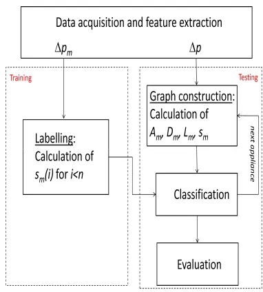
fidelity term is decreased. This iterative procedure stops once no improvement is observed. However, to keep the complexity low, in this paper, we only minimize the smoothness term. The flow chart of the algorithm is shown in Figure 1. During the training phase, sm(i) is determined for i < n, using

(2) based on the training dataset. The testing phase consists of constructing the graph and calculating s∗

m using (10) and

binary classification for each appliance. The summary of the algorithmic steps is given below.

Summary of the proposed algorithm.

1) For all appliancesm∈M¯

2) Calculate Lm using (5).

3) Calculate s∗

m using (10) and determinep∗m.

4) Remove the load of appliancemfrom the aggregate readings.

5) If there are remaining Appliance, then Go to Step 1. 6) Output:p∗

m for allm.

The complexity of the approach depends onN−nsince it is necessary to find the pseudo-inverse of an(N−n)×(N−n)

real-valued matrix, which can be done in O((N−n)3_{) time.}

∆

∆

%&' ()()*

%+, -()* . / 012 1 3 4 # $ $ 5 6 # 7

Fig. 1. Flow chart of the proposed algorithm.

Note that N−ncan be made as small as one (as done in the next section), in which case the decision is made as soon as the new sample is acquired.

IV. RESULTS ANDDISCUSSION

We present next our simulation results of low-rate energy disaggregation based on GSP and compare the performance to that of the state-of-the-art method of [11], which is based on HMM. Results of event-based approaches developed by authors are discussed in [4], [14], [32], where comparison with [11] is always provided. We use a dataset from the publicly available REDD database [18] downsampled to 1min resolution. For training we use M=200 samples, that is, just over three hours. For testing, we use 10,000 consecutive samples, which is almost a week worth of data.

The evaluation metrics used are precision (PR), recall (RE) and F-Measure (FM) [33] defined as:

P R=T P/(T P+F P) (11) RE=T P/(T P +F N) (12) FM = 2∗(P R∗RE)/(P R+RE), (13)

where true positive (TP) presents the correct claim the detected appliance was used, false positive (FP) represents an incorrect claim the appliance was not running, and false negative (FN) indicates that the appliance operation was not detected. Pre-cision captures the correctness of estimation - the higher the PR the few the FPs. On the other hand, high RE means a low number of FNs, which means that a higher percentage of power values are estimated correctly.FM balances PR and RE.

In the first simulation, we assess the performance of the algorithm without any base load and unknown appliances running. To avoid detecting stand-by settings, in this simu-lation, we set the threshold to T r =10W, that is, appliances operating below 10W are considered inactive - sm(i) = −1

For simplicity, we report results obtained purely by minimizing the smoothness term. We consider three appliances from House 2, namely, Refrigerator, Microwave, and Toaster, which were summed up to form an aggregated power signal p(i). Results are shown in Table I.

It can be seen from the table that the method was successful in disaggregating the toaster with only 6 FNs and no FPs. A worse performance for the microwave is due to the fact that often, the microwave was running only for a minute resulting in a single high power sample. Since, the methodology is based on maximizing smoothness of the signal, these events were sometimes missed. Moreover, the microwave operates at two different power levels (one around 50W and the other around 1900W), depending on the settings selected. The refrigerator iterates between the stand-by mode and the cooling up mode. The cooling-up mode was sometimes missed due to over-smoothing.

TABLE I. PERFORMANCE OF THE PROPOSED METHOD FOR THREE APPLIANCES.

Appliance TP FP FN PR RE FM Refrigerator 474 20 117 0.96 0.80 0.87

Toaster 98 0 12 1 0.89 0.94 Microwave 10 0 50 1 0.17 0.29

To demonstrate the performance in a real setting, we use House 2 dataset from the REDD database. House 2 contains 6 appliances: stove, toaster, refrigerator, microwave, dishwasher, and disposal. Since there were only two runs (1 minute each) of the disposal, this appliance was not considered. We disaggregate one appliance at the time, starting from highest consumers, and adaptively reducing the threshold. The results are shown in Table II. Similarly to the previous example, the disaggregation of the microwave suffers from low RE due to a high number of FNs. The number of FPs is high for the refrigerator and toaster mainly due to over-smoothing. Similar results can be observed from House 6 dataset, shown in Table III.

In the above experiments, we set N = M + 1 to reduce the complexity, to get an insight on practical implementation. The execution time was just over 2 msec per sample. This is roughly 4 times less than the average time needed for the HMM-based approach of [11] to disaggregate a sample. The programs were executed on Intel Core 2 CPU 2.66GHz machine running Windows XP and are coded in Matlab2014.

TABLE II. PERFORMANCE OF THE PROPOSED METHOD FORHOUSE2

FROM THEREDDDATASET.

Appliance TP FP FN PR RE FM Stove 19 54 1 0.26 0.15 0.41 Refrigerator 321 161 220 0.67 0.59 0.63 Toaster 93 111 20 0.41 0.82 0.59 Microwave 21 14 105 0.60 0.17 0.26 Dishwasher 7 10 1 0.41 0.88 0.56

Next, we compare the performance to that of the HMM-based method of [11]. Tables IV and V, show the results for the two methods, for House 2 and 6, respectively. In both houses, the HMM method disaggregates better the refrigerator. It is well known that HMM is successful in disaggregating the refrigerator due to regular cycles, continuous activities, sole

TABLE III. PERFORMANCE OF THE PROPOSED METHOD FORHOUSE6

FROM THEREDDDATASET.

Appliance TP FP FN PR RE FM Stove 4 0 0 1 1 1 Refrigerator 232 73 320 0.76 0.42 0.54

Toaster 2 0 0 1 1 1 Microwave 6 0 1 1 0.86 0.92

AC 59 108 16 0.35 0.79 0.49 Electric Heater 2 25 8 0.07 0.2 0.11

activities (i.e., without any other appliances running) during the night and hence huge data availability for learning and improving initial models [11], [4]. For all other appliances (except Microwave and Toaster in House 2), the proposed method shows better performance, at lower testing complexity. For example, HMM misses all uses of strove and microwave in House 6, while the proposed method has particularly high performance for disaggregation of these two appliances. One reason for low HMM performance for some appliances is short training period, which is not enough to build good initial appliance models.

The obtained results are comparable to other HMM-based methods, such as those of [12] and [34] that reported the total, ‘house-wise’FM for House 6 0.39 and 0.82, respectively (see

Table I in [34]).

V. CONCLUSION

In this paper, a novel approach for non-intrusive appliance load monitoring based on the emerging concept of graph signal processing was proposed. The proposed approach is not state based, avoiding common problems with conventional state-based NALM approaches, such as HMM state-based, related to high complexity and difficulties of designing efficient event detection. The optimization problem was formulated based on regularization on graph signals and a greedy algorithm was proposed. Experimental results using the publicly available REDD dataset demonstrate potentials of the approach and improved performance compared to the state-of-the-art HMM-based NALM method.

This paper has demonstrated the potential of using a graph-based signal processing approach for energy disaggregation. Future work will consist of testing the algorithm using different datasets, investigating other weight functions for adjacency matrix, assessing robustness of the algorithm with respect to noisy and incomplete training dataset, improving the perfor-mance by avoiding over-smoothing, and assessing near real-time testing performance.

ACKNOWLEDGMENT

TABLE IV. COMPARISON BETWEEN THE PROPOSED METHOD ANDHMM-BASED METHOD FORHOUSE2FROM THEREDDDATASET. Appliance PRp REp FMp PRHMM REHMM FMHM M

Stove 0.26 0.15 0.41 0.37 0.14 0.21 Refrigerator 0.67 0.59 0.63 0.88 0.92 0.90 Toaster 0.41 0.82 0.59 0.72 0.64 0.68 Microwave 0.60 0.17 0.26 0.33 0.84 0.47 Dishwasher 0.41 0.88 0.56 0.02 0.96 0.04

TABLE V. COMPARISON BETWEEN THE PROPOSED METHOD ANDHMM-BASED METHOD FORHOUSE6FROM THEREDDDATASET. Appliance PRp REp FMp PRHMM REHMM FMHM M

Stove 1 1 1 0 0.18 0 Refrigerator 0.76 0.42 0.54 0.95 0.82 0.88

Toaster 1 1 1 0 0.5 0 Microwave 1 0.86 0.92 0 0.78 0 AC 0.35 0.79 0.49 0.06 0.99 0.12 Electric Heater 0.07 0.2 0.11 0.02 0.91 0.03

REFERENCES

[1] G. W. Hart, “Nonintrusive Appliance Load Data Acquisition Method”,

MIT Energy Laboratory Technical Report, Sept. 1984.

[2] G. W. Hart, “Non-intrusive appliance load monitoring”, Proc. of the IEEE,vol. 80, no. 12, pp. 1870–1891, Dec. 1992.

[3] Government response to the consultation on the second version of the Smart Metering Equipment Technical Specifications: Part 2,Department of Energy & Climate Change UK, Dec. 2013.

[4] J. Liao, G. Elafoudi, L. Stankovic, and V. Stankovic, ”Power disag-gregation for low-sampling rate data,” 2nd International Non-intrusive Appliance Load Monitoring Workshop,Austin, TX, June 2014. [5] J. Liao, L. Stankovic, and V. Stankovic, ”Detecting household activity

patterns from smart meter data,” IE-2014 10th IEEE International Conference on Intelligent Environments,Shanghai, China, July 2014. [6] M. Zeifman and K. Roth, “Nonintrusive appliance load monitoring:

Review and outlook,”IEEE Transactions on Consumer Electronics, vol. 57, no. 1, pp. 76–84, Feb. 2011.

[7] A. Zoha, A. Gluhak, M.A. Imran, and S. Rajasegarar, “Non-intrusive load monitoring approaches for disaggregated energy sensing: A survey,”

Sensors,vol. 12, pp. 16838–16866, Dec. 2012.

[8] Y.F. Wong, Y.A. Sekercioglu, T. Drummond, and V.S. Wong, ”Recent approaches to non-intrusive load monitoring techniques in residential settings,” in Proc. CIASG-2013 IEEE Computational Intelligence Ap-plications in Smart Grids,Singapore, April 2013.

[9] T. Zia, D. Bruckner, and A. Zaidi, “A Hidden Markov Model based procedure for identifying household electric loads,” In Proc. IECON-2011 37th IEEE Annual Conference on Industrial Electronics Society,

Melbourne, Australia, Nov. 2011.

[10] H. Kim, M. Marwah, M. Arlitt, G. Lyon, and J. Han, “Unsupervised disaggregation of low frequency power measurements,” in Proc. 11th SIAM International Conference on Data Mining,Mesa, AZ, April 2011. [11] O. Parson, S. Ghosh, M. Weal, and A. Rogers, “Non-intrusive load monitoring using prior models of general appliance types,” inProc. the 26th Conference on Artificial Intelligence (AAAI-12), Toronto, CA, pp. 356–362, July 2012.

[12] J. Kolter, and T. Jaakkola, “Approximate inference in additive factorial HMMs with application to energy disaggregation,” in Journal on Machine Learning, vol. 22, pp. 1472–1482, 2012.

[13] S. Barker, S. Kalra, D. Irwin, and P. Shenoy, ”NILM redux: The case for emphasizing applications over accuracy,”2nd International Non-intrusive Appliance Load Monitoring Workshop,Austin, TX, June 2014. [14] H. Altrabalsi, J. Liao, L. Stankovic, and V. Stankovic, “A

low-complexity energy disaggregation method: Performance and robustness,”

SSCI-2014 IEEE Symposium on Computational Intelligence Applications in Smart Grid, Orlando, FL, December 2014.

[15] D. I. Shuman, S. K. Narang, P. Frossard, A. Ortega, and P. Van-dergheynst, ”The emerging field of signal processing on graphs: Ex-tending high-dimensional data analysis to networks and other irregular

domains,IEEE Signal Processing Magazine, vol. 30, no. 3, pp. 8398, May 2013.

[16] A. Sandryhaila and M.F. Moura, ”Discrete signal processing on graphs,”

IEEE Transactions on Signal Processing,vol. 61, pp. 1644–1656, July 2013.

[17] A. Sandryhaila and J. Moura, ”Classification via regularization on graphs, in Proc.Symposium on Graph Signal Processing in IEEE Global Conference on Signal and Information Processing (GlobalSIP), Austin, TX, December 2013.

[18] J. Kolter, and M. Johnson, “REDD: A public data set for energy disaggregation research,” in Workshop on Data Mining Applications in Sustainability (SIGKDD), San Diego, CA, 2011.

[19] W. Hu, G. Cheung, X. Li, and O. Au, ”Depth map compression using multi-resolution graph-based transform for depth-image-based rendering, in Proc.ICIP-2012 IEEE International Conference on Image Processing, Orlando, FL, September 2012.

[20] W. Hu, X. Li, G. Cheung, and O. Au, ”Depth map denoising using graphbased transform and group sparsity, in Proc. MMSP-2013 IEEE International Workshop on Multimedia Signal Processing, Pula, Italy, October 2013.

[21] C. Yang, Y. Mao, G. Cheung, V. Stankovic, and K. Chan, ”Graph-based depth video denoising and event detection for sleep monitoring,” in Proc.MMSP-2014 IEEE International Workshop on Multimedia Signal Processing,Jakarta, Indonesia, Sept. 2014.

[22] G.Y. Lin, S.C. Lee, Y.J. Hsu, and W.R. Jih, ”Applying power meters for appliance recognition on the electric panel,”in Proc. the 5th IEEE Conference on Industrial Electronics and Applications, pp. 22542259, Melbourne, Australia, June 2010.

[23] Y.X. Lai, C.F. Lai, Y.M. Huang, and H.C. Chao, ”Multi-appliance recognition system with hybrid SVM/GMM classifier in ubiquitous smart home.,”Inform. Sci.2012.

[24] T. Kato, T, H.S. Cho, and D. Lee, ”Appliance recognition from electric current signals for information-energy Integrated network in home environments,” in Proc. 7th International Conference on Smart Homes and Health Telematics, vol. 5597, pp. 150–157, Tours, France, July 2009.

[25] D. Srinivasan, W. Ng, and A. Liew, ”Neural-network-based signature recognition for harmonic source identification,”IEEE Transactions on Power Deliverypp. 398–405, vol. 21, Jan. 2006.

[26] A. G. Ruzzelli, C. Nicolas, A. Schoofs, and G.M.P. O’Hare, “Real-time recognition and profiling of appliances through a single electricity sensor, ”IEEE SECON-2010 7th Annual Conf. Sensor Mesh and Ad Hoc Communications and Networks, pp.1–9, Boston, June 2010.

[27] M. Berges, E. Goldman, H. S. Matthews, and L. Soibelman, “Learning systems for electric consumption of buildings,” in Proc. 2009 ASCE International Workshop on Computing in Civil Engineering, Austin, TX, 2009.

Inter-national Conference on Ubiquitous Intelligence and Computing and 9th International Conference on Automatic and Trusted Computing, 2012. [29] M.J. Johnson and A.S. Willsky, “Bayesian nonparametric Hidden

Semi-Markov Models,”Journal on Machine Learning Research (JMLR), vol. 14, pp. 673–701, Feb. 2013.

[30] S. Markonin, I.V. Bajic, and F. Popowich, ”Efficient sparse matric processing for nonintrusive load monitoring,” 2nd International Non-intrusive Appliance Load Monitoring Workshop,Austin, TX, June 2014. [31] S. Boyd and L. Vandenberghe,Convex Optimization,Cambridge, 2004. [32] J. Liao, G. Elafoudi, L. Stankovic, and V. Stankovic, “Non-intrusive appliance load monitoring using low-resolution smart meter data,” Smart-GridComm IEEE International Conference on Smart Grid Communica-tions, Venice, Italy, November 2014.

[33] D.L. Olson and D. Delen, Advanced Data Mining Techniques, Springer, 2008.