Framework for the Buckling Optimization of Variable-Angle
Tow Composite Plates
Zhangming Wu,∗Gangadharan Raju,†and Paul M. Weaver‡ University of Bristol, Bristol, England BS8 1TR, United Kingdom
DOI: 10.2514/1.J054029
Variable-angle tow describes fibers in a composite lamina that have been steered curvilinearly. In doing so, substantially enlarged freedom for stiffness tailoring of composite laminates is enabled. Variable-angle tow composite structures have been shown to have improved buckling and postbuckling load-carrying capability when compared to straight fiber composites. However, their structural analysis and optimal design is more computationally expensive due to the exponential increase in number of variables associated with spatially varying planar fiber orientations in addition to stacking sequence considerations. In this work, an efficient two-level optimization framework using lamination parameters as design variables has been enhanced and generalized to the design of variable-angle tow plates. New explicit stiffness matrices are found in terms of component material invariants and lamination parameters. The convex hull property of B-splines is exploited to ensure pointwise feasibility of lamination parameters. In addition, a set of new explicit closed-form expressions defines the feasible region of two in-plane and two out-of-plane lamination parameters, which are used for the design of orthotropic laminates. Finally, numerical examples of plates under compression loading with different boundary conditions and aspect ratios are investigated. Reliable optimal solutions demonstrate the robustness and computational efficiency of the proposed optimization methodology.
Nomenclature
A = matrix of in-plane stiffness (Aij) a,b,h = length, width, and thickness of plate Brsx,Brsy = xandycoordinates of control points
for a B-spline
cj = undetermined weight for a component of in-plane force loading
D = matrix of bending stiffness (Dij) Eiso,νiso,Diso = equivalent Young’s modulus, Poisson’s
ratio, and bending stiffness of quasi-isotropic laminate e = test variable in the trial functiong F = vector of applied in-plane loading f,g = trial functions for Schwarz inequality
fi = objective function or constraint function HL,HU = lower and upper bounds of each
hyperplane constraint
h = fh1; h2; h3; h4; h5g; vector for a
hyperplane along the boundary of the feasible regions K
cr = normalized buckling load of
variable-angle tow plate Kb
0,Kb1,Kb2 = separate parts of bending stiffness matrix
Ks
10; Ks11;· · · = separate parts of stability stiffness matrix
Kb,Ks = bending stiffness matrix and stability matrix in buckling model
Km = in-plane stiffness matrix in prebuckling model
k,Ξ = order (degree) and knot vector of B-splines
N,M = in-plane stress and bending moment resultants
Nsk,Nsk = B-spline basis functions
Ncr
xiso = critical buckling load of quasi-isotropic laminate
Ncr
xvat = critical buckling load of variable-angle tow laminate
R = plate aspect ratio (a∕b)
s,t = directional variables for a general parabola
Tmn = fiber angle of variable-angle tow plate at a control point (Pmn)
U = vector of unknown coefficients for in-plane displacements
Upq,Vpq,Wpq = undetermined coefficients for displacement fields
U1,U2,U3,U4,U5 = material invariants
u0 = prescribed in-plane displacement loading
u0,v0 = in-plane displacement at reference plane
inxandydirections
u,v = B-spline parametric coordinates
w = out-of-plane deflection
wA i,w
D
i = weighting functions
Xux,Yuy = shape functions for in-plane displacementu0
Xvx,Yvy = shape functions for in-plane displacementv0
Xwx,Ywy = shape functions for out-of-plane displacementw
z,z = direction along the thickness of a laminate
zx,zy = distance of a ply to the midplane
αμ,βμ = upper and lower moving asymptotes Γ,Γrsτ = lamination parameters at a control
point (Prs)
Δx = end-shortening displacement along xdirection
ϵ0,κ = midplane strains and out-of-plane
curvatures Received 25 November 2014; revision received 5 May 2015; accepted for
publication 26 May 2015; published online 30 July 2015. Copyright © 2015 by Z. Wu, G. Raju, and P. M. Weaver. Published by the American Institute of Aeronautics and Astronautics, Inc., with permission. Copies of this paper may be made for personal or internal use, on condition that the copier pay the $10.00 per-copy fee to the Copyright Clearance Center, Inc., 222 Rosewood Drive, Danvers, MA 01923; include the code 1533-385X/15 and $10.00 in correspondence with the CCC.
*Postdoctoral Researcher, Advanced Composite Centre for Innovation and Science, Department of Aerospace Engineering, Queen’s Building, University Walk.
†Research Assistant, Advanced Composite Centre for Innovation and
Science, Department of Aerospace Engineering, Queen’s Building, University Walk.
‡Professor in Lightweight Structures, Advanced Composite Centre for
Innovation and Science, Department of Aerospace Engineering, Queen’s Building, University Walk. Member AIAA.
Article in Advance / 1
θx; y = variation of fiber angle of a variable-angle tow layer
λ(λcr) = eigenvalue of buckling model
μ,ν = indices of the outer and inner iterations in a globally convergent method of moving asymptotes routine
ξA
1,ξ
A
2 = in-plane lamination parameters ξD
1,ξ
D
2 = out-of-plane lamination parameters
τ = 1(ξA
1), 2(ξ
A
2), 3(ξ
D
1), and 4(ξ
D
2)
Ψx;y = general shape function
I. Introduction
A
DVANCED tow placement techniques allow the fiber (tow) to be placed curvilinearly within a lamina and, in doing so, enable the designer to take advantage of the directional properties of com-posite laminates. The concept of tow steering can be applied to the design of lightweight structures with potentially enhanced perfor-mance for aerospace applications [1–4]. In the preliminary design of long and slender aerospace structures, buckling resistance is often considered as a primary design criterion. It has been reported pre-viously that the buckling load-carrying capacity of variable-angle tow (VAT) plates can be substantially improved when the in-plane prebuckling stresses that result from the variable stiffness are redistributed beneficially [2,3,5]. In contrast to the benefits offered by VAT, the optimal design of VAT laminates is a difficult task to undertake due to the increased design choice available to the designer for pointwise stiffness tailoring. The design of VAT laminates involves a large number of variables, as one has to determine the layup sequence at each point in the structure. The aim of this work is to develop a rapid, yet efficient, optimization framework to design VAT composite plates for maximum buckling load.Ghiasi et al. [6] presented a thorough review of different opti-mization techniques for the design of variable stiffness composite plates, in which it was concluded that the multilevel optimization method is recommended due to its highly computational efficiency. Setoodeh et al. [7] used a reciprocal approximation method to design VAT plates for maximum buckling load and used finite element nodal fiber angles as design variables. Wu et al. [3] proposed a general control-point design scheme to describe a continuous variation of fiber angles, where the VAT configuration was optimized for maxi-mum buckling load. However, the objective function in terms of fiber angle or fiber trajectory was highly nonconvex and the opti-mization process was likely to get trapped in local optima. To over-come these problems, the approach of using lamination parameters as design variables was shown to be an effective way to solve the optimization problem of variable stiffness laminates [5,8]. Lami-nation parameters [9] are evaluated by integrating the trigonometric functions of the ply orientation across the thickness of the plate. Usage of lamination parameters to represent composite layups not only results in a reduction of design variables but also offers possibly the largest convex design space. In addition, an optimization process can focus on the design of stiffness properties irrespective of laminate configuration (stacking sequence and fiber orientations). The advantage of using lamination parameters over using ply angles as design variables to perform the optimal design of constant-stiffness composite laminates has been reported in previous works [10–12]. The primary benefit arises from representing laminate stiffness as linear combinations of both material invariants and lamination parameters, which can lead to convex design spaces that enable efficient gradient-based optimizers to find global optima. Lamination parameters have also been successfully applied to the design of variable stiffness composite structures. Setoodeh et al. [13] and Abdalla et al. [14] optimized the in-plane stiffness and natural frequency of variable stiffness plates using lamination parameters, respectively. Ijsselmuiden et al. [5,15] presented a sophisticated framework based on finite element modeling and a successive approximation optimization technique [16] to perform the design of variable stiffness structures for maximum buckling load. All of these works [5,14,17] rely on a finite element design scheme, in which the local lamination parameters (design variables) are piecewise constant
and associated with each element/node. However, the element-based optimization method may suffer from the increasing number of design variables and nonsmooth distribution of the lamination parameters unless an additional smoothing constraint is applied.
Furthermore, the values of 12 lamination parameters are not completely independent and are linked by a particular layup. Con-straints that define the design space (feasible region) of lamination parameters are needed for an optimization process. Currently, the closed-form expressions that can exactly define the complete feasible region of 12 lamination parameters remain unknown. Miki and Sugiyama [10] first derived the parabolic relation of two in-plane or two out-of-plane lamination parameters. Later, Fukunaga and Sekine [18] further obtained closed-form expressions that could represent the feasible regions of the four in-plane and four out-of-plane lamination parameters. The pioneering work of Grenestedt and Gudmundson [19] proved the convexity of the feasible region of lamination parameters (also for the case of variable stiffness) and proposed a variational approach to evaluate the feasible region numerically. In the design of VAT laminates, the value of each lamination parameter varies continuously across the planform and the corresponding feasibility constraints should be satisfied at every point. Hence, an accurate bound for the feasible region of lamination parameters is necessary in the design of VAT laminates. Setoodeh et al. [20] proposed a convex hull approach to numerically represent the feasible region in terms of a large number (37,126) of linear algebraic equations (hyperplanes). Based on Bloomfield et al.’s work [21], we derive a small number of new explicit nonlinear expressions that give a relatively accurate boundary for the feasible region of these four lamination parameters, which is sufficient to define orthotropic VAT laminates.
The main objective of this paper is to introduce an optimization framework that employs B-splines to define the spatial variation of lamination parameters (variable stiffness). B-spline or nonuniform rational B-spline (NURBS) techniques that have been widely used in CAD systems [22] are able to represent complex geometries (variations) using relatively few design variables. A given degree B-spline curve/surface is determined by a set of control points and a prescribed knot vector. The control points are distributed over the plate domain, and the design variables (lamination parameters) are associated with each control point. The design flexibility is adjusted by altering the number and position of control points, the degree, and the knot vector of spline functions. This approach of defining the spatial variation ofA,Dstiffness matrices using B-spline functions is inspired by isogeometric analysis [23,24]. However, we do not need the complexity of NURBS functions and limit our choice to B-splines to represent lamination parameter variation because we only exploit the smoothness and convex properties. Compared with the dis-cretized finite element approach, using B-splines to represent the spatial variation of lamination parameters requires less design variables and leads to a continuous and smooth distribution. In ad-dition, the convex hull property of B-splines enforces the spatially varying lamination parameter across the planform of the plate to be fully constrained inside the feasible region, provided that the lamination parameters at the control points satisfy all the nonlinear constraints. Using B-splines avoids the problem of satisfying a large number of feasibility constraints at an infinite number of points in the plate that results in a cumbersome semi-infinite programming pro-blem. In recent work, isogeometric techniques [25] have been applied to model and design VAT laminates with B-spline (or NURBS) format stiffness variation using finite element analysis as the structural tool. Our approach uses a more computationally efficient structural model than shown in [3], but it is not as versatile for complex geometries. In addition, we decouple the discretization scheme for the design of VAT layers from the structural modeling of VAT plates. However, the finite element approach including the isogeometric technique adopts the same discretization scheme for both the design and the structural model. Such an approach is efficient only where the optimal mesh size for structural analysis is the same as that needed for design and optimization. In our experience, we do not require as refined a mesh for optimization as is needed for analysis,
allowing us to use control-point variables used in optimization to be more sparsely distributed than that in the structural mesh.
For buckling or vibration optimization problems, the objective function expressed in terms of lamination parameters is much less ill conditioned (and can often be convex [19]) than using layer angles as the design variables. The revised objective function together with the convex design space reduces the complexity and computational time/ efforts effectively. In this work, a gradient-based algorithm called the globally convergent method of moving asymptotes (GCMMA) [26] is adopted. The GCMMA employs a successive convex ap-proximation technique, in which the objective functions and nonlinear constraints are replaced by a sequence of conservative convex separable approximations (subproblem) based on gradient information, and these subproblems are created and solved iteratively until a desired convergence is achieved. The approximation concept, introduced by Schmit and Farshi [27] and Schmit and Miura [28], has been extensively studied [29] and is a well-established technique for structural optimization. In previous works, the first-order Taylor series expansion [30], a reciprocal approximation [31], or a mixed-variable linearization were successively introduced to approximate the nonlinear objective/constraint functions at a local design point. The mixed-variable approach is more conservative than the former two methods, and it is a convex problem that can be readily solved by dual methods [32]. Later, Svanberg [33] developed a new method, named the method of moving asymptotes (MMA), for the convex and conservative approximation that could stabilize the optimization process through using two artificial asymptotes. The MMA was further developed for yielding a global convergent solution and is named GCMMA. In a GCMMA, additional damping factors are introduced to ensure a strict convexity of subproblems and the conservativeness is further checked iteratively.
In the current work, the buckling optimization of VAT plates is carried out within an enhanced two-level strategy, which advances the optimization framework first proposed by Yamazaki [34] and further developed by Diaconu and Weaver [35], Herencia et al. [36], and Bloomfield et al. [37] for straight fiber composites. At the first step, structural analysis is conducted using a Rayleigh–Ritz method in which novel explicit expressions for plate-level stiffness matrices were written in terms of component material invariants and lami-nation parameters. The spatially varying laminate stiffness, and therefore lamination parameter, distribution of VAT plates was represented using B-splines. Subsequently, a gradient-based method (GCMMA) was used to determine the optimal lamination parameters at each control point for the maximum buckling load. The con-vergence of the optimization process was studied by gradually increasing the number of the control points. Note, that the convexity of B-splines between control points guarantees feasibility of VAT layups if feasibility constraints on the lamination parameters have been satisfied at the control points. It is for this reason we choose B-splines to represent lamination parameter variation across the domain. At the end of the first step, we recover a smooth, continuous variation of lamination parameters that satisfies feasibility constraints on their values. At the second step, smooth, spatially varying dis-tributions of fiber-orientation angles are retrieved from the target lamination parameters using a genetic algorithm (GA) in a similar way to that done previously [34,35]. The two-level approach pro-vides an efficient way to solve the optimization problem, especially for VAT laminates. Furthermore, the lamination parameters guided design process allows the best possible laminate configuration to be determined, both theoretically (first-level) and that can be realized (second-level). The proposed optimization framework for the design of VAT laminates is used subsequently to determine the optimal fiber angle distribution for maximizing the buckling performance under different boundary conditions and loading cases.
II. Lamination Parameters A. Definition of Lamination Parameters
Considering classical lamination theory, the constitutive equation of a VAT plate is given by
N M
Ax;y Bx; y
BTx; y Dx;y
ϵ0
κ
(1)
The in-plane, coupling, and bending stiffness matrices are functions ofxandyfor VAT plates, denoted byAx;y,Bx; y, and Dx;y, respectively. The stiffness matrices are expressed as a linear combination of lamination parameters and material invariants. In the present study, only specially orthotropic VAT laminates are con-sidered. In other words, there are no in-plane and out-of-plane couplings (B0), no extension-shear coupling (A160,A260),
and no flexural-twisting coupling (D160,D260). As a result,
two in-plane and two out-of-plane lamination parameters are sufficient to define the stiffness matrices as
0 B B B @ A11 A22 A12 A66 1 C C C Ah
2 6 6 6 4
1 ξA
1 ξA2 0 0
1 −ξA
1 ξ
A
2 0 0
0 0 −ξA
2 1 0
0 0 −ξA
2 0 1 3 7 7 7 5 0 B B B @ U1 U2 U3 U4 U5 1 C C C A (2) 0 B B B @ D11 D22 D12 D66 1 C C C A h3 12 2 6 6 6 4
1 ξD
1 ξD2 0 0
1 −ξD
1 ξD2 0 0
0 0 −ξD
2 1 0
0 0 −ξD
2 0 1
3 7 7 7 5 0 B B B @ U1 U2 U3 U4 U5 1 C C C A (3)
where the four lamination parameters are defined by
ξA
1;2
1 2
Z1
−1
cos2θzcos4θzd z
ξD
1;2
3 2
Z1
−1
cos2θzcos4θzd z (4)
whereθzis the layup function in the thickness direction of the plate.
B. Feasible Region of Lamination Parameters
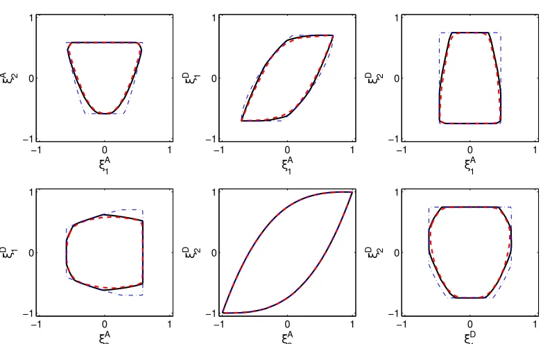
The entire distribution of spatial variable stiffness of the VAT laminates are not independent of each other; and their feasible region, in terms of lamination parameters, forms a convex space [19]. Their values are required to be strictly constrained inside the feasible region to ensure a stable optimization procedure for the design of VAT laminates. An accurate boundary of the feasible region of lamination parameters is then important for the optimization of VAT laminates. Grenestedt and Gudmindson [19] presented a set of equations that gave an outer boundary for the feasible region of lamination pa-rameters. In the current work, we derive a set of new explicit closed-form expressions that accurately defines the interdependent feasible region ofξA
1;2andξ
D
1;2. The derivation of these equations is given in
Appendix A. The nonlinear constraints for these four coupled lamination parameters are given by
5ξA
1−ξD12−21ξA2−2ξA12≤0 (5)
ξA
2−4tξA112t23−412jtjt22ξD2−4tξD112t2≤0
(6)
4tξA
1−ξA214jtj3−412jtjt224tξD1−ξ2D14jtj≤0
(7)
where t −1;−0.75;−0.5;−0.25;0;0.25;0.5;0.75;1 (or, for better accuracy, t −1;−0.8;−0.6;−0.4;−0.2;0;0.2;0.4;0.6; 0.8;1). These19∼23equations in Eqs. (5–7) are able to accurately bound the feasible region of the four lamination parametersξA;D1;2, as shown in Fig. A2.
III. Buckling Analysis
Before buckling analysis, the nonuniform load redistribution of in-plane stress resultants of VAT plates that arises in response to stiffness variations is required [2,38]. Here, both the prebuckling and buckling problems are solved using a Rayleigh–Ritz procedure through the minimization of potential energy (or complementary energy).
To take advantage of the linear relations, as shown in Eqs. (2) and (3), between the stiffness matrices (A,D) and the lamination parameters (ξA;D1;2), the VAT plate is modeled in terms of displacement
fields, each of which is expanded into an independent series:
u0x; y X
P1
p
XQ2
q
UpqXupxYuqy;
v0x; y X
P2
p
XQ2
q
VpqXvpxYvqy;
wx; y X
M
m
XN
n
WmnXwmxYwny (8)
whereUpq,Vpq, andWmnare undetermined coefficients for three displacement components u0x; y, v0x; y, andwx; y,
respec-tively. The shape functionsXu
px; Yuqx;· · ·; Ywnx in the series expansions must satisfy geometric boundary conditions on the edges. By substituting the series expansions ofu0x; yandv0x; yin
Eq. (8) into the potential energy, the in-plane stretching problem of VAT plates under a prescribed force loading is solved and given by [39,40] as
Πs1
2
Z Z
A11 ∂
u0 ∂x
2 2A12
∂
u0 ∂x
∂v0 ∂y
A22
∂
v0 ∂x
2
A66 ∂
u0 ∂y
∂v0 ∂x
2
dxdy−
Z
C1
NxνuNyνvds (9)
where Nxν and Nyν are in-plane boundary stress resultants. The prebuckling problem of a VAT plate under prescribed loading is modeled as a linear algebraic problem, which is expressed in matrix form as
Km·UF (10)
whereUis a vector of the undetermined coefficients (Upq VpqT) from the in-plane displacement fields u0x; y and v0x; y. The
vectorFis associated with the prescribed in-plane loading. Note that, using Eq. (10) to directly model a VAT plate subjected to prescribed displacement boundary conditions u0 (i.e., an end-shortening
displacement compression), is generally difficult to achieve, as the boundary forces are nonuniform and unknown [38]. As prebuckling is a linear elasticity problem, the superposition principle is applied. As such, the prebuckling problem of a VAT plate under a prescribed displacement loadingu0is modeled as a superposition of the VAT
plates under a series of given nonuniform boundary stress loading conditions. Equation (10) is then rewritten as
Km·U
jFj (11)
where the vector Fj denotes applied boundary force, which is assumed to be constant, linear, parabolic, cubic, and higher-order variations forj0;1;2;· · · . The prebuckling model of a VAT plate under prescribed displacement loading is then expressed as a sum of a series of the solution of Eq. (11) with undetermined weightscj:
X
j
cjKm·Uj
X
j
cjFj⇒ Km·
X
j cjUj
X
j
cjFj (12)
where the coefficientscjare determined by satisfying the boundary conditionsu0
X
j cjUj
·ψxjxxju0 (13)
andψxdenotes a vector of in-plane shape functionsXu
pxYuqyT (orXv
pxYvqyT), andxj xj; yjis a selected grid point along the boundary edges where the boundary conditionsu0are applied.
Subsequently, the nonuniform stress fields are obtained from the constitutive equation as
NA·ϵ0A·Dux A·Dψx·X
j
cjUj (14)
By substituting the transverse deflectionwx; yinto the potential energy for bending of VAT plates [38], the buckling analysis is expressed as the following eigenvalue problem:
fKb−λKsgfwg 0 (15)
Note that different approaches (finite element method, the finite difference method, and differential quadrature method [41]) have been used to model the prebuckling and buckling behaviors of VAT plates, resulting in the same matrix formulas as Eqs. (11) and (15). The optimization methodologies presented in subsequent sections are applicable to other modeling approaches. Of these, the Rayleigh– Ritz (or Galerkin) method has the advantage that it requires relatively little computational cost and allows sensitivities to be calculated analytically.
IV. Two-Level Optimization Strategy
The buckling optimization procedure of VAT plates is split into two steps. At the first step, a gradient-based mathematical programming technique is used to determine the optimum dis-tribution/variation of lamination parameters, which gives the maxi-mum buckling load. At the second step, a GA is employed as an optimizer to obtain the actual layups (stacking sequence and fiber orientations) from the target value of lamination parameters.
A. First-Level Optimization
1. B-Spline Spatial Variation of Lamination Parameters
The distribution of four lamination parameters ξA;D1;2 for establishing an orthotropic VAT laminate configuration is rep-resented in terms of the B-spline surface as
xu; v X r
X
s BrsxN
k
r uN k
s v
yu; v X r
X
s
BrsyNrkuNskv
ξA;D
1;2u; v X
r
X
s Γτ
rsNrkuNskv (16)
where the values ofBrsx and Brsy represent the location of each predefined control pointPrs(as shown in Fig. 1) along thexandy axes, respectively. The coefficientΓrsτin Eq. (16) is the assigned value of a particular lamination parameter at each predefined control point Prs. The term τ1;2;3, and 4 denotes four different lamination parametersξA
1,ξ
A
2,ξ
D
1, andξ
D
2, respectively. The B-spline
basis functionNrku [or Nskv] is akth order (k−1degree) piecewise polynomial that is determined by a defined knot vectorΞ. When the lamination parameters (stiffness) are defined to vary along one principal direction (for example, they axis), the variation is defined by the B-spline curve:
yv X
s
BsyNskv ξA;D1;2v
X
s Γτ
[image:4.585.39.280.357.409.2]s Nskv (17)
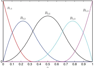
Figure 1 demonstrates an example of using the B-spline surface with 5-by-5 (25) uniformly spaced control points to construct the distribution of lamination parameters varying along both thexandy axes. The order and the knot vector for the B-splines in this example
are chosen to bek3andΞ 0;0;0;1∕3;2∕3;1;1;1(uniform), respectively. Figure 2 shows the open uniform B-spline basis functions, which are piecewise quadratic polynomials. The optimal design is performed by adjusting the values of the lamination parameters (ξA;D1;2) at the 25 control points, and this approximation
does not represent the complete design space. However, increasing the number of control points ensures greater convergence of the complete design space.
B-splines possess several special features, which make them suitable for representing the spatial variation of lamination pa-rameters of VAT laminates. Using B-splines generally results in continuous and smooth distributions, with the degree of local variation specified byk. The plate domain is subdivided into a grid that consists of a series of patches, and the B-splines are defined locally over each patch. The local support property of B-spline controls the variation within each patch, i.e., adjusting the value of a control point only affects variation inside the local patch. This feature is particularly useful for the concept of local stiffness tailoring and offers the possibility of implementing a tool for both modeling and optimization of blended VAT laminates. Another desirable feature of splines is their strong convex hull property, which states that a B-spline surface is strictly constrained in the convex hull formed by its control polygon. This convex hull property enables the entire dis-tribution of the lamination parameters to be constrained strictly inside the feasible region by satisfying the nonlinear constraints defined in Eqs. (5–7) at the control points. Using other algebraic polynomial functions (but without the convex hull property) leads to a semi-infinite programming problem in the optimization of VAT laminates. Solving a semi-infinite programming problem is highly computa-tionally expensive and may cause the optimization procedure to be numerically unstable.
Using higher-degree B-spline basis functions [for instance, the cubic variation (k4)] offers more local flexibility for the design of variable stiffness. However, it also limits the usage of design space
compared to quadratic variation. Applying the nonuniform rational B-splines to represent the variation of lamination parameters pro-vides larger design space and more design options (local refinement) than using the B-splines, as NURBS introduces a weighting coefficient (four-dimensional space) to each control point. However, the NURBS-based approach may considerably raise the difficulty of evaluating the sensitivities and the computational cost of opti-mization. As the plane domain of a VAT plate is smoothly varying, it is appropriate to use uniform basis functions and uniform-spaced control points to represent its stiffness variation. We anticipate that nonuniform basis functions and control points are better suited for the design of VAT laminates with cutouts and discontinuities.
As the stiffness variation (lamination parameters) of VAT plates is defined in a B-spline parametric spaceu; v[Eq. (16)], all the integra-tions involved in the prebuckling and buckling models [Eqs. (11–15)] defined over the plate domain x; y have to be transformed and evaluated in the B-Spline parametric domain. For example,
Z
ΩA11x; y·Ψx; ydxdy
Z
Ω
A11u; v
·Ψxu; v; yu; vJuvd ud v (18)
whereΨx; ydenotes a shape function that is employed in the model. The termsΩandΩ represent the integral domain underx; yand u; vcoordinates, respectively; andJuvis the Jacobian matrix for the
coordinates transformation. Equation (18) is further expanded in terms of lamination parameters as
Z
Ω
A11u; v·Ψ~u; vJuvd ud vh
U0 Z
Ω ~
Ψu; vJuvd ud v
X
rs
U1Γ 1
rs U2Γ 2
rs
Z
Ω
NrkuN k
s vΨ~u; vJuvd ud v
(19)
On the right-hand side of Eq. (19), the integrals are independent of material properties, plate dimensions, and the design variables (Γ1
rs, Γ2
rs). All of the other integrations in the prebuckling and buckling models are also transformed and expanded in a similar way to Eqs. (18) and (19). The numerical computation of these integrals, which is the most time consuming of the proposed design framework but only needs to be performed once in the whole optimization process. Furthermore, due to the local support property of B-spline basis function,Nrku and Nskv are nonzero only at a local region
tr; trk(ts; tsk). Each individual integration, for example,
Z
Ω
NrkuNskvΨ~u; vJuvd ud v Zt
rk tr
Zt sk ts
NrkuNskvΨ~u; vJuvd ud v (20)
is evaluated over a local B-spline patch.
Fig. 1 Illustration of B-spline surface constructing by five-by-five uniformly spaced control points.
Fig. 2 Uniform B-spline basis functions for N5, k3 and Ξ 0;0;0;1∕3;2∕3;1;1;1.
[image:5.585.126.458.47.221.2] [image:5.585.70.253.604.736.2]2. Sensitivity
The numerical accuracy of sensitivity information plays an important role in a gradient-based optimization routine. The buckling analysis of VAT plates is a conventional eigenvalue problem, and the sensitivity of the critical buckling load with respect to each design variable (lamination parameters at each control point) is evaluated as [42]
dλ
dΓrsτ
wT
dKb
dΓrsτ
−λdKs
dΓrsτ
w
(21)
where the buckling mode shape is normalized aswTKsw1. As illustrated by Eq. (19), the matrices (KbandKs) are separable with respect to design variables (lamination parameters). Hence, the matricesKbandKsare further expanded and written in the following form:
KbKb
0 X
rs Γ3
rsKb1
X
rs Γ4
rsKb2 (22)
KsX pq
UpqKs10 X
pq
X
rs
UpqΓrs1Ks11 X
pq
X
rs
UpqΓrs2Ks12
X
pq
VpqKs20 X
pq
X
rs
VpqΓrs1Ks21 X
pq
X
rs
VpqΓrs2Ks22 (23)
whereKb
0; Kb1;· · ·; Ks22 on the right-hand side of Eq. (23) are the
separated parts of the stiffness and stability matrices, which are functions of material invariants and B-splines (at each control point). In Eq. (22), the matrixKb
0is independent of design variables. The
matrices Kb
1 and K
b
2 are related to the out-of-plane lamination
parameters ofξD
1 andξ
D
2 at each control point (Prs), respectively. The stability matrix Ks is related to both in-plane lamination parameters and in-plane displacement fieldsUp; VpT(prebuckling solution). For the matricesKs
10; Ks11;· · ·; Ks22in Eq. (23), the number
in their subscripts (10;11;· · ·;22) specifies the relation of the corresponding matrix to the design variables and in-plane dis-placement fields. The first index in each subscript (1 or 2) indicates that the matrix is associated withu0orv0displacement fields. The
second index (0, 1, 2) in each subscript denotes the corresponding matrix is independent of design variables (equal to zero), associated withξA
1(equal to one) andξA2(equal to two), respectively. All of the
explicit expressions of these matrices in the Appendix B.
As previously mentioned, in Eqs. (22) and (23), the integrals involved inKb
0; K
b
1;· · ·; K
s
22are independent of the design variables
and are only evaluated once in an optimization process. The sensitivities in Eq. (21) are computed analytically based on the value of these matrices, and so improve the efficiency of the gradient-based optimization process. Due to the linear relationship between the bending stiffness matrix and the out-of-plane lamination parameters, the derivative ofKbin Eq. (21) is evaluated separately as
dKb
dΓrs3
Kb
1;
dKb
dΓrs4
Kb
2 (24)
On the other hand, a local change of in-plane stiffness may affect the entire in-plane stress distribution (prebuckling solution) [5]. The sensitivity evaluation of the stability matrixKsis related (coupled) to each component (Up,Vp) of the series expansion of the in-plane displacement field as
dKs
dΓrs1
X
pq
dU
pq
dΓrs1 Ks
10
dUpq
dΓrs1 Γ1
rsKs11UpqKs11
dUpq
dΓrs1 Γ2
rsKs12
X
pq
dV
pq
dΓrs1 Ks
20
dVpq
dΓrs1 Γ1
rsKs21VpqKs21
dVpq
dΓrs1 Γ2
rsKs22
(25)
dKs dΓrs2
X
pq
dU
pq
dΓrs2 Ks
10
dUpq
dΓrs2 Γ1
rsKs11UpqKs12
dUpq
dΓrs2 Γ2
rsKs12
X
pq
dVpq
dΓrs2 Ks
20
dVpq
dΓrs2 Γ1
rsKs21VpqKs22
dVpq
dΓrs2 Γ2
rsKs22
(26)
The derivatives of the in-plane displacement fields UUp VpTare determined from the prebuckling model as
dU
dΓrsτ
X
j
dc
j
dΓrsτ Ujcj
dUj
dΓrsτ
τ1;2 (27)
dcj
dΓrsτ
−U0−1dU0
dΓrsτ
cj τ1;2 (28)
dUj
dΓrsτ
−Km−1dK
m
dΓrsτ
Uj τ1;2 (29)
whereU0denotes the expression forψxUkjxx0.
Besides the sensitivities of buckling load, it is also necessary to obtain the gradient information of the nonlinear constraint functions (feasible region of lamination parameters), which is done readily from the expressions given in Eqs. (5–7).
3. Gradient-Based Optimization
The buckling load of a VAT plate is a function of both in-plane stiffness and bending stiffness λcrλA; D [2,3] due to the nonuniform in-plane stress fields. It was observed that the buckling load is a linear homogeneous function with respect to the bending stiffness. The in-plane stresses are linear functions of the reciprocal of the in-plane complianceA−1and proportional to the external applied
boundary force (displacement) [3]. Also, varying the amplitude of in-plane stresses does not affect the buckling eigenvalue (zero-order homogeneous property [5]), and only the stress distribution affects the buckling load. Therefore, the in-plane stiffness of VAT laminates has to be optimized to achieve a benign stress distribution that improves their buckling performance [2,3,5].
From our physical understanding, the improvement in buckling performance is mainly governed by the stress redistribution of loads from the center to the edges where the plate is supported. For straight fiber composites, the sensitivity of curvature plays a prominent role in improving the buckling performance, as it is governed by bending action of the plate. However, for VAT laminates, the buckling performance is governed by both stretching and bending behaviors. For VAT plates that are under axial compression loading conditions, the sensitivity of strains at both the domain and the boundary is equally important in redistributing the loads from the center toward the supported edges.
The sensitivity analysis [Eqs. (21–28)] shows that the buckling load is nonlinear with respect to each component of the in-plane stiffness matrixAij. The distributions of in-plane stiffness and the bending stiffness cannot vary independently and are linked by the values of material invariants and lamination parameters in a convex feasible space. Hence, the buckling design of VAT plates is a coupled nonlinear optimization problem in terms of stiffness matrices expressed using lamination parameters and requires nonlinear constraints to define the feasible region of lamination parameters. The first-level optimization of VAT plates for the maximum buckling load using lamination parameters is formulated as
min −λcrΓrsτ subjected to : −1⩽Γrsτ⩽1 giΓrsτ⩽0 (30)
The nonlinear constraint functions giΓ
τ
rsdefine the relations between the four different lamination parameters, given by
Eqs. (5–7). The satisfaction of the nonlinear constraints (feasible region) ingiΓrsτfor the lamination parameters is crucial in the optimization process. The failure to satisfy the feasibility constraints by the lamination parameter distributions may either lead to an unstable optimization process or an infeasible solution.
In a GCMMA approach, approximation of the objective function and nonlinear constraints in a local region is shown to be convex separable and conservative with respect to each design variable (lamination parameters). The approximation function is constructed based on the gradient information computed from the buckling model [Eq. (15)] and sensitivity analysis [Eqs. (22–28)]. In a GCMMA scheme, the buckling load factor and the nonlinear constraints in Eq. (30) are approximated in convex separable forms as [26]
fiμ;νΓ
Xn
j1 pμ;ν
ij
αμ
j −Γj
q μ;ν
ij Γj−βμ
j
riμ;ν (31)
whereμandνdenote the indices of the“outer”and“inner”iterations, respectively. For the detailed expression of each variable in Eq. (31), refer to [26]. The termsαjμandβ
μ
j are the upper and lower moving
asymptotes, respectively. For each design variable, the values ofpijμ;ν andqijμ;νare associated with the positive and negative sensitivities, as well as the upper and lower moving asymptotes, respectively. The difference between the objective function and the approximation formula for the original design when each outer iteration begins is denoted byriμ;ν. Additional damping factors are introduced in the expressions ofpijμ;ν,qijμ;ν, andriμ;νfor strictly ensuring the con-vexity and conservativeness of the approximating formula. As such, at a local design region, the objective function in Eq. (30) is replaced by Eq. (31), which can be solved through a dual method [26,32]. IJsselmuiden et al. [5] used a simplified expression in terms of in-plane stiffness, and the inverse bending stiffness matrices (mixed-variable approach) is proposed for the buckling optimization, in which the advantage of homogeneous properties of the buckling model of variable stiffness laminate is taken. Equation (31) is a general approximating scheme that constructs convex subproblems based on gradient information and the corresponding curvatures (asymptotes) and damping factors. This approach is general and suitable for other optimization problems (e.g., postbuckling).
In a GCMMA routine, at each outer iteration, the buckling load and sensitivities are computed and a suboptimization problem is generated based on Eq. (30). Suboptimization problems are then solved iteratively by updating the damping factors until a complete conservativeness is achieved (inner iteration). The conservativeness check ensures the lamination parameter distributions are strictly constrained inside the feasible region, which leads to a stable and fast convergent optimization procedure. As the objective function in terms of lamination parameters is well conditioned and Eq. (31) is a convex approximation, it typically requires only a few iterations to solve a subproblem. Therefore, the entire process of the first-level buckling optimization of VAT plates is performed with appropriate accuracy and efficiency.
B. Second-Level Optimization
The objective of the second-level optimization process is to retrieve a realistic VAT layup that can approximately give the same lamination parameters distribution as the optimal results. For a VAT layup, the stacking arrangement and spatial variation of fiber angles for each layer is required. The relationship between lamination parameters and stacking sequence is not unique and is complicated [8], partially due to the nonbijective relationship and due to con-version from a continuous to a discrete problem. Hence, it is not always possible to directly convert the optimal lamination parameters into realistic layups using explicit formulas. To accomplish this task, a VAT lamination configuration that can closely match the target lamination parameters is sought using a genetic algorithm.
Here, an antisymmetrical stacking sequence with specially orthot-ropic properties (B 0,A16,A260,D16,D260) is extensively
used as a test laminate. For example, the stacking sequence of a 16-layer laminate is θ1∕∓θ1∕ θ2∕∓θ2AS, which possesses two VAT design layers; andθ1x; y,θ2x; ycaptures specially orthot-ropic properties. The design flexibility for the through-the-thickness stacking rearrangement can be extended by increasing the number of design layers. For each VAT layer, the spatially varying fiber-orientation angles are described by a general definition for the non-linear continuous variation of fiber-orientation angles. The nonnon-linear variation (NLV) of fiber orientations is defined based on a set of M1×N1preselected control points in the plate domain, as illustrated
in Fig. 3. Lagrangian polynomials are used to interpolate the pre-scribed fiber angles at the control points and construct a nonlinear distribution of fiber angles, given by the following series form [3]:
θx; y X M1−1
m0 X
N1−1
n0
Tmn·
Y
m≠i
x−x
i xm−xi
·Y n≠j
y−y
j
yn−yj
(32)
[image:7.585.303.544.490.579.2]where the advantage of this formulation is that the coefficient of each term (Tmn) in Eq. (32) directly equals the value of fiber angle at a specific control point (xm,yn). This formulation parameterizes each VAT layer in terms of a small number of fiber-orientation angles at the preselected control points. We observed that, for a flat VAT plate, three to five grid points along each direction are usually sufficient to obtain converged fiber angle distribution results. In addition, this formulation gives a continuous, smooth distribution for the fiber orientations, which are suitable for conversion into practical tow trajectories when the manufacturing constraints are considered. Figure 3 demonstrates two VAT configurations using three uniformly spaced control points along each direction.
In the second-level optimization process, a VAT laminate with a predefined number of layers and control points is first chosen, which represent the stacking sequence (number of design layers) and the control points (number and positions) for defining the nonlinear variation of fiber-orientation angles, respectively. Subsequently, a GA is used to determine the fiber-orientation angles at all of the control points within each design layer, which leads to the dis-tribution of lamination parameters matching the desired continuous lamination parameter results as closely as possible.
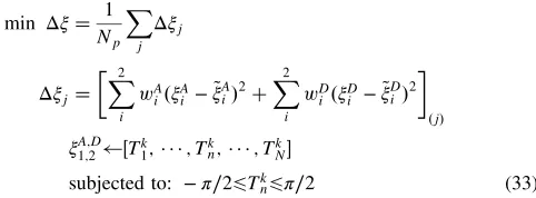
For VAT plates, the fitness function is expressed as a mean value of the least-square distance between the obtained lamination parameters and the target lamination parameters evaluated at a large number of points in the plate [35]. The optimization problem is formulated as
min Δξ 1
Np
X
j Δξj
Δξj
X2
i wA
iξ A i −ξ~
A i
2 X
2
i wD
iξ D i −ξ~
D i
2
j ξA;D
1;2←T
k
1;· · ·; T
k
n;· · ·; TkN subjected to: −π∕2⩽Tk
n⩽π∕2 (33)
whereTk
nis the fiber angle at the control point for thekth ply, andwAi andwD
i are the weights to distinguish the relative importance between
ξA
1;2and ξD1;2. The total number of grid pointsNpis chosen to be 1000∼2000in total for a two-dimensional variation. Based on our trial-and-error experiences, the population size was set to be at least 20∼30times the number of design variables, whereas the number of generations is usually set to50∼100, depending on the population size. The crossover and mutation probabilities were chosen to be 0.7 and 0.04. As the second-level optimization procedure is rapid, several trials can be carried out with different initial values, generation sizes, and population sizes to ensure that repeatable results are achieved.
As the objective function in Eq. (33) is not buckling-load-oriented (least-square-distance based), the optimization process may result in a local optimum with respect to the buckling load. The buckling load of the optimized VAT fiber angles from Eq. (33) is slightly lower (around 10∼15%) than the target result given by the optimal lamination parameters. The fiber angles at the control points can be
further optimized by adding the buckling load as a sensitivity-based constraint [43,44]. A small number of iterations (less than 10) are able to yield a good VAT design that matches well with the global optimal solution from the first-level optimization process. Once a smooth distribution of nonlinear fiber-orientation angles is determined, it is straightforward to construct the manufacturable fiber (tow) tra-jectories. In future work, manufacturing and other design constraints will be considered in the second-level optimization process to generate manufacturable fiber courses.
V. Results and Discussion
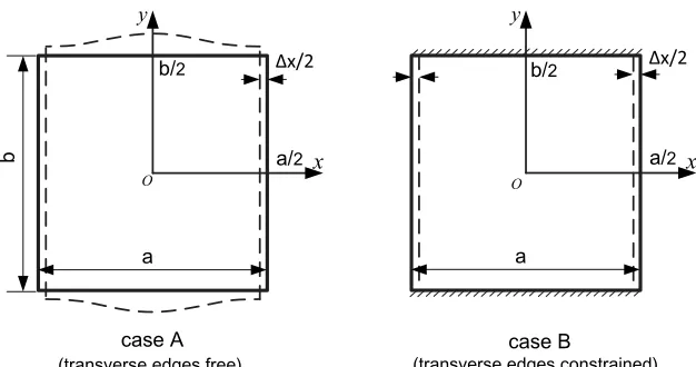
This section presents the numerical results of the proposed two-level optimization strategy to design VAT plates for maximum buckling load. For a clear comparison, the material properties and the geometry of VAT plates in the present study are the same as previous works [1,2,5]. The lamina properties for the T300/5208 graphite– epoxy composite are E11181 GPa, E2210.273 GPa, G12
7.1705 GPa, andν120.28[2]. The tow thickness is 0.127 mm. The thickness variation of a VAT plate due to the manufacture process is not considered in the present study, and the ply thickness is assumed to be constant. Two different in-plane boundary conditions for VAT plates under uniaxial displacement compression are studied, as il-lustrated in Fig. 4. The plate is subjected to uniform displacement compression (x a∕2: u∓Δx∕2) and, in case A, the transverse edges are free to move (stress free,Ny00); in case B, the
transverse edges are constrained (v0).
To give a direct layup comparison, the buckling load of a VAT plate is normalized with respect to that of a homogeneous quasi-isotropic laminate [3]:
Kx
N^crxvat
Ncr
xiso
(34)
whereN^crxvatis the average compressive load:
N^cr
xvat 1 b
Zb 2
−b 2
Nxydy (35)
and Ncr
xiso is the critical buckling load of the quasi-isotropic laminate. The equivalent Young’s modulusEiso, Poisson’s ratioνiso,
[image:8.585.126.458.48.202.2] [image:8.585.136.449.579.744.2]and bending stiffnessDisoof the quasi-isotropic laminate are given by
[35,45]
Diso
Eisoh3
121−ν2 iso
; νisoU4
U1
; EisoU11−ν2iso (36)
A. Optimal Lamination Parameters (First Level) 1. Square VAT Plates
The two-level buckling optimization strategy presented is first applied to determine the optimal design for maximizing buckling performance of square VAT plates with all edges simply supported. The length and width of plate area0.254 mandb0.254 m, respectively. This problem was also studied by Ijsselmuiden et al. [5] using a finite element-based design scheme. This section dem-onstrates the advantage of using B-splines to represent the variation of lamination parameters.
To examine the rate of convergence, the number of control points (in Fig. 5) is gradually increased from 5 to 11 along each direction. In
Fig. 3 Two illustrations for the nonlinear variation of fiber-orientation angles over the VAT plate domain. The fiber angles are parabolically varying along eitherxdirection (left) or both axes directions (right).
Fig. 4 Two cases of in-plane boundary conditions.
each optimization run, all the control points are uniformly distributed across the plate domain and uniform quadratic B-spline basis functions are used for constructing the variation of lamination parameters. The initial values of all lamination parameters at each control point are chosen to be zero, which corresponds to a quasi-isotropic layup. This also enables designers to compare the improvement in VAT laminate performance over a quasi-isotropic layup. Due to the symmetry of the buckling problem in terms of boundary conditions, geometry, and loadings, the lamination pa-rameter distribution is designed to be doubly symmetric; that is,
ξA;D
1;2x; y ξ
A;D
1;2jxj;jyj. The control points for the B-splines that
are used to define the lamination parameters distribution are shown in Fig. 1. The corresponding knot vectors are also chosen to be uniform as
Ξ5 0;0;0;1∕3;2∕3;1;1;1;
Ξ7 0;0;0;1∕5;2∕5;3∕5;4∕5;1;1;1;
Ξ9 0;0;0;1∕7;2∕7;3∕7;4∕7;5∕7;6∕7;1;1;1;
Ξ11 0;0;0;1∕9;2∕9;3∕9;4∕9;5∕9;6∕9;7∕9;8∕91;1;1 (37)
Table 1 lists the obtained maximum normalized buckling loadK cr
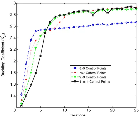
using different numbers of control points, for both case A and case B. Besides the quasi-isotropic laminate, two layups 45 and 36∕∓36∕ 24∕∓24∕04ASwith maximum buckling loads among the constant-stiffness laminates (for each case) are also presented for comparison. The optimal normalized buckling loads of VAT plates are 2.9 and 2.0 for case A and case B, respectively, which indicates more than a 125 and 60% improvement of buckling resistance over the best layup of constant-stiffness laminates. It was observed that, for both cases,7×7control points for the B-splines to define the stiffness variation are sufficient to yield converged buckling opti-mization results. Figure 5 shows the convergence trends of the first-level optimization process for the boundary conditions of case A, using different numbers (5×5,7×7,9×9, and11×11) of control points to construct the lamination parameter distributions. Cor-respondingly, the total number of design variables are 100, 196, 324, and 484. The computational expense for solving the modeling and optimization problem is only slightly increased with using more number of control points. Since the modeling (normally the most time-consuming part) is completely given by analytical formulations, the gradient-based routine only need spend few more internal iterations to complete the first-level optimization process.
All the control-point distributions exhibit rapid convergence within a few iterations (around 10). It is observed that, with an increase of the number of control points, a higher optimal buckling load is obtained. The curves for the7×7,9×9, and11×11control points are nearly coincident when the optimization process con-verges. This also shows that the full design space can be achieved approximately by increasing the number of control points. The optimal variations (7×7control points) of the four lamination pa-rameters are plotted in Fig. 6, for both cases. The contour plots of the
lamination parameters in Fig. 6 exhibit smoothness without notable discontinuity and match well with the results obtained by Ijsselmuiden et al. [5]. However, in the present approach, the number of design variables (196) for achieving convergent optimal results is much less than that (1764) of the finite element ap-proach [5].
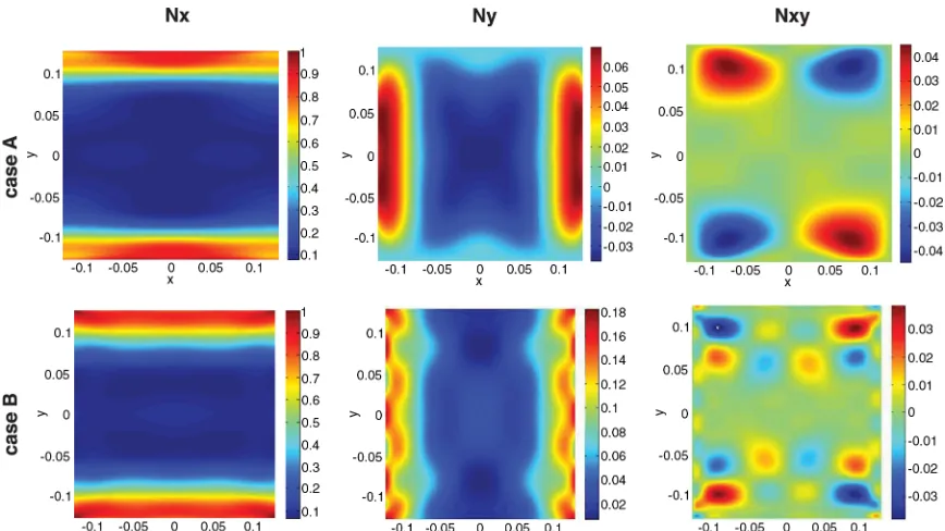
Figure 7 illustrates the in-plane stress distributions (Nx,Ny,Nxy) of the VAT plate with optimal lamination parameter distribution for the maximum buckling load (both case A and case B). It demonstrates that the load redistribution (toward the supported edges) induced by variable stiffness is the main contributing factor to improve the buckling resistance of VAT laminates. It is also interesting to note that a VAT plate subjected to uniaxial compression gives rise to a small amount of internal shear stressesNxydue to the variable stiffness.
[image:9.585.306.544.45.244.2]Representing the lamination parameters distribution in the form of B-splines (or NURBS) exhibits many advantages for the optimal design of VAT laminates. Usage of the B-splines allows the dis-cretization scheme for the stiffness variation to be control-points based and independent of the modeling approach. In a finite element-based design approach [5], the design variables (lamination parameters) are associated with all elements (or nodes); therefore, the design flexibility is fixed to be the same as the degree of freedom of the finite element model. In addition, the number of design variables in a B-spline approach is much less than the finite element method. A smaller number of design variables not only simplifies the design process but also significantly reduces the computational cost for the sensitivities, which is the most time-consuming part in a gradient-based optimization process. Last, the finite element method requires
Table 1 First-level optimization results for the maximum buckling load Kcrx of square VAT plates using different numbers of control points to
construct the lamination parameter distributiona
Case A Case B
Layups K
cr Increase, % Kcr Increase, %
QI 1 — — 1 — —
CS: 45(ξD
1;2 0;−1) 1.29 — — 0.93 — —
CS: 36∕∓36∕ 24∕∓24∕04AS — — — — 1.27 — — (ξA;D1;2 0.64;0;0.4;−0.6) — — — — — —
VAT:5×5 2.66 106.2 1.88 48.0
VAT:7×7 2.89 124.0 1.96 54.3
VAT:9×9 2.92 126.4 2.02 59.0
VAT:11×11 2.92 126.4 2.04 60.6
aQI denotes quasi-isotropic laminate, and CS denotes constant-stiffness laminates.
0 5 10 15 20 25
1.4 1.6 1.8 2 2.2 2.4 2.6 2.8 3
Iterations
Buckling Coefficient (K
*)cr
5×5 Control Points 7×7 Control Points 9×9 Control Points 11×11 Control Points
Fig. 5 Convergence trends of the first-level optimization process using different numbers of control points for constructing the B-spline form variation of lamination parameters along theyaxis.
[image:9.585.168.417.642.745.2]additional constraints [5,14] for constructing a smooth lamination parameter variation; however, B-splines satisfy this requirement inherently.
2. Long VAT Plates
In this section, the design of infinitely long VAT plates for maximizing buckling performance is presented. The length of a VAT plate was selected to be 20 times its width (a5.08 m, b
0.254 m) to adequately capture the (infinitely) long plate effect. Two different out-of-plane boundary conditions are studied: 1) four edges are all simply supported; and 2) one free edge and the rest are simply supported. As the majority of applied compressive load is re-distributed toward the supported edges, the case of transversely varying lamination parameters is initially considered in the opti-mization. Thus, the four lamination parameters are varied along the y directionξA;D1;2y. For the simply supported boundary conditions, the
stiffness variation is defined symmetrically with respect to thexaxis, as
ξA;D
1;2y ξ
A;D
1;2jyj
However, this symmetric condition is not valid in the design of the free-edge problem. For prismatic stiffness variation, closed-form solutions are available for computing the nonuniform in-plane stress [2,46]:
Nx
A11y−A 2 12y
A22y Δx
a (38)
Using Eq. (38) to model the prebuckling behavior of VAT plates can significantly reduce the computational cost of the buckling analysis and sensitivity evaluation. Figures 8 and 9 show the optimal
Fig. 6 Optimal lamination parameter distribution for a square VAT plate under two different in-plane boundary conditions (case A and case B):7×7 control points.
Fig. 7 In-plane stress distribution of VAT square plates with optimal lamination parameters (case A and case B).
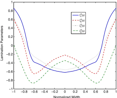
[image:10.585.89.495.44.266.2] [image:10.585.76.510.498.742.2]variations of the four lamination parameters for the long VAT plates under both boundary conditions, in which seven (symmetric) and nine (unsymmetric) control points are used for achieving convergent results, respectively. For the case of simply supported boundary
conditions, the maximum buckling coefficient is 2.61. For the free-edge problem, the maximum buckling coefficient is 4.12. Both of the results are slightly larger than the results obtained from a direct search using the genetic algorithm [3]. Nevertheless, no further improve-ment of buckling load was observed when the lamination parameters (stiffness) are allowed to vary along both axes for the long VAT plate.
B. Optimal VAT Layups (Second Level)
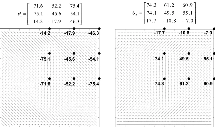
[image:11.585.41.284.46.249.2]Realistic variation of fiber-orientation angles (or the tow trajectories) for the VAT lamination layups are now retrieved from the optimal lamination parameters obtained in the previous section. As previously mentioned, the stacking sequence is fixed to be a 16-layer unsymmetric, specially orthotropic laminate with two VAT design layers. In the optimization process, in each VAT design layer, the number of control points for defining the NLV of fiber-orientation angles [Eq. (32)] is gradually increased to obtain convergent results. In this section, the second-level optimization is carried out on the square plate (under case A) and the long VAT plate with one free edge. Tables 2 and 3, respectively, present (for each problem) the optimal layups and the corresponding improvements of the buckling loads, which are obtained using two different optimization approaches. One is a direct GA search approach based on the definition of NLV of fiber-orientation angles to parameterize the VAT layups [3], and the other is the two-level optimization strategy presented herein. For a clear comparison, the number of control points along each direction that is used to define the NLV of fiber angles of VAT layups was selected to be the same for both methods. A3×3control-points grid is used in each VAT design layer for the square plate, and five control points along the y axis are used for the long plate with a free edge. The results presented in Tables 2 and 3 show that the determined optimal variation of fiber angles using these two methods are slightly different (in terms of the distribution), but they give nearly identical nor-malized buckling loads. This indicates that many optimal VAT layup configurations exist, which give similar buckling loads. This characteristic could benefit the design of VAT laminates when more (practical) constraints are introduced in the optimization process.
A direct GA search approach requires many (population size×the number of generations) buckling evaluation runs for the design of VAT plates. The computational effort increases considerably when many layers and control points are used. Nevertheless, this issue is avoided in the two-level optimization strategy. For these two problems, less than 10 iterations are required
0 0.25 0.5 0.75 1
−1 −0.5 0 0.5 1
Normalized Width
Lamination Parameters
ξA 1(y) ξA
2(y) ξD
1(y) ξD
2(y)
[image:11.585.41.280.303.498.2]Fig. 9 Optimal variations of the four lamination parametersξA;D1;2 for the maximum buckling load of VAT plates with one free edge, and the others are simply supported.
Table 2 Optimal layups for the maximum buckling load of a square 16-layer specially orthotropic laminates (for case A)
Methods Layups K
cr Increase, %
— — Quasi isotropic 1 — —
— — 45∕∓45AS 1.29 — —
Direct GA
2
47167 49.550 71.551
17 12 45
3 5
θ12
4−−72.565 −−5954 −−59.550.5
14 11.5 6
3 5
θ2
2.71 110
Two level −
2
471.675 52.245.6 75.454.1 14.2 17.9 46.3
3 5
θ12
4 74.174 61.249.5 60.955.1
−17.7 −10.8 −7.0
3 5
θ2
2.73 112
Table 3 Optimal layups for the maximum buckling load of a long SSSF 16-layer specially orthotropic laminates
Methods Layups K
cr Increase, %
— — Quasi isotropic 1 — —
— — 45∕∓45AS 1.70 — —
Direct GA θθ1∶T0..4 −11.5;41.5;56;58;65.5 3.94 131.7 2∶T0..4 4;−20;−58;−67;−70
Two level θ1∶T0..4 17.5;36.5;52.5;56;64 3.95 132.3
θ2∶T0..4 −5;−11;−51;−65;−68
−1 −0.8 −0.6 −0.4 −0.2 0 0.2 0.4 0.6 0.8 1
−1 −0.8 −0.6 −0.4 −0.2 0 0.2 0.4 0.6 0.8 1
Normalized Width
Lamination Parameters
ξA 1(y) ξA
2(y) ξD
1(y) ξD
2(y)
Fig. 8 Optimal variations of the four lamination parametersξA;D1;2 for the maximum buckling load of a VAT long plate (case A).
[image:11.585.307.537.521.603.2] [image:11.585.152.435.645.752.2]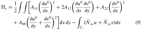

![Dichlorido(1 {(E) [phenyl(pyridin 2 yl κN)methylidene]amino κN}pyrrolidin 2 one κO)copper(II) monohydrate](data:image/gif;base64,R0lGODlhAQABAIAAAP///wAAACH5BAEAAAAALAAAAAABAAEAAAICRAEAOw==)