Filters for M class phasor measurement units

Filters for M class Phasor Measurement Units

Andrew J. Roscoe, Ibrahim. F. Abdulhadi and Graeme

M. Burt

Department of Electronic and Electrical Engineering University of Strathclyde

Glasgow, UK

[email protected]

Abstract— The new standard C37.118.1 lays down strict performance limits for phasor measurement units (PMUs) under steady-state and dynamic conditions. Reference algorithms are also presented for the P (performance) and M (measurement) class PMUs. In this paper, the performance of the Reference M class filter is analysed. Similarly to the Reference P class filter, the M class filter is found to have a relatively poor performance when the power system frequency is off-nominal. A different architecture for an M class Phasor Measurement Unit (PMU) algorithm is presented, and in particular a completely different design of M class filter. This is shown to have much improved rejection of unwanted harmonic and inter-harmonic components. This allows consistent accuracy to be maintained across a ±33% frequency range. ROCOF (Rate of Change of Frequency) errors can be reduced by factors of >100.

Keywords-component; Power system measurements, Fourier transforms, Frequency measurement, Power system state estimation, Phase estimation, Power system parameter estimation, Power system harmonics, Power system stability.

I. INTRODUCTION

A new standard has been published as IEEE C37.118.1 (Measurements)[1] and IEEE C37.118.2 (Data Transfer)[2]. This lays down strict requirements for the required response to dynamic events, and harmonic/inter-harmonic signal content. The required TVE (Total Vector Error) accuracy is still 1%, but the standard also specifies accuracy requirements for frequency and ROCOF (Rate of Change of Frequency) measurements during dynamic conditions. The relationships between measurement windows, reported timestamps, and latency are all described. Furthermore, a Reference algorithm (also called the “Basic synchrophasor estimation” algorithm) is provided, with the implication that it will be compliant if implemented correctly. Testing of PMUs will be possible using new processes produced under the EMRP EURAMET programme [3].

Early analysis of the Basic P class algorithm showed that it can easily meet the required specification for TVE but that meeting frequency and, in particular, ROCOF requirements is much more problematic [4]. Improved versions of the P class PMU were therefore developed [4]. In the case of the P class PMU, the filter is relatively simple and the filter design is

relatively unchanged in the proposed design – it is simply allowed to adapt dynamically in response to the changing power system frequency, so that filter notch frequencies track power system harmonics in real time.

However, in the case of the M class device, the Basic filter is much more complicated, and therefore more difficult to make adaptive. However, the Basic filter makes no attempt to place filter notches at frequencies where harmonics occur (even when f=f0), and this offers a substantial opportunity to improve on its performance.

II. MCLASS FILTER DESIGN

A. The Basic M class filter

The Basic M class filter has a defined pass-band and stop-band, and is of the “brick wall” design (Figure 1). The pass-band has ideally a flat (or at least characterisable) amplitude response across a frequency range defined by the deviation | f-f0| which the algorithm must cope with. This is between 2 Hz for the longest M class filter (Reporting rate FS=10 Hz) and 5 Hz for the shortest (FS=50 Hz), and limits the useful frequency range of the Basic algorithm to these figures. The stop-band should have at least 20dB attenuation, to attenuate both harmonics and inter-harmonics which might appear at mixing frequencies close to 0 Hz if the hardware anti-aliasing filters are not effective.

Figure 1. Basic M class filter frequency response mask [1]

Suitable filter orders, cut-off frequencies, and an equation to calculate filter weights are given in [1] section C.6.

The authors acknowledge the funding and support provided by Rolls-Royce PLC under the UTC (University Technology Centre) programme.

Approximate fitted empirical equations to allow Basic M class filters to be designed for arbitrary sample rates, reporting rates, and nominal frequencies are:

                       S S Basic M _F f F f

L 0 0

_ 5.8943 1.467ln cycles (1)





f    Hz (2)

Where f0 is the nominal frequency, FS is the reporting rate,

L is the filter length in cycles, and fM_Basic is the filter 3dB cutoff frequency.

B. The Proposed M class filter

The Proposed M class filter, by comparison, has the following aims and features:

 A notch is placed at every multiple of the power system frequency, to attenuate harmonics, by using the P class filter as a base.

 The filter is adaptive so these notches move in real time with the system frequency, as described in [4], [5].

 The low-frequency attenuation for close-in out-of-band (OOB) signals is provided by placing 2 further sets of notches at FS/2 (and every multiple of this frequency up to the Nyquist frequency) and at another frequency close by.

 The requirement for ±0.2dB flatness of the filter in the passband is relaxed. This is possible because the quadrature oscillator frequency adapts in real-time to keep the mixing frequency of the wanted fundamental close to 0 Hz at all times [4], [5].

In (1) it can be observed that the Basic M class FIR filter has a time length of approximately 6(f0/FS) fundamental cycles. The Proposed filter actually has a length of 5(f0/FS) fundamental cycles. This is shorter than the Basic filter, but still allows the required performance to be met, while offering slightly reduced response times.

The filter is constructed using cascaded exact-time averaging sections. These allow quick and easy reconfiguration of the notches in real time [6]. Each exact-time averaging section, averaging over a time T, places notches at every multiple of 1/T Hz. The amplitude response of each is given by:              2 2 sin T T G _  (3)

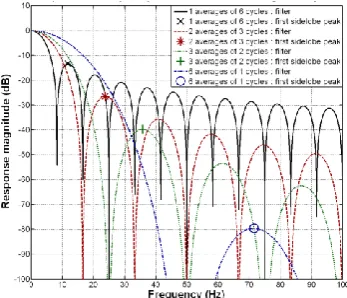
Equation (3) can be solved to show that every averaging section produces a first sidelobe peak at ωT/2=4.493, with a magnitude that is always -13.26dB. Examples of single averaging filter sections can be seen in Figure 2. There is a tradeoff between using small numbers of long filters (which produce notches with lower frequencies and more notches) and

using larger numbers of shorter filters which produce fewer notches but whose responses are convolved together (multiplied in the frequency domain) to provide multiples of the worst-case -13.26dB attenuation across the entire stop-band. For example, Figure 3 shows how 6 cascaded single-cycle filters can produce a higher attenuation of unwanted high-frequency signals than a single 6-cycle average, if attenuation of the lowest frequency signals between 5 and 25 Hz is not of primary importance.

Figure 2. Responses of individual single-stage averaging filters of lengths 1, 2, 3 & 6 cycles (at 50Hz).

Figure 3. Responses of cascaded averaging filters of lengths 1, 2, 3 & 6 cycles (at 50Hz), with total filter lengths of 6 cycles.

When designing the M class filter, a high attenuation is required at a mixing frequency of FS/2 Hz to filter the OOB signals. Therefore, at least one long averaging section of length 2(f0/FS) cycles should be included, putting a notch at FS/2 Hz (and every multiple of FS/2 Hz), and thereby guaranteeing attenuation of 20dB at this frequency. However, this still leaves a substantial filter time period remaining, of (5-2)(f0/FS) cycles, which could be configured in many different ways.

attenuating all harmonics, but having a relatively flat pass-band near 0 Hz (Figure 5).

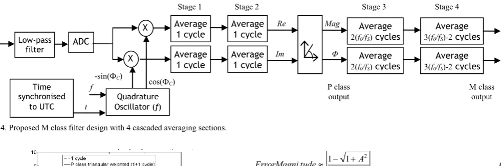
Figure 4. Proposed M class filter design with 4 cascaded averaging sections.

Figure 5. P class filter response

This conversion is done because the response of the long stage 3 and 4 M class filters (using real/imaginary vector signals) is very difficult to characterise, when the mixed signal from the Fourier correlation is not at exactly zero Hz and/or is changing in a “chirp” fashion. This occurs during dynamic frequency events containing ROCOF. By contrast, the short P class filter response is much more easily characterised with a simple sinc() function [4].

Once the conversion to mag/phase is done, the response of the long M class filters is easily defined and characterised. The only problem is that if an interfering signal is large, and not attenuated by the P class filter, then it can impart a gain error onto the measured signal due to the conversion process.

For example, consider a 1pu mixed fundamental at 0 Hz, combined with an interfering signal at amplitude A, which is still present after the P class filter and passes through the real/imag to mag/phase conversion process. Even if the subsequent filtering places a perfect notch at the interfering signal frequency, the measured amplitude of the signal will be:



 





1 _{A A d}

Magnitude (4)



 





1 A A d

tude

ErrorMagni (5)

Equations (4) and (5) are difficult to solve analytically, but can be evaluated numerically. The error magnitude can also be approximated to a good degree of accuracy by the much simpler estimate:

2 1

1 _A2

tude

ErrorMagni    ₍₆₎

The resulting error magnitude against A is shown in Figure 6. This shows that for small signals the resulting error is very small. Most interfering signals are attenuated or notched by the P class filter before the conversion so even large interfering signals usually only result in small values of A. The only exception is during the worst-case M class OOB testing, when a 10% OOB signal at 55 Hz can be applied if FS=10 Hz. This passes through the P class filter with almost zero attenuation, so A is almost 0.1, and an amplitude (TVE) error of almost 0.3% will result, in addition to errors due to finite stage 3 and stage 4 attenuation .

Figure 6. Amplitude error due to the real/imag to mag/phase conversion

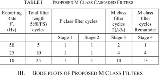
The filter length of the initial P class section is 2 fundamental cycles. This leaves a total time length of 5(f0/FS)-2 fundamental cycles remaining for stage 3 and 4 filters. This is followed by the filter which puts a notch at exactly FS/2 Hz. This leaves a time of 3(f0/FS)-2 fundamental cycles remaining. This, in theory, could be used to provide a further 3(f0/FS)-2 individual cascaded averaging filters of length 1 cycle each. However, for the lowest reporting rate of FS=10 Hz this could result in up to an additional 13 cascaded average sections with f0=50 Hz. In practice, due to the response times. results show that the M class PMUs with FS=50 Hz can be more useful than those with FS=10 Hz. For an FS=50 Hz reporting rate, the remaining averaging time is only 3(f0/FS)-2 = 1 cycle and this cannot usefully be split into smaller sections. Therefore, the final 4th stage filter consists of a single average of length 3(f0/FS)-2 cycles.

To illustrate the filter designs, TABLE I and Figure 4 show how the 4 filter stages are cascaded to make up the entire filter.

Low-pass

filter ADC

X Average

1 cycle

Quadrature Oscillator (f)

Re Im Time synchronised to UTC f t X

-sin(ФC) _cos(Ф C) Average 1 cycle Average 1 cycle Average 1 cycle Average

2(f0/fS) cycles

Average

3(f0/fS)-2 cycles

Average

2(f0/fS) cycles

Average

3(f0/fS)-2 cycles Mag

Φ

Stage 1 Stage 2 Stage 3 Stage 4

P class output

TABLEI PROPOSED MCLASS CASCADED FILTERS

Reporting Rate

FS

(Hz)

Total filter length 5(f0/FS)

cycles

P class filter cycles

M class filter cycles 2(f0/fS)

M class filter cycles Remainder Stage 1 Stage 2 Stage 3 Stage 4

50 5 1 1 2 1

25 10 1 1 4 4

10 25 1 1 10 13

III. BODE PLOTS OF PROPOSED MCLASS FILTERS

This section presents bode plots of the Basic and Proposed filters for a single case of FS=50 Hz, with f0=50 Hz and the sampling frequency FADC=10 kHz. Figure 7 shows that the filter weight distributions are not markedly different. The Proposed design does not need to ever work out the actual filter weights since the filter is implemented as cascaded averages. Negative weights are also never required in the proposed design since the filter does not have such strict requirements for flatness or “brick wall” design.

Figure 7. Filter weights for Basic and Proposed designs, FS=50 Hz.

Figure 8 shows the attenuation of the Basic and Proposed filters around the required cutoff frequency, and through the 1st _{harmonic. The Proposed design has a slightly poorer}

attenuation in the region between FS/2 and about 45 Hz, but otherwise a better performance, particularly at 50 Hz where DC offset and 2nd _{harmonic signal components will mix to.}

Figure 8 also shows how the attenuation of the dominant signal is much lower, given by the P class filter response (Figure 5), due to the conversion from real/imag to mag/phase before stage 3 and 4 averaging.

Figure 9 shows the important region around 100Hz, where the unwanted component of the fundamental will mix to. The Basic response is around -80dB at this point, which is significant but not as good as the deep notch provided by the Proposed filter.

Figure 10 shows the wideband response of higher frequency harmonics, interharmonics and noise, where the Proposed filter shows much deeper attenuation than the Basic filter.

Figure 8. Response at low frequencies for Basic and Proposed designs,

FS=50 Hz.

Figure 9. Response at the important 2nd _{harmonic for Basic and Proposed}

designs, FS=50 Hz.

Figure 10. Wideband response to high frequency harmonics and interference for Basic and Proposed designs, FS=50 Hz.

IV. TIME DOMAIN PERFORMANCE ASSESSMENT

A. Test signal

To test the Proposed design against the Basic algorithms, a 35-second test scenario is generated. This contains OOB, harmonic and ROCOF conditions for the PMU algorithms to contend with. The test uses signal conditions based on those in C37.118.1. The scenario is described in TABLE II.

The sample rate used for the PMU algorithms is 10 kHz. This is achievable in real-time for the Proposed algorithms, and is also not dissimilar to 8kHz rates available on commercial devices [7]. A first-order 2.5kHz low-pass filter is modelled and calibrated for. A 14-bit ADC (analogue to digital converter) is also modelled [8], [5], which samples the signal over a ±2pu range so there are 13 effectively useful bits for a ±1pu nominal voltage signal.

To enable the easiest comparison of the results, between the different PMU designs, only the measurement errors (compared to the known generated signal) are presented in the figures below. Since the raw error plots can appear quite noisy, the errors are presented as unsigned magnitudes. The errors within ±½ of the allowed response times from each sudden signal change are also ignored (set to zero). The error datapoints are smoothed by taking the maximum of the nearest 11 errors in time (5 points either side), and assigning this maximum error to each report datapoint.

TABLEII TEST SCENARIO

Time (s) Signal

From To

-3 0 50 Hz balanced sinusoids, no harmonics (settling) 0 10 Out of band signals (balanced), 10% amplitude, at 55,

65, 75, 85 & 95 Hz (2 seconds each) then remove 10 20 Out of band signals (balanced), 10% amplitude, at

3580, 3590, 3600, 3610 & 3620 Hz (2 seconds each) then remove

20 22.5 50 Hz balanced sinusoids, no harmonics 22.5 25 Add 10% 5th _{(balanced) then remove}

25 28 Add unbalance of 2% plus harmonics 2-40 at amplitudes allowed by Table 2 of EN 50160[9], scaled by 0.7016 to give an overall THD of 8%, with phases correlated for odd harmonics and random for even harmonics. Retain these additions for the remainder of the scenario.

28 32.7 Frequency ramp from 49.5-47 Hz in a non-linear fashion, starting at -1 Hz/s

32.7 35 Constant frequency of 47Hz

B. Results

1) Reporting rate 50 Hz

When FS=50 Hz the PMU is not required to meet the specifications for OOB signals at 55 and 65 Hz (between t=0 and 4s). Figure 11 shows that the 1% TVE specification is indeed not met during this time, by either the Basic of Proposed PMU designs. However, both PMU designs are TVE compliant for the remainder of the scenario.

Frequency measurement accuracy for both PMU designs is compliant across the scenario, except for the time during the 85 Hz OOB signal application, when the Proposed design is not compliant to the ±0.01Hz level [1], whereas the Basic design is (just). This makes sense given the relative filter performances at 35Hz in Figure 8, but also implies that the 20dB mask in Figure 1 is not sufficient to meet the frequency accuracy specifications. Across the remainder of the test, the Proposed design offers a factor of 10 to 100 reduction in frequency error.

Figure 11. TVE for Basic and Proposed designs, FS=50 Hz.

Figure 12. Frequency error for Basic and Proposed designs, FS=50 Hz.

Figure 13. ROCOF error for Basic and Proposed designs, FS=50 Hz.

2) Reporting rate 10 Hz

When FS=10 Hz the PMU has much longer stage 3 & 4 filters. This enables filtering of all OOB signals to within 5 Hz of the fundamental. By contrast to the FS=50 Hz results, the following points are notable:

Firstly, both PMUs are TVE compliant for all OOB signal applications in this test, although note that in this scenario the mixing frequencies exactly match the stage 3 filter notches which is not representative of all cases. Secondly, the Basic PMU has difficulty maintaining TVE accuracy when frequency moves below 48 Hz (Figure 14), since the filter bandwidth is only 2 Hz and accurate amplitude calibration is awkward. Thirdly the Proposed design shows a very low frequency and ROCOF measurement error during the OOB testing (Figure 15 & Figure 16) because the mixing frequencies exactly match the stage 3 filter notches (in this exact case). However, the TVE for the Proposed design is not zero during OOB testing, due to the gain error introduced by (6).

Figure 14. TVE for Basic and Proposed designs, FS=10 Hz.

Figure 15. Frequency error for Basic and Proposed designs, FS=10 Hz.

(Proposed trace goes below the x axis for much of the plot).

Figure 16. ROCOF error for Basic and Proposed designs, FS=10 Hz.

Finally, it is notable that apart from the closest OOB frequencies, the errors from the FS=10 Hz PMU are not usefully smaller than those of the FS=50 Hz PMU. In fact, when ROCOF events occur, the FS=50 Hz device produces lower TVE, Frequency and ROCOF errors than the FS=10 Hz device, and with a shorter response time. This is due to the complicated response of longer PMU filters to a chirp signal.

V. CONCLUSIONS

A new filter is proposed for M class PMU devices. This creates a Fourier-based measurement which is different to a windowed Hanning, Hamming or Flat-top transformation. The filter design is optimised to reject harmonic frequencies and required OOB (out of band) inter-harmonics within PMUs, in conjunction with an adaptive frequency tracking quadrature oscillator. The filter design is tailored so that the entire Fourier correlation and filter can be adapted, reconfigured and executed in real-time at the full ADC sample rate to 10 kHz.

The filter uses a hybrid design. This uses an existing P class filter, followed by a conversion from a real/imaginary pair to a magnitude/phase pair, followed by two longer cascaded filter sections which filter the low-frequency OOB signals.

Due to the improved performance of the filter, in particular the adaptive tracking of the filter notches to the power system harmonics, the measurement error of ROCOF (Rate of Change of Frequency) can be reduced by a factor of more than 100 (40dB) relative to the Reference/Basic PMU design, particularly during times of harmonic contamination and ROCOF events. It is also noted that, apart from the closest OOB signal filtering requirements, the FS=50 Hz device produces similar or lower TVE, Frequency and ROCOF errors than the FS=10 Hz device, with a shorter response time.

Finally it appears that some of the Frequency and ROCOF accuracy requirements of [1] are not achievable using either the Reference PMU or the filter mask of Figure 1 during OOB testing.

REFERENCES

[1] IEEE, "IEEE Standard for Synchrophasor Measurements for Power Systems," C37.118.1-2011, 2011.

[2] IEEE, "IEEE Standard for Synchrophasor Data Transfer for Power Systems," C37.118.2-2011, 2011.

[4] A. J. Roscoe, I. F. Abdulhadi, and G. M. Burt, "P-Class Phasor Measurement Unit Algorithms Using Adaptive Filtering to Enhance Accuracy at Off-Nominal Frequencies," in IEEE SMFG 2011 Smart Measurements For Future Grids, Bologna, Italy, 2011.

[5] Arbiter Systems, "Model 1133A Phasor Measurement Specifications," 2012 Available:

http://www.arbiter.com/files/product-attachments/1133_phasor_measurement_specifications.pdf, accessed April 2012.

[6] A. J. Roscoe, R. Carter, A. Cruden, and G. M. Burt, "Fast-Responding Measurements of Power System Harmonics using Discrete and Fast

Fourier Transforms with Low Spectral Leakage," in 1st IET Renewable Power Generation Conference, Edinburgh, Scotland, 2011.

[7] Schweitzer Engineering Laboratories (SEL), "SEL-451-5 Protection, Automation, and Bay Control System," 2012 Available:

http://www.selinc.com/, accessed April 2012.

[8] M. Lixia, C. Muscas, and S. Sulis, "On the accuracy specifications of Phasor Measurement Units," 2010 IEEE International Instrumentation and Measurement Technology Conference I2mtc 2010, Proceedings,

2010.