Optimal Placement of Phasor Measurement Units by Genetic Algorithm

(1)

doi: 10.11648/j.ijepe.20130201.12

Optimal placement of phasor measurement units by

genetic algorithm

Allagui B., Marouani I., Hadj Abdallah H.

ENIS, Dép. Génie Electrique

Email address:

[email protected] (A. B.), [email protected] (M. I.), [email protected] (H. Abdallah H.)

To cite this article:

Allagui B., Marouani I., Hadj Abdallah H.. Optimal Placement of Phasor Measurement Units by Genetic Algorithm. International Jour-nal of Energy and Power Engineering. Vol. 2, No. 1, 2013, pp. 12-17. doi: 10.11648/j.ijepe.20130201.12

Abstract:

Monitoring and supervision of power systems are provided by the control center, whose role is the design, coordination and network management. This paper presents a control technique based on the implantation of measurement units at the network buses. This technique should meet two requirements: ensure the complete system observability and find the optimal locations of PMUs with the minimum cost. The problem was formulated as a mono-objective optimization problem and its resolution was made by implementing a genetic algorithm (GA). The proposed method is tested on three tests networks and the results are compared with other resolution techniques. The simulation results ensure the complete system observability and validate the presented technique.

Keywords:

PMU, Optimal Placement, Complete System Observability, Genetic Algorithm

1. Introduction

The electrical power networks are continuously pushed to function at the limit of their stability. This is due to several economic, ecological, and technical constraints. In addition to these constraints, the opening of new markets increases the power consumption as well as the complexity of interconnections between the electrical power networks, thus, creating an important energy exchanges on the net-work gridlines. The exchanges on the netnet-work at the mo-ment of an imbalance are visible by the oscillation of the power transiting on the network gridlines. This oscillation limits energy production of the machines and surpasses the generators’ capacity. This fact highlights the importance of the monitoring of electrical power networks using adequate and modern methods.

Currently, many devices are developed to provide near instantaneous measurements (phase, current, and voltage). Such devices are called Phasor Measurement Units (PMU), [1-2]. This technology can provide a precise description of the real time state of the network operating conditions; thus, providing its total observability [3-4], correcting the errors related to mathematical representation, and improving the estimation of these conditions. The bus of the electrical power networks guarantees the visualization of the system which assists the operator to implement an automatic plan to maintain the stability of the network. That also reduces

the number of monitoring personnel, as well as the risks of damage to the equipment in case of a sudden blackout.

The installation of PMUs in the electrical supply net-works resulted in the development of several algorithms to determine the optimal placements of these devices. Such algorithms must be cost effective therefore using the mini-mum of these devices to ensure the total observability of the entire network.

The objective of this work consists in developing a MATLAB program that is based on the genetic algorithms to find the optimal placement of PMUs. The genetic algo-rithm method was tested on three network-tests, and the results were compared with other algorithms. The results of simulation prove that an optimal placement of PMUs en-sures a total observability of the network and thus confirm-ing the efficacy of genetic algorithm [5].

Reference [6] presents a detailed analysis of the required synchronization accuracy of several phasor measurement applications.

(2)

for real time phasor data transmission [7].

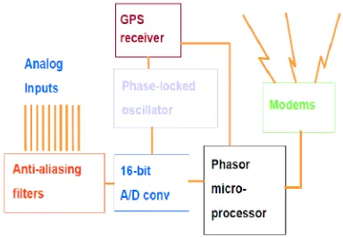
Figure 1. Phasor Measurement Unit Hardware Block Diagram.

2. Terms and Concepts of Observability

The definition of certain terminologies is necessary to better understand Observability [8]:

A directly observable node is a node where a PMU is placed to measure the amplitude and phase of the voltage.

A node, without PMU, is calculable provided that there is a connection in at least one PMU.

A node is unobservable when one or more variables needed to determine its condition is missing.

The complete observability refers to a system where all nodes are directly observable or calculable.

The incomplete observability refers to a system where some nodes are not observable.

To assure the total observability of the network certain rules must be respected:

All nodes neighboring a node with a PMU are observa-ble (figure2).

Figure 2. Example of the first rule of observability.

If a node with zero injection (node which does not inject any power into the network) is observable and all neigh-boring nodes are observable except one, this last one be-comes observable (figure 3).

Figure 3. Example of the second rule of observability.

If all neighboring nodes to a zero injection node are ob-servable, then this node is also observable (figure4).

Figure 4. Example of the third rule of observability.

Given the high cost of phase measurement unit, the number of PMUs must be minimized. The goal is to deter-mine the optimal location of PMUs ensuring total observa-bility.

3. Problem Formulation

3.1. Cost Function Formulation

The installation minimal cost F (X) [5], is directly linked to a minimal number of Placing PMUs.

The minimization function may take the following form:

F (X) = Min ∑ Ci * xi (1)

With:

Ci: The cost to install a PMU at the ith bus.

: 1 ₀ (2)

(3)

The definition of observability constraints is studied in two cases as follows:

a. Case of a network with no zero injection nodes Let the function Cost = F (X) [5] to minimize under the constraints g (X) as g (X) ≥ I

Where g(X)=A×X is a series of equations representing the system topology. The matrix A between two nodes k and m is defined as follows:

,

1 1 ! ! 0 "

(3)

The vector I is the unit vector of dimension (N × 1) with N the total number of network node.

b. Case of a network with zero injection nodes

The study of this case is done using the matrix develop-ment method.

Solving the equation A × X ≥ I will undergo some trans-formations to get a faster and easier resolution by having the form :

A1 × X ≥ b then A1×X = Tcont×P×A×X ≥ b (4)

With:

Tcont : constraint matrix related to nodes with no zero in-jection, it is as follows:

#$%&' ()*)₀ _#0_&+, (5)

Tinj : constraint matrix related to the nodes with zero in-jection, of dimension [x × y] with x represents the number of the nodes with zero injection and y represents the num-ber of the nodes connected to zero injection nodes + 1 (without repetation of the nodes which have more than one connection).

[ ]

1

1,

1, ,

,

1,

1, ,

0,

=

= …





=



= …





If k m ,i

m

A i j

If k et m are connected , j

k

Otherwise

(6)

m: numbers of nodes with zero injection.

k: numbers of nodes connected to the zero injection nodes.

I: identity matrix [M×M], where M represents the num-ber of nodes not connected to the zero injection nodes.

P: Is a permutation matrix between old and new con-straints with a dimension of [N×N], where N represents the total number of nodes in the system; ie it is the identity matrix except with disordered rows, we put the rows of the nodes with no connection to any zero injection node at the beginning, and keep the organization of the columns.

, 1 _{0 "} (7)

b : vector of numbers of PMUs needed to ensure the ob-servability of system, size (a×1) with a is the number of

constraints.

- 1 . / ! ! !

0 "

(8)

For the case of a network with a no zero injection node, the limit number of PMUs needed to assure the observa-bility of this node is equal to 1.

In the case of a network with a zero injection node the limit number of PMUs needed to assure the observability of this node is directly related to the number of nodes to which it is connected.

For example, for a node K, with zero injection, related to the nodes r, t and q, its constraint of observability is: g ≥ 3, since it is related to three nodes (r, t, q).

The formulated problem is a mono-objective optmisation problem with constraints and that could be solved using the genetic algorithms.

4. Genetic Algorithms

The genetic algorithms are stochastic techniques of op-timization which try to imitate the processes of natural evolution of the species and the genetics. They act on a population of individuals subjected to a Darwinian selec-tion: the individuals, known as parents, best adapted to their environment survive and can reproduce. They are then subjected to mechanisms of recombination similar to those of the genetics. Exchanges of genes between parents results in the creation of new individuals, known as children.

The genetic algorithms basically differ from the other methods in research of the optimum:

They act on a set of configurations (populations) and not a single point.

They use only the values of the function to be optimized, not its derivative or other auxiliary information.

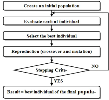
They use probabilistic transition rules (no deterministic). The following functional flow chart illustrates the struc-ture of the genetic algorithm [11].

(4)

The definitions of different steps of the genetic algo-rithm are defined as follows:

Selection: This operator's role is to detect which individ-uals of the current population will be allowed to reproduce ("parents"). Selection is based on the quality of individuals, estimated using a function called "fitness," "evaluation function," or "performance." The methods of selection are: by rank, Steady State, by casino roulette, N / 2 elitism, and tournament.

Evaluation: This step is to calculate (or estimate) the quality of newly created individuals. Here, and only here, that the function to be optimized intervenes. No assump-tions are made about the function itself, except that it must be the basis for selection process.

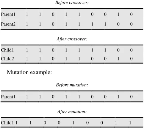
Reproduction: The selected parents are used to generate descendants. The two principal operations are the crossover, which combine genes of 2 parents, and the mutation which consists of a light disturbance of the genome. These opera-tions are applied arbitrarily using two parameters; the probability of crossing and the probability of mutation. These probabilities are important parameters, which consi-derable influence in the quality of final results.

There are several types of crossings and mutations: Crossover : binary crossing, real crossing, arithmetic crossing.

Mutation : binary mutation, real mutation, uniform mu-tation, non uniform mutation.

Crossover example:

Before crossover:

Parent1 1 1 0 1 1 0 0 1 0

Parent2 1 1 0 1 1 1 1 0 0

After crossover:

Child1 1 1 0 1 1 1 1 0 0

Child2 1 1 0 1 1 0 0 1 0

Mutation example:

Before mutation:

Parent1 1 1 0 1 1 0 0 1 0

After mutation:

Child1 1 1 0 0 1 0 0 1 1

Stopping criteria: Stopping the process at the right time is essential from a practical point of view. If there is little or no information about the targeted value of the desired optimum (otherwise stopping happens when this value is achieved by the best individual of the current population), it is crucial to know when to stop the evolution.

In this article, the genetic algorithm with binary coding is employed where each placement of PMU corresponds to binary set with the length equal to the number of node in

the network.

5. Simulation and Results

The algorithm of PMUs optimal placement is tested on three IEEE test networks: IEEE 14 bus, IEEE 30 bus and IEEE 118 bus [8].

5.1. IEEE 14 Bus

The structure of the network IEEE 14 bus is represented by figure 6 where the black spot close to bus 7 indicates a bus with zero injection. The data of the lines and the buses are given by table 1.

Figure 6. Structure of System 14 bus.

Table 1. Data about the IEEE System 14 bus.

System Number of

connections

Number of buses with zero injection

Number of buses with no zero injection

14 bus 20 1 7

5.1.1. Case with No Zero Injection Bus

The results of the simulation are given by the following table:

Table 2. results of network with no zero injection buses.

no zero injection buses

Number of PMUs PMUs placement

Reference solution

[8, 9, 10, 11] 4 2-6-7-9

Solution of

(5)

5.1.2. Case with Zero Injection Buses

Table 3. results of network with zero injection buses.

With zero injection buses

Reference solution

[8, 9, 10, 11] 3 2-6-9

Solution of

genetic algorithm 3 2-6-9

The genetic algorithm produced the same results that are found by the other algorithms published in the IEEE ar-ticles; therefore it is functional for the system 14-bus.

5.2. IEEE 30 Bus

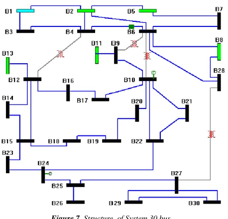
The structure of the network IEEE 30 bus is represented by figure 7. The data of the lines and the buses are given by table 4

System Number

of connections

Number of buses with no zero injection

30 bus 41 5 6-9-11-25-28

5.2.1. Case with No Zero Injection Buses

The results of the simulation are given by the following table5.

Table 5. results of network with no zero injection buses.

Reference solution

[8, 9, 10, 11] 10

2-4-6-9-10-12-15-18-25-27

Solution of

genetic algorithm 10

2-4-6-9-10-12-15-19-25-27

The genetic algorithm produces the same number of PMUs as that of the references, but the localizations of PMUs are not the same.

Table 6. results of network with zero injection buses.

Reference solution

[8, 9, 10, 11] 7

2-4-6-9-10-12-15-18-25-27

Solution of

genetic algorithm 7

2-4-6-9-10-12-15-19-25-27

5.3. IEEE 118 Bus

The structure of the network IEEE 118 bus is represented by figure 8. The data of the lines and the nodes are given by table 7

System Number

of connections

Number of buses with no zero injection

118 nodes 179 10

(6)

5.3.1. Case with No Zero Injection Buses

Table 8. results of network with no zero injection buses 118.

Number

of PMUs PMUs placement

Reference solution [8, 9, 10, 11]

32 2-5-9-11-12-17-21-24-25-28-34-37 -40-45-49-52-56-62-63-68-73- 75-77-80-85-86-90-94-101-105-110-114 Solution 1 of genetic algorithm 32 3-5-9-12-15-17- 21-23-25-28-34- 37-40-45-49-53-56-62-64-69-71- 75-77-80-85-86-90-94-101-105-110-114 Solution 2 of genetic algorithm 32 3-5-9-11-12-17-21-25-29-34-37 -40-45-49-52-56-62-64-69-70-71- 77-80-85-86-90-94-101-105-110-114-118 Solution 3 of genetic algorithm 32 3-5-9-12-15-17-21-23-29-30 -34-37-42-45-49-53-56-62-64-69 -71-75-77-80-85-86-90-94-101-105-110-115

All the solutions are optimal, it is a problem of identifi-cation of the cost it is all.

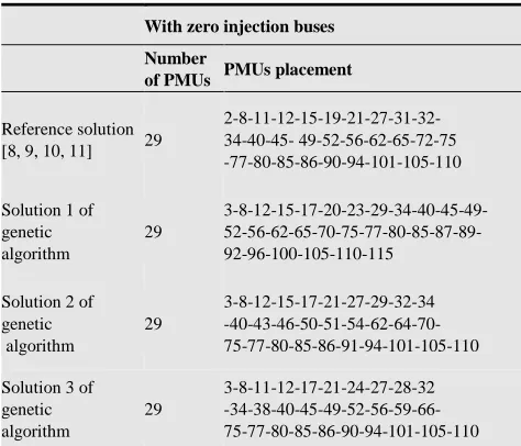
Table 9. results of network with zero injection nodes 118.

Number

of PMUs PMUs placement

Reference solution

[8, 9, 10, 11] 29

2-8-11-12-15-19-21-27-31-32- 34-40-45- 49-52-56-62-65-72-75 -77-80-85-86-90-94-101-105-110

Solution 1 of genetic algorithm 29 3-8-12-15-17-20-23-29-34-40-45-49- 52-56-62-65-70-75-77-80-85-87-89- 92-96-100-105-110-115

Solution 2 of genetic algorithm 29 3-8-12-15-17-21-27-29-32-34 -40-43-46-50-51-54-62-64-70- 75-77-80-85-86-91-94-101-105-110

Solution 3 of genetic algorithm 29 3-8-11-12-17-21-24-27-28-32 -34-38-40-45-49-52-56-59-66- 75-77-80-85-86-90-94-101-105-110

5.4. GA Effects

Table 3, table 6 and the table 9 respectively of 14 bus system, 30 bus system and 118 bus system present the reduced number of PMUs, which allows for a minimization of the cost function with an adjustment in the depths of unobservability of buses.

6. Conclusion

The problem of optimal placement of PMUs (Phasor measurement Units) in an electrical power network is de-fined using certain constraints to guarantee a total observa-bility of the network and to minimize the cost.

It is, thus, a problem of mono-objective optimization where the genetic algorithm is proposed as a method of study. The effectiveness and the flexibility of this algorithm are checked by results of simulation on IEEE test networks.

References

[1] B. Xu and A. Abur, “Optimal placement of phasor mea-surement units for state estimation,” Final Project Report, PSERC, Oct. 2005.

[2] B. Xu and A. Abur, “Observability analysis and measure-ment placemeasure-ment for systems with PMUs,” in proc. IEEE Power Eng. Soc. Power Systems Conf. Expo., Oct. 2004, pp. 943–946.

[3] A. Abur and A. G. Exposito, Power System State Estimation: Theory and Implementation. New York: Mercel Dekker, 2004.

[4] B. Milosevic, M. Begovic, “Nondominated sorting genetic algorithm for optimal phasor measurement placement”, IEEE Transactions on. Power Systems Vol.18, No.1, Feb. 2003, pp. 69–75.

[5] Bei Gou, ’’Generalized Integer Linear Programming Formu-lation for Optimal PMU Placement,’’ IEEE TRANSAC-TIONS ON POWER SYSTEMS, VOL. 23, NO. 3, AU-GUST 2008.

[6] IEEE Working Group H-7, “Synchronized Sampling and Phasor Measurements for Relaying and Control”, IEEE Transactions on Power Delivery, Vol. 9, No.1, January 1994, pp. 442-452.

[7] IEEE Working Group H-8, “IEEE Standard for Synchro-phasors for Power Systems”, IEEE Transactions on Power Delivery, Vol. 13, No. 1, January 1998.

[8] Sanjay Dambhare, ’’Optimal zero Injection Considetrations in PMU Placement : An ILP Approach,’’ 16th PSCC, Glas-gow, Scotland, July 14-18,2008.

[9] J.R.Altman, “A Practical Comprehensive Approach to PMU Placement for Full Observability”, Master of Science In Electrical Engineering, January 28, 2007 Blacksburg, Vir-ginia.

[10] T.A.Baldwin, L. Mili M. B. Boisen, Jr. R. Adapa, “Power system observability with minimal phasor measurement placement”, IEEE Transaction. on Power Systems, Vol. 8, No. 2, May 1993, pp 2381- 2388.