Vibration analysis of a circular plate in interaction with an acoustic cavity leading to extraction of structural modal parameters.
Daniel G Gorman1 Irina Trendafilova1, Anthony J Mulholland2 and Jaromír Horáček3
ABSTRACT
When carrying out vibration health monitoring (VHM) of a structure it is usually assumed that the structure is in the absence of fluid interaction or that any environmental effects which can cause changes in natural frequency either remain constant or are negligible. In certain cases this condition cannot be assumed and therefore it is necessary to extract values of natural frequencies of the structure if it were in the absence of fluid interaction from those values measured. This paper considers the case of a thin circular plate in contact with a fluid cavity giving rise to strong structural/fluid vibration interaction. The paper details the free vibration analysis of the coupled system and through consideration of modal energy, illustrates how the affined modes of vibration of the plate and the fluid can be qualitatively described. The paper then describes a method by which the natural frequencies of the plate in the absence of fluid interaction can be obtained from those of the plate in interaction with the fluid.
Keywords Vibration Health Monitoring, structural/fluid vibration interaction, plates. 1. INTRODUCTION
Vibration Health Monitoring (VHM) of structures is based upon monitoring aspects of the vibration signature of the structure and relating any changes in these to the introduction, or progression, of damage. Damage in a structure, which can be either concentrated (in the form of a crack) or distributed (corrosion, erosion), normally leads to alterations of the stiffness and/or mass, which in turn results in changes in the vibration response of structures. In order to perform successful VHM one has to extract damage sensitive features from the pure structural vibration response (removing the influence of any interacting environment, including the influence of a fluid cavity) [1]. For some structures the natural frequencies can be used as damage sensitive features provided they undergo sufficient changes with the introduction of damage [1-3]. Circular plates are simple structures which lend themselves well to VHM in the sense that their natural frequencies are affected by damage and thus can be used as a basis for damage detection.Another important condition for VHM is that any environmental effects such as temperature stressing and/or structural/fluid interaction remain constant or better still are not present since these effects alone can cause changes to the vibration signature and therefore obscure any changes due to defects in the structure. This paper details the development of a method for extracting the natural frequencies of the plate in the absence of fluid interaction (which can be then used as the basis of VHM) from those values obtained from the plate/fluid cavity coupled system.
The paper commences by presenting a comprehensive analysis of the coupled free vibration of a circular plate in interaction with a fluid filled acoustic cavity. The analysis is based upon a similar analysis of a circular plate in interaction with a fluid cavity [4] which predicted natural frequencies of the coupled system that were in good agreement with values obtained using finite element analysis and experiments. The analysis is based upon the basic equations describing the free vibration of the plate and of the fluid which are then combined using the Galerkin approach. The
1
Department of Mechanical Engineering, James Weir Building, University of Strathclyde, Glasgow G1 1XJ, UK.
2
Department of Mathematics, Livingstone Tower, University of Strathclyde, Glasgow G1 1XJ, UK. 3
analysis proceeds to establish the relative energy between the plate and fluid whilst in interaction and finally describes a method whereby the natural frequencies of the plate in the absence of fluid interaction can be extracted from knowledge of the natural frequencies of the coupled system together with known parameters of the fluid cavity.
2. BASIC ANALYSIS OF THE VIBRATION OF THE COUPLED SYSTEM.
The equation of motion, describing the free small axisymmetric lateral vibration, = (r, t), of a circular disc in interaction with an acoustic cavity, as shown in Figure 1, is
w w
( )
r
,
t
w
Figure 1. Schematic diagram of the plate/fluid interacting system.
D a p t
w D
a h
w d
3
2 2 4
4 +
∂ ∂ −
=
∇ ρ (1) .
where, for axisymetric modes of vibration,
⎟⎟ ⎠ ⎞ ⎜⎜
⎝ ⎛
∂ ∂ + ∂
∂ = ∇
r r r
1 2 2 2
, w =w/a, r = r/a and D=E h3/12(1−μ2);
E is Young’s modulus, μ is Poisson ratio and ρd is the plate density; a and h are the radius and
thickness of the plate, respectively; L is the depth of the cylindrical cavity and p is the acoustic pressure inside.
Now writing w = s s i t
s
e
r ω
ψ χ ( ) 1
∑
∞=
, (2)
where ψs(r) is the natural mode shape of the disc in the absence of fluid interaction and χs is a
constant for that mode, generally referred to as the mode shape coefficient for the mode consisting s nodal circles. In this particular case, for a stressed disc clamped at the periphery, the mode shapes,
) r (
s
ψ , are according to [5]:
) ( )
( ) (
) ( )
( 0 0
0
0 J r I r
J I
r s s
s s
s ξ ξ ξ
ξ
ψ = − + , (3)
where ξs are roots (values of s = 1, 2, 3 etc.) computed from the equation:
(
x,r,t)
p
r
a
L
x
( )
( )
0( )
( )
01
0
1 + =
s s s s I I J J ξ ξ ξ ξ (4)
and I0, I1 and J0, J1 are the Bessel functions (order zero and one).
For a particular value of s, the natural frequency of free undamped vibration, ωs, is then:
4 2 a h D d s
s ξ ρ
ω = (5)
where ξs is a non-dimensional parameter related to the natural frequency ωsof the plate in the absence of fluid interaction. Table 1 below lists values of ξs for the first three ( s = 1,2 and 3) axisymetric modes of a circular plate clamped around the periphery.
[image:3.595.58.483.521.763.2]s ξs 1 3.1962 2 6.3064 3 9.4395
Table 1. Non-dimensional natural frequencies, ξs, for the axisymetric modes of a clamped circular
plate.
For a particular mode of vibration for the disc in the absence of fluid interaction, i.e., substitute equation (2) into equation (1) with p = 0:
[
( )]
( ) 4 r D a hr s d s
s ψ
ρ ω
ψ =
∇ 2 4
(
)
. (6)
Therefore combination of equations (1) and (6) gives:
[
]
ha p e r d t i s s s s ρ ψ χ ωω − ω =
∑
∞ = ) ( 2 2 1. .. (7)
The form of the acoustic pressure, p, acting on the disc will now be established by reference to the acoustic cavity. Consider the acoustic cavity shown in Figure 1, whose velocity potential,
φ = φ(x, r,t), is described by the equation
2 2 2 2 2 2 1 t c a L a r r r ∂ ∂ ⎟ ⎠ ⎞ ⎜ ⎝ ⎛ = ∂ ⎟ ⎠ ⎞ ⎜ ⎝ ⎛ + ∂ ∂ + ∂
∂ φ φ 2 φ 2 φ
, (8) x
∂
and /
,
/ac x = x L
φ c is speed of sound. Now writing
where φ =
t i e r Q x H ω
φ = ( ). ( ) (9) and substituting equation (9) into (8) gives
2 2 1 k Q Q r Q " Q L a ± = ⎥ ⎦ ⎤ ⎢ ⎣ ⎡ + ′ + − ⎜ ⎝
⎛ 2 λ
H " H = ⎟ ⎠ ⎞
, (10)
where
c a
ω
λ = and k is a constant. For the case where the right hand side of equation (10) is
equal to –k2 gives
) r ( Y B~ ) r ( J B ) r (
where α = λ2 −k2 or k = λ2 −α2 and B~=0 since Q(r) must be finite when r →0. At 1
= r
0
= ≡
∂ ∂
r d dQ r
φ
. . (11)
Therefore the condition (11) has roots αq (q = 1, 2, 3 etc.), which satisfy the equation J0′(α )=0.
Similarly cos( ) since 0
0 )
( =
=
= x q
x d dH x
C
H γ ω ,
where q( ) q kq( )
a L a
L ω
ω λ α
γ = 2 − 2 = .
Thus equation (9) becomes:
t i q )
( q q
q
e ) r ( J ) x cos(
B γ ω α ω
φ 0
1
∑ = ∞
= . (12)
At x =1, the axial component of the velocity of the gas and the lateral velocity of the plate must be equal, i.e,
t w x
L c
x ∂
∂ = ∂
∂
=1 φ
for 0≤r ≤1 .
Therefore combining equations (2) and (12) renders
[
B ( )sin( ( ))J0 ( r)]
i (r)L c
s s q
q q
q γ γ α ω χ ψ
ω
ω
∑
∑
∞ = ∞−
1
1 s
q= =
. (13)
Now using the orthogonal properties of the eigenfunction, r J0
( )
αqr , by multiplying both sides of equation (13) by r J0( )
αqr and integrating between 0≤r ≤1 according to reference [6] gives( )
q qs s s qJ k
c L i B
α γ
γ
χ ω
ω
ω 2
0 ) ( ) (
1 ) sin(
2
∑
∞
=
−
= , (14)
q q
where kqs rψs r J0
( )
αqr dr 1) (
∫
=
0
(15)
the value of which can be obtained through standard numerical integration. Now the pressure, p, at the surface of the plate is given by:
1 =
∂t x ∂ −
= f ac
p ρ φ ,
where ρf is the fluid density.
Therefore combining equations (12) and (14) renders:
( )
(
s qs)
q( )
i tf e
r J k aL
p ω ω ω
q q
q
s q γ γ J α
α χ
ρ ω
2 ) ( ) (
0 2
2
∑∑
∞ ∞
− =
0 1 1 tan
= =
. (16)
(
)
(
)
( )
( )
q q q q qs s s q d f s s s s J r J k h L r α γ γ α χ ρ ρ ω ψ χ ωω ω ω
2 0 ) ( ) ( 0 1 1 2 2 2 1 tan 2 ) (
∑∑
∑
∞ = ∞ = ∞ = − = − .Multiplying both sides by rJ0
( )
αqr and integrating between 0≤r ≤1 renders:(
)
0tan 1 ) ( ) ( 2 2 1 = ⎪⎭ ⎪ ⎬ ⎫ ⎪⎩ ⎪ ⎨ ⎧ ⎥ ⎥ ⎦ ⎤ ⎢ ⎢ ⎣ ⎡ − −
∑
∞= γ ω γ ω
ρ ω ω χ q q s qs s s
k , (17)
where plate of mass gas of mass = = h L d f ρ ρ ρ .
Now, since 2 4 4
ha D
d s
s ξ ρ
ω =
a non-dimensional factor η instead of ωcan be introduced and is defined by the relation: 4 4 2 ha D d ρ η
ω = . (18)
Hence equation (17) can be re-written as
(
)
⎪⎭⎪⎬⎫ ⎪⎩ ⎪ ⎨ ⎧ ⎥ ⎥ ⎦ ⎤ ⎢ ⎢ ⎣ ⎡ − −∑
∞ = ( ) ( ) 4 4 1 tan1 η η
γ γ ρ η ξ χ q q s qs s s
k = 0 , (19)
where ( ) 4 2 2 q2
d q c ha D a L α ρ η
γ η = −
.
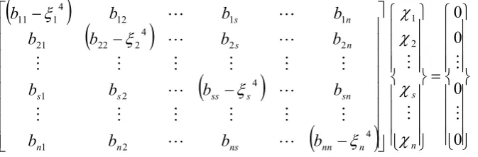
Equation (19) can be represented in matrix form as
(
)
(
)
(
)
(
)
(
)
(
)
(
)
(
)
(
)
(
)
⎥⎥ ⎥ ⎥ ⎥ ⎥ ⎥ ⎥ ⎦ ⎤ ⎢ ⎢ ⎢ ⎢ ⎢ ⎢ ⎢ ⎢ ⎣ ⎡ = ⎥ ⎥ ⎥ ⎥ ⎥ ⎥ ⎥ ⎥ ⎦ ⎤ ⎢ ⎢ ⎢ ⎢ ⎢ ⎢ ⎢ ⎢ ⎣ ⎡ ⎥ ⎥ ⎥ ⎥ ⎥ ⎥ ⎥ ⎥ ⎦ ⎤ ⎢ ⎢ ⎢ ⎢ ⎢ ⎢ ⎢ ⎢ ⎣ ⎡ 0 0 0 0 , , , , , , , , , , 2 1 2 1 2 1 M M M M L M M M L L M M M L L n 2 1 nn n2 n1 2n 22 21 1n 12 11 χ χ χ χ η ξ η ξ η ξ η ξ η ξ η ξ η ξ η ξ η ξ η ξ s n s qs n n a a a a a a a a a a , 0 A( , ) =i.e. ξ ηs s (20)
) , (ξs η
qs
(
)
a ) =
⎪⎭ ⎪⎩ ⎢⎣ ( ) ( ) ⎥⎦
tan η
η γ
γq q s qs ⎪ ⎬ ⎫ ⎪ ⎨ ⎧ ⎥ ⎤ ⎢ ⎡ − − 4
4 η 1 ρ
ξ
k . (21)
Hence values of η can be obtained (iterated upon) which renders the determinant of matrix (20) equal to zero. Consequently for each of these values (roots) of η the corresponding values of mode shape coefficients χ1, χ2, ……… χn, can be obtained. The determinant of this matrix equation is
zero are substituted back into equation (20) to obtain the corresponding values of the mode shape coefficients, s, (normalised to 1 in the first instance and then to the largest value) which describe
which structural modes are present and dominate.
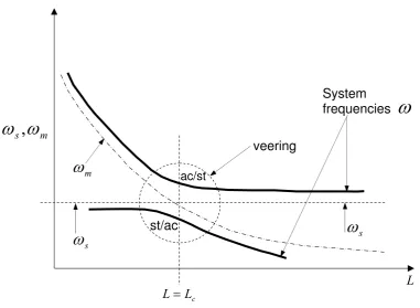
The parameters which will give rise to conditions of strong structural/fluid vibration interaction will now be developed and postulated. Figure 2 shows a plot of a natural frequency, ωs, of the plate in the absence of fluid interaction and the natural frequency, ωm, of the acoustic cavity if the top plate was rigid. Both of these natural frequencies are plotted to a base of the controlling parameters, L; the depth of the cavity. Now, for any value of s, the natural frequency of the plate in the absence of fluid interaction is given by equation (5) and this value is independent of the depth L. A natural frequency of the solid bounded fluid cavity is obtained by now imposing the condition that
∂ ∂ x
c φ
for all r upon equation (12). 0
1 = =
x
L
This results in 2 ; 1,2 etc.
2 2
a2 )
( = − = =
m m c
a L
q m
q
m ω α π
γ ω
Note, in the special case(s) when m=0, this would imply only radial fluid modes with the fluid having zero axial component of velocity, this having no interaction with the transverse (lateral) vibration of the plate. Therefore, for m≥1,
2 1
2 2
⎥ ⎥ ⎦ ⎤ ⎢
⎢ ⎣ ⎡
+ ⎟ ⎠ ⎞ ⎜ ⎝ ⎛
= q
m
L a m a
c π α
ω (22)
and introduces the dimensionless frequency 2
2 2 2
q m
m
L m
c
L α
π π
ω
β = = + (23)
where
a L
L =
This is demonstrated in Figure 2. As L increases all values of ωm decrease and will, for appropriate values of L = Lc correspond to values of ωs of the plate in the absence of fluid
interaction. In such circumstances there is strong structural/fluid vibration interaction characterised by a region of “veering” whence at L = Lc the strongly interacting system will exhibit two natural
Therefore for L = Lc equating equations (5) and (22) gives,
2 1
2 2
2 2
2
) 1 (
12 ⎥⎥⎦
⎤ ⎢
⎢ ⎣ ⎡
+ ⎟⎟ ⎠ ⎞ ⎜⎜ ⎝ ⎛ =
− q
c a
s
L a m a c E
a
h π α
μ ρ ξ
For the purpose of defining an initial state of strong structural/acoustic interaction, the case where q = 1, i.e. q = 0 (zero radial component of fluid velocity) will be applied, whence, for strong
interaction between the plate and the first axial mode of the gas (zero radial), renders the condition.
2 2
2
) 1 ( 12
⎟ ⎠ ⎞ ⎜ ⎝ ⎛ − =
=
h a E
c m a
L
L d
s c
c
μ ρ ξ
π
(24)
and from equation (23) m
c L m
m = π =
ω β
Prior to examining the characteristics of the strongly coupled vibration modes associated with various combinations of s and m, the convergence of the analysis presented will be investigated.
ac/st
veering
st/ac
m
ω
s
ω
ω
sc L L=
L System
frequencies
ω
m s
ω
,
[image:7.595.67.449.138.417.2]ω
For this exercise, and all subsequent results, the following parameters will be adopted; c = 343 m/s
(air), d = 7800 kg/m3, = 0.3, E = 210 GN/m2 and ⎟
⎠ ⎞ ⎜ ⎝ ⎛ h a
= 100.
Convergence
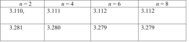
For the convergence analysis consider a plate clamped around its perimeter. Furthermore the dimensions, Lc are selected, in accordance with equation (24), such that strong coupling exists between the first natural frequency of the plate in the absence of fluid interaction (s=1) and the first axial natural frequency (m=1) of the completely bounded cavity. For such a case the value of Lc is 6.7177. Accordingly, Table 2 lists the first two values of η obtained for n (the size of the matrix [A(ξs,η)] of equation (20)) = 2, 4, 6 and 8. Furthermore these same two values of η can be compared with the first natural frequency (s = 1) the plate in the absence of fluid interaction; 1 = 3.1962.
n = 2 n = 4 n = 6 n = 8
3.110, 3.111 3.112 3.112
[image:8.595.38.417.272.358.2]3.281 3.280 3.279 3.279
Table 2 Convergence
From Table 2, it is seen that convergence is extremely fast with respect to n; requiring only n = 6 for a fully converged result to 3 decimal places for these lower modes. Accordingly, forthwith n = 6 will be used throughout. It is noted that the first value of η is lower than 1 and the second one is higher. This is in accordance with the observation shown in Figure 2 atL=Lc.
Energy Analysis.
In this study, since in all cases we are dealing with some degree of structural/fluid vibration interaction, it would be erroneous to describe any mode of vibration as either purely a structural mode or an acoustic (fluid) mode. Rather reference will be made to the modes as either structural/acoustic (st/ac), to denote modes which are predominantly structural with acoustic interference, and likewise acoustic/structural (ac/st) to denote modes which are predominantly acoustic but with structural interference. In an attempt to quantify the degree of coupling and describe whether modes are mainly structural or fluid acoustic, attention will be drawn to the distribution of vibration kinetic energy between the structural and fluid components of the system.
For the plate the maximum kinetic energy of vibration, KEp, is calculated from;
r d r r ha
KE s s
n
s d
p
2
1 1
0 2 4
) ( ⎥
⎦ ⎤ ⎢
⎣ ⎡
=
∫
∑
= ψ χ ω
πρ (25)
and since the eigenvectors, ψs(r), are orthogonal, then,
ps n
s
p KE
KE = ∑
where KEps dha
[
s s r]
2 r dr 10 2
4ω χ ψ ( )
πρ
∫
=
For the fluid the maximum kinetic energy, KEf, is calculated from;
x d r d r V V
L a
KEf f [( r)2 ( x)2] 1
0 1
0
2 +
=πρ
∫∫
(26)where
x L ac V
r c
Vr x
∂ ∂ =
∂ ∂
= φ ; φ
where q q( ) q i t
q
e ) r ( J ) x cos(
B γ ω α ω
φ 0
1
∑ = ∞
=
Therefore xq
n
q x
rq n
q
r V V V
V
∑
∑
= =
= =
1 1
and
Once again, because of orthogonality of the eigenvectors describing φ
x fq n
q r
fq n
q
f KE KE
KE = ∑ + ∑
=
=1 1
where =
∫∫
( )
1
0
2 1
0 2
x d r d r V L a
KErfq ρf π rq
and =
∫∫
( )
1
0
2 1
0 2
x d r d r V L a
KExfq ρf π xq
and both and are now obtained by using equations (12) and (14). Also, the percentage energy associated with and are expressed as,
rq
V Vxq
f
KE KEp
% 100 ) (
% 1 x
p f
x fq n
q x f
KE KE
KE KE
+ ∑
= = for total axial fluid energy
% 100 ) (
% 1 x
p f
r fq n
q r f
KE KE
KE
KE
+ ∑
= = for total radial fluid energy
% 100 ) (
%
and x
p f
p p
KE KE
KE KE
+
= for total plate energy
Also a set of eigenvectors for the plate and fluid is
KE
{
xfn}
xfq x
f x
f x
fq = %KE 1, %KE 2,...,%KE ,...,%KE = vector of axial kinetic energy components of fluid, and,
KEps =
{
%KEp1, %KEp2,−−−%KEps,−−−%KEpn}
= vector of kinetic energy of lateral vibration components of the platewhere %
[
]
x 100%⎪⎭ ⎪ ⎬ ⎫
⎪⎩ ⎪ ⎨ ⎧
+ =
p f
r fq r
fq
KE KE
KE KE
[
]
100%% x
⎪⎭ ⎪ ⎬ ⎫ ⎪⎩
⎪ ⎨ ⎧
+ =
p f
x fq x
fq
KE KE
KE KE
and %
[
]
x 100%⎪⎭ ⎪ ⎬ ⎫ ⎪⎩
⎪ ⎨ ⎧
+ =
p f
ps ps
KE KE
KE KE
Consequently, using the above relative percentage energies, the characteristics of a circular clamped disc in strong interaction with an acoustic cavity as described are investigated. Consider the case where Lc is 6.7177 which, as before, results in a condition of strong coupling between the first mode of the plate in the absence of fluid interaction (s=1), and the first (m=1) axial mode only of
the fluid cavity if the plate is assumed rigid. In all cases the ratio of
h a
= 100 and we will only
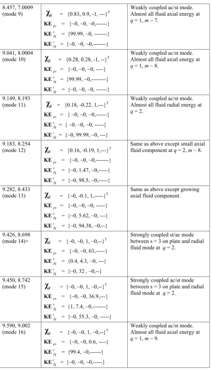
consider roots of the system matrix equation (20-21), η, up to those close to that corresponding to the third of the plate in the absence of fluid interaction, , equal to 9.439. Accordingly Table 3
list the non-dimensional frequency roots,
3
ξ
ηand m, together with the associated vectors;
s
,KE , KE and KE .ps x
fq
η, m Mode Description
3.112, 0.9477
(mode 1) s = { 1, ~0, ~0, ---}T
KEps = { 47.88, ~0, ~0, --- }
KExfq = { 52.03, ~0, ~0, --- }
KErfq = {~0, ~0, --- }
Strongly coupled st/ac or ac/st mode at s = 1, q = 1, m ~ 1.
3.279, 1.0526
(mode 2)+ s = {1, ~0, ~0, --- }T
KEps = { 50.99, ~0, ~0, -- }
KExfq = { 48.91, ~0, ~0,-- }
KErfq = {~0, ~0, ~0, --- }
Coupled ac/st mode at s = 1, q = 1, m ~ 1.
4.524, 2.0033
(mode 3) s = { 1, -0.207, ~0, --- }T
KEps = {0.5, ~0, ~0, --- }
KExfq = { 99.5, ~0, ~0, -- }
KErfq = {~0, ~0, ~0, --- }
Weakly coupled ac/st mode. Almost total fluid axial energy at q = 1, m ~ 2.
5.537, 3.0011
(mode 4) s = { 1, -1, ~0, ~0, -- }T
KEps = { ~0, ~0, ~0, --- }
KExfq = {99.99, ~0, ~0, -- }
KErfq = {~0, ~0, ~0, --- }
Weakly coupled ac/st mode. Almost total fluid axial energy at q = 1, m ~ 3.
6.297, 3.8813
(mode 5)+ s = {~0, 1, ~0, ~0, -- }T
KEps = { ~0, 93.53, ~0, - }
KExfq = { 6.22, ~0, ~0, - }
KErfq = {~0, 1.43, ~0, --- }
Coupled st/ac mode at s = 2, q =1 , m ~ 4.
6.400, 4.0089
(mode 6) s = {~0, 1, ~0,--- }T
KEps = {~0, 6.01, ~0, -- }
KExfq = {93.90, ~0, --- }
KErfq = {~0, ~0, ~0, ---- }
Weakly coupled ac/st mode. Almost total fluid axial energy at q = 1, m ~ 4.
7.148, 5.002
(mode 7) s = {0.54, 1, -0.17,-- }T
KEps = {~0, ~0, ~0, ---- }
KExfq = { 99.9, ~0, ---}
KErfq = { ~0, ~0, ~0, ---- }
Weakly coupled ac/st mode. Almost total fluid axial energy at q = 1, m ~ 5.
7.829, 6.001
(mode 8) s = {0.78, 1, -0.46,-- }T
KEps = {~0, ~0, ~0, ---- }
KExfq = {99.99, ~0, ~0, -- }
KErfq = {~0, ~0, ~0, --- }
Weakly coupled ac/st mode. Almost total fluid axial energy at q = 1, m ~ 6.
8.457, 7.0009
(mode 9) s = {0.83, 0.9, -1, ---}T
KEps = {~0, ~0, ~0,---}
KExfq = {99.99, ~0, ---}
KErfq = {~0, ~0, ~0,---}
Weakly coupled ac/st mode. Almost all fluid axial energy at q = 1, m ~ 7.
9.041, 8.0004
(mode 10) s = {0.28, 0.28, -1, --}T
KEps = {~0, ~0, ~0, ----}
KExfq = {99.99, ~0,---}
KErfq = {~0, ~0, ~0, ---}
Weakly coupled ac/st mode. Almost all fluid axial energy at q = 1, m ~ 8.
9.149, 8.193
(mode 11) s = {0.18, -0.22, 1,---}T
KEps = { ~0, ~0, ~0,---}
KExfq = { ~0, ~0, ~0, ---}
KErfq = {~0, 99.99, ~0, ---}
Weakly coupled ac/st mode. Almost all fluid radial energy at q = 2.
9.183, 8.254
(mode 12) s = {0.16, -0.19, 1,---}T
KEps = {~0, ~0, ~0,---}
KExfq = {~0, 1.47, ~0,---}
KErfq = {~0, 98.5, ~0,---}
Same as above except small axial fluid component at q = 2, m ~ 8.
9.282, 8.433
(mode 13) s = {~0, -0.1, 1,---}T
KEps = {~0, ~0, ~0, ---}
KExfq = {~0, 5.62, ~0, ---}
KErfq = {~0, 94.38, ~0,--}
Same as above except growing axial fluid component.
9.426, 8.698
(mode 14)+ s = {~0, ~0, 1, ~0,--}T
KEps = {~0, ~0, 63,---}
KExfq = {0.4, 4.3, ~0, ---}
KErfq = {~0, 32 , ~0,--}
Strongly coupled st/ac mode between s = 3 on plate and radial fluid mode at q = 2.
9.450, 8.742
(mode 15) s = {~0, ~0, 1, ~0,--}T
KEps = {~0, ~0, 36.9,---}
KExfq = {1, 7.4, ~0,---}
KErfq = {~0, 55.3, ~0, ---}
Strongly coupled ac/st mode between s = 3 on plate and radial fluid mode at q = 2.
9.590, 9.002
(mode 16) s = {~0, ~0, 1, ~0,--}T
KEps = {~0, ~0, 0.6, ----}
KExfq = {99.4, ~0,---}
KErfq = {~0, ~0, ~0,---}
Weakly coupled ac/st mode. Almost all fluid axial energy at q = 1, m ~ 9.
[image:12.595.52.469.35.764.2]
Table 3 lists details of all coupled modes of vibration up to around a frequency corresponding the 3rd natural frequency of the plate in the absence of fluid interaction. From this table it is evident that the modal energy of the subsystems renders an excellent means of describing the degree of coupling and dominance of the structure or fluid. It is also interesting to note that for modes with a strong or moderate structural component, the vector of mode shape coefficients is very well defined. For example for the first two coupled modes (1 and 2) with frequencies around that corresponding to the first
natural frequency of the plate in the absence of fluid interaction, ={1, 0, 0, ---}T and for mode 5 which is once again structurally dominant at a frequency close to that of the second natural frequency of the plate in
the absence of fluid interaction, ={0, 1, 0, 0, 0, ----}T. On the other hand, for modes of a strong acoustic
nature, such as modes 3 and 4 in Table 3, it is observed that the vector indicates significant contributions
from more than one structural mode, e.g., mode 4 where ={1, -1, 0, 0, - }T. This observation of the form of
the vector for modes with a strong or moderate structural energy component will be seen to be important when considering the inverse problem, i.e., the problem of being able to extract the natural frequencies of what the plate would be in the absence of fluid interaction,
s
s
s
s
s
s s
ξ , when one has obtained values of the natural frequencies of the coupled system, η.
3. THE INVERSE EXTRACTION PROBLEM.
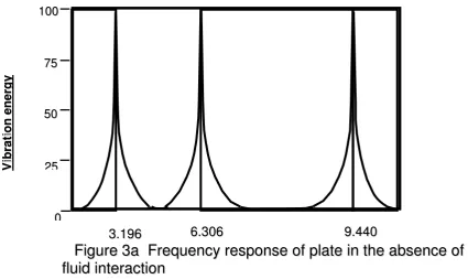
In the foregoing analysis known values of the structural natural frequencies together with the parameters of the fluid cavity were used as the input to computed values of natural frequencies of the structural/fluid coupled system and corresponding vector of structural mode shape coefficients from which the relative levels of vibration kinetic energy were obtained for the structure and the fluid. As was seen from Table 3 a significant difference occurs between the natural frequencies of the coupled system, where there is significant relative vibration energy associated with the structure, and the natural frequencies of the structure in the absence of fluid interaction. (To illustrate this, Figures 3a and 3b show typical plots of vibration energy of the plate in the absence of fluid interaction and the plate in interaction as described (assuming damping to being negligible) up to frequencies around that of the 3rd natural frequency of the plate in the absence of fluid interaction.)
V
Vib br ra at tio on ne en ne er rg gy
y
i
i
3
3..119966
1 10000
7 755
5 500
2 255
0 0
6
6..330066 99..444400
33..111133 66..33 66..44
In such modes however it was observed that the vector of mode shape coefficients, , was well defined with a single unity at the structural mode in question and zeros for all other components. This, as will be seen, is very important with respect to solving the inverse problem.
s
In structural modal analysis and vibration-based damage detection it is the values of the structural natural frequencies alone, , which are of importance. Accordingly, in the case where the structure is in interaction with a fluid cavity (as is the case here), accepting the coupled natural frequencies obtained from experiments upon the coupled system to being sufficiently accurate estimates to the structural natural frequencies, could have grave consequences and give erroneous information. Accordingly, the inverse problem in this case is defined as extracting the structural natural frequencies,
s ξ
s
ξ , from the values of the coupled natural frequencies, η , obtained from experiments and known parameters of the fluid cavity in interaction.
To achieve this, equation (20) can be written in the form;
A(ξs,η) s = (K − K) s =0 (27)
.
.2288 99..4433 99..4455
V
Vi ib br ra at ti io on ne en ne er rg gy
y
1 10000
7 755
5 500
2 255
0 0
94
51 48
6
63
37
where K = (28) ⎥ ⎥ ⎥ ⎥ ⎥ ⎥ ⎥ ⎥ ⎦ ⎤ ⎢ ⎢ ⎢ ⎢ ⎢ ⎢ ⎢ ⎢ ⎣ ⎡ nn n2 n1 2n 22 21 1n 12 11 k k k k k k k k k k qs L M M M L L M M M L L
where kqs rψs r J0
( )
αqr dr 10
) (
∫
= as before, equation (15).
= where
⎥ ⎥ ⎥ ⎥ ⎥ ⎥ ⎥ ⎥ ⎦ ⎤ ⎢ ⎢ ⎢ ⎢ ⎢ ⎢ ⎢ ⎢ ⎣ ⎡ = n s q θ θ θ θ L L M O M M M M L L M M M O M M L L L L 0 0 0 0 0 0 0 0 0 0 0 0 2 1
(
)
⎭⎬ ⎫ ⎩ ⎨ ⎧ −= 4 ( ) ( )
tan
1 η η
γ γ ρ η θ i i i and = ⎥ ⎥ ⎥ ⎥ ⎥ ⎥ ⎥ ⎥ ⎦ ⎤ ⎢ ⎢ ⎢ ⎢ ⎢ ⎢ ⎢ ⎢ ⎣ ⎡ 4 4 4 2 4 1 0 0 0 0 0 0 0 0 0 0 0 0 n s ξ ξ ξ ξ L L M O M M M M L L M M M O M M L L L L
is diagonal matrix containing values of the non-dimensional natural frequencies of the structure alone. Now introducing the matrix B as
B=K−1 K (29) Equation (27) can be written in the form
[
B−]
s =0 (30)Note that the matrix K contains the values of ξs obtained from equations (4) and (15). However it will be assumed that the influence of small changes of ξs(due to the effect of damage to the structure) on the normal eigenfunctions, equation (4), and hence from equation (15) are negligible and the same form of the K matrix, based upon equations (4) and (15), is used irrespective of any changes to
qs k
s
non-dimensional natural frequencies of the structure in the absence of fluid interaction which we aim to determine. Accordingly equation (30) can now be expressed in the following form;
(
)
(
)
(
)
(
)
⎥⎥ ⎥ ⎥ ⎥ ⎥ ⎥ ⎥ ⎦ ⎤ ⎢ ⎢ ⎢ ⎢ ⎢ ⎢ ⎢ ⎢ ⎣ ⎡ − − − − 4 2 1 4 2 1 2 2 4 2 22 21 1 1 12 4 1 11 n nn ns n n sn s ss s s n s n s b b b b b b b b b b b b b b b b ξ ξ ξ ξ L L M M M M M M L L M M M M M M L L L L ⎪ ⎪ ⎪ ⎪ ⎭ ⎪⎪ ⎪ ⎪ ⎬ ⎫ ⎪ ⎪ ⎪ ⎪ ⎩ ⎪⎪ ⎪ ⎪ ⎨ ⎧ = ⎪ ⎪ ⎪ ⎪ ⎭ ⎪⎪ ⎪ ⎪ ⎬ ⎫ ⎪ ⎪ ⎪ ⎪ ⎩ ⎪⎪ ⎪ ⎪ ⎨ ⎧ 0 0 0 0 2 1 M M M M n s χ χ χ χ (31)Now recalling that at coupled natural frequencies which are characterised by significant vibration energy of the structure around natural frequencies which are close to those of the structure in the absence of fluid interaction, the vector of mode shape coefficients, , is shown to be well defined with a single unity at the structural mode in question and zeros for all other components to within 3 decimal places. Upon that basis, and from matrix equation (31) above:
s
4 ss s = b
ξ (32)
for the coupled condition described above. To test the feasibility and accuracy of the inverse methodology presented, equations (20) and (21) are used to compute values of the non-dimensional natural frequencies, , of a coupled plate/fluid interacting system with relevant input values of in the absence of fluid interaction non-dimensional natural frequencies, ξs, of the cantilever plate (from Table 1), the standard eigenfunctions relating to the plate in the absence of fluid interaction and the completely rigidly enclosed fluid cavity, and other pre-known parameters of the fluid cavity contained in the matrix A. The computed values of are then used to generate the respective values of . For the modes which have the largest value of for each value of s, the respective value of is then used to determine the respective matrix, equation (29), along with the standard eigenfunctions relating to the plate in the absence of fluid interaction and the completely rigidly enclosed fluid cavity, and other pre-known parameters of the fluid cavity as before. Subsequently for the respective value of s, the in the absence of fluid interaction natural frequency, s p KP % s p KP % B s
ξ , is then calculated from equation (32) and compared to that value used in equations (20) and (21). Two examples will be considered. The first example will apply the methodology to the case where the plate is undamaged and therefore the values of ξs are those listed in Table 1. The second example will consider the case where damage to the plate is simulated by assuming that the values of ξs have all been reduced by 10%.
3.1 Plate with no defect.
[image:16.595.59.396.86.197.2]s s
p
KP
% 4
ss s = b
ξ ξs(Table 1) 1 50.99 3.279 3.1960 3.1962 2 93.53 6.297 6.3065 6.3064 3 63.00 9.426 9.4397 9.4395
Table 4. Comparison between values of ξs and those values obtained from equation (32) when the values of coupled natural frequency, , are introduced in equation (29).
Table 4 demonstrates the accuracy of the above inverse methodology to obtaining the structural natural frequencies from values of natural frequencies of the coupled system together with pre-determined physical parameters of the structure and the acoustic cavity.
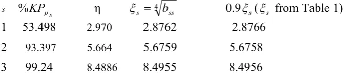
3.2 Plate with defect.
This case will test the inverse methodology by considering the case where the plate has some defect(s) such that its in the absence of fluid interaction natural frequencies, ξs, have all been reduced by 10%. In this case, once again, it will be assumed that such defect(s) do not incur significant change to the contents of the matrix K of equation (28). Therefore, the same form of the eigenfunction, equation (3), is used with the original values ofξsto generate the values of contained in equation (19). However values of
qs k
s
ξ reduced by 10% are used in the section
(
)
⎥⎥⎦⎤ ⎢
⎢ ⎣ ⎡
− −
q q
s α α
ρ η
ξ
tan 1
4 4
of equation (21) and the inverse process described in Section 3.1 is
repeated. In addition, in order to arrange that there will exist strong coupling between the first modes of the plate and fluid cavity as with the examples so far, for this case the non-dimensional depth of the fluid cavity is, from equation (24), c
s p
L = 8.2934. Table 5 lists the results for this test.
s %KP ξ =4 b ss
s 0.9ξs(ξs from Table 1) 1 53.498 2.970 2.8762 2.8766
[image:17.595.62.408.487.562.2]2 93.397 5.664 5.6759 5.6758 3 99.24 8.4886 8.4955 8.4956
Table 5 Comparison for a plate with defect reducing natural frequencies, ξs, by 10%.
From Table 5 it is seen that the method performs extremely well for the case where the plate has defect(s) giving rise to reductions in natural frequency from the undamaged plate values, and the matrices K and B from equations (28) and (29) respectively are generated using the eigenfunctions of equation (3) for the plate in the undamaged state.
4. CONCLUSIONS.
successful VHM procedures. This is an important step towards the development of practically applied vibration health monitoring methods. The paper presents a unique attempt to analytically characterize the vibration response of the coupled structure/fluid system and extract rather precisely the pure structural natural frequencies from those of the interacting system.
5. REFERENCES.
[1].Doebling S.W., C.R. Farrar and M.B. Prime, ”A Summary Review of Vibration-based Identification Methods”, Shock and Vibration Digest, 1998, 205(5), 631-545.
[2].Lenaerts W, Kerschen G and Golinval J C: ECL benchmark: Application of the proper orthogonal decomposition. Mechanical Systems and Signal Processing, 2003, 17(1), pp 237-242.
[3].Trendafilova I., Manoach E.,. Cartmell M.P,. Krawczuk M,. Ostachowicz W.M, Palacz M., On the Problem for Damage Detection of Vibrating Cracked Plates, 2006, Applied Mechanics and Materials 5-6, pp 247-254.
[4].Gorman D G, Reese J M, Horáček J and Dedouch K: Vibration analysis of a circular disc backed by a cylindrical cavity. Proceedings of the Institution of Mechanical Engineers, Part C, 2001, 215, pp1303-1311.
[5].Leissa, A.W.: Vibration of Plates. NASA SP-160, Washington, 1969.
[6].McLachlan, N.W.: Bessel Functions for Engineers. Oxford Engineering Science Series,1948,(Oxford University Press, London).
[7].Press, W.H, Flannery, B.P., Teukolsky, S.A., and Vetterling, W.T.: Numerical Recipes, Cambridge University Press, 1988, pp. 31-39.