A comparative study on mean value modelling of two-stroke marine diesel engine

A Comparative Study on Mean Value Modelling

of Two-Stroke Marine Diesel Engine

G. P. Theotokatos

Department of Naval Architecture

School of Technological Applications, TEI of Athens

St. Spyridonos Str., 12210 Egaleo, GREECE

mtheot@teiath.gr

http://www.na.teiath.gr

Abstract: -. In the present paper, two mean value modelling approaches of varying complexity, capable of simulating two-stroke marine Diesel engines, are presented. Both approaches were implemented in the computational environment of MATLAB Simulink®. Simulation runs of transient operation cases of a large two-stroke marine Diesel engine were performed. The derived results were validated against previously published data are used for comparing the two modelling approaches and discussing the advantages and drawbacks of each.

Key-Words: - mean value modelling, marine Diesel engine, simulation, MATLAB Simulink®

1 Introduction

Due to the very high cost for the procurement of the installation of a marine two-stroke Diesel engine, the major part of the engine control system development relies on appropriate simulation tools of varying complexity, which can be categorized as transfer function models, cycle mean value models and zero or one-dimensional models. The representation of the real engine processes is enhanced as the complexity of the used simulation tool is increased (i.e. from transfer function models to one-dimensional models), but at the same time, the required amount of input data as well as the model execution time is also increased. The cycle mean value models compromise between the above mentioned contradictory factors and, therefore, are widely used throughout the control system design procedure due to their simplicity and their ability to sufficiently represent the engine components behaviour [1,2].

In the present paper, two different ways of modelling a large two-stroke marine Diesel engine using cycle mean value models are presented. According to the first approach, the engine crankshaft and turbocharger shaft speeds are obtained by solving the angular momentum conservation differential equations. The other engine variables are obtained as solutions to a nonlinear algebraic system of three equations corresponding to energy and mass conservation across the engine. According to the second approach, the engine scavenging

and exhaust receivers are modelled as open

thermodynamic systems. The mass, temperature and pressure of the working medium contained in the engine receivers are calculated using the mass and energy differential equations and the ideal gas law, respectively. For representing the engine turbocharger compressor and turbine, their maps, derived under steady state conditions are used. The engine cylinders are modelled using a cycle mean value modelling approach to calculate the average mass flow and enthalpy rates of the exhaust gas exiting the cylinders and entering the exhaust receiver. Engine crankshaft and turbocharger shaft speeds are obtained using angular momentum conservation. The simulation

results from both modelling approaches are validated against previously published data. In addition, they are compared against each other leading to conclusions on each approach advantages and disadvantages.

2 Mean Value Engine Modelling

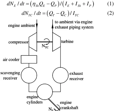
The two-stroke marine Diesel engine mean value engine model is constructed by considering the processes occurring in its components. The main engine components that have been mathematically modelled, shown in Fig. 1, are the cylinders, the scavenging and exhaust receivers, the compressor and turbine of the turbocharger and the engine air cooler. In addition, the engine exhaust pipe and the air filter, located upstream compressor, are also modelled.

In both mean value engine modelling (MVEM) approaches presented bellow, the engine crankshaft and turbocharger shaft speeds are calculated using the following equations derived by applying the angular momentum conservation in the propulsion plant shaft system and the turbocharger shaft, respectively:

(

) (

)

/ /

E Sh E P E Sh P

dN dt= η Q −Q I +I +I (1)

(

)

/ /

TC T C TC

dN dt= Q −Q I (2)

engine ambient

compressor

air cooler

exhaust receiver

NE

NTC

engine cylinders

to ambient via engine exhaust piping system

engine crankshaft

turbine

scavenging receiver

engine ambient

compressor

air cooler

exhaust receiver

NE

NTC

engine cylinders

to ambient via engine exhaust piping system

engine crankshaft

turbine

scavenging receiver

The engine cylinders of a two-stroke marine Diesel engine are modelled considering a system comprising two orifices connected in series. Each one of the orifices represents the cylinder intake ports and exhaust valve, respectively. These two orifices can be combined in one equivalent orifice producing the same mass flow rate for a given pressure ratio across engine cylinders and its geometric area can be estimated using the areas of intake ports and exhaust valves, as follows [3]:

(

)

(

)

0

/ 2π ( ) ( ) / ( ) ( ) d

eq cyl i e i e

A = z

∫

The cylinders air mass flow rate is calculated using the following equation, which has been derived according to the quasi-one dimensional consideration in an orifice with subsonic flow [4]:

(

)

(

)

(

)

(

)

/ , , / ,

, 2 / 1

a d eq SC a SC cyl cyl ER SC

cyl cyl cyl

m c A p R T f pr pr p p

f pr pr α pr α α

α

γ γ

γ

α α α

γ

γ γ γ +

= =

= _ − _ −

(4)

The mass and energy balances applied on engine cylinders give:

a f e

m +m =m (5)

(m ha SC +ηcombm Hf Lζ η) ex =m he ER (6)

where, ζ is fuel chemical energy proportion in the exhaust

gas entering turbine [3] and ηex is a correction factor used

to take into account the heat transfer from the exhaust gas to the ambient in the cylinder exhaust ports and exhaust receiver.

The proportion of the fuel chemical energy contained in the exhaust gas is considered linear function of the engine mean effective pressure [3]:

0 1

z z b

k k p

ζ = + (7)

The engine brake mean effective pressure is calculated by subtracting the friction mean effective pressure from the indicated mean effective pressure:

b i f

p =p −p (8)

The indicated mean effective pressure is calculated using the rack position, the maximum indicated mean effective pressure of the engine and the combustion efficiency, which in turn is regarded as function of air to fuel ratio [5]:

,max

i r i comb

p =x p η (9)

The friction mean effective pressure is considered function of the indicated mean effective pressure and the engine crankshaft speed [6,7]:

0 1 2

f f f E f i

p =k +k N +k p (10)

The engine fuel mass flow rate is calculated using the following equation, where of the injected fuel mass per cylinder and per cycle vs. fuel rack position is provided as input:

(

)

, / 60

f cyl f cy E cy

m =z m N rev (11)

The engine torque, brake power, brake specific fuel consumption and efficiency are calculated using the following equations:

, , ,

2 30

f

b D E E b

E b b

cy b f L

m

p V Q N P

Q P bsfc

rev P m H

π _η

π

= = = =

(12)

It must be noted that using the equations given above

the average (per cycle) values of engine parameters are calculated. In that respect, mean value modelling approaches can not be used for calculating the instantaneous values (per degree of crank angle) of the engine parameters.

The engine governor is modelled using a proportional-integral (PI) controller law. Thus, the engine governor rack position is calculated as follows:

, ₀

t

r r o p i

x =x + ∆ +k N k

∫

where ∆N=Nord-NE is the difference between the ordered

engine speed and the actual engine speed. In addition, torque and scavenging pressure limiters have been also incorporated in the engine governor model as proposed and used by engine manufacturers [8] for protecting the engine integrity during fast transients.

The compressor impeller absorbed and turbine wheel delivered torques, required in equation (2), are calculated by:

30 / , 30 /

C C TC T T TC

Q = P πN Q = P πN (14)

The compressor and turbine powers, absorbed and delivered to the turbocharger shaft respectively, are calculated depending on the modeling approach as described in the next sections of this text.

For modelling the air cooler, its effectiveness and pressure drop are required. The air cooler effectiveness is assumed to be a polynomial function of the air mass flow rate, according to the following equation:

2

0 1 2

AC kAC kAC ma kAC ma

ε = + + (15)

whereas the pressure drop in the air cooler is calculated by:

(

)

(

)

/ 2 / 2

AC AC AC AC a AC AC

p f ρ w f m ρ A

∆ = = (16)

The pressure after the turbine is calculated using the pressure increase of the exhaust piping system, which in turn is regarded as proportional to the exhaust gas mass flow rate squared:

2 ,

T d atm ep atm ep e

p =p + ∆p =p +k m (17)

The propeller torque, required in eq. (1), is calculated according to the propeller law through the engine maximum continuous rating (MCR) operating point:

2 2

, ,

, /

P P E P E MCR E MCR

Q =k N k =Q N (18)

2.1 1st MVEM Approach

The air and gas properties are considered to be constant. Thus, the temperature of the working medium (air or gas) throughout the engine components is calculated using the following equation:

p

h=c T (19)

efficiency parabola. In that respect, the compressor pressure ratio can be modelled as function of the turbocharger shaft speed, whereas the compressor efficiency can be taken either as constant or on the optimum efficiency curve of the compressor map.

According to the modelling approach presented in this section, the compressor pressure ratio and efficiency are regarded as second order polynomial functions of the turbocharger shaft speed and are calculated using the following equations:

2

1 2

1

C C TC C TC

pr = +k N +k N (20)

2

0 1 2

C kCef kCef NTC kCef NTC

η = + + (21)

The compressor exiting air temperature is calculated using the following equation, which has been derived using the compressor efficiency definition equation [5]:

( )

(

)

(

)

1 a 1 /

C a C C

T =T + pr γ − γα − η ₍₂₂₎

The pressure and temperature of the air contained in the engine scavenging receiver are derived as follows:

(

)

SC C AC AC w AC

T =T −ε +ε T (23)

SC C AC C atm AC

p =p − ∆p =pr p − ∆p (24)

The engine exhaust gas mass flow rate is calculated by the following equation derived applying a quasi-one dimensional approach [4,5] in the turbine:

( )

(

)

(

)

max / , 2 /( 1)

e e e e e e ER

e T eff T T

e e ER

T T d ex e

p

m A pr pr

R T

pr p p

γ γ γ γ γ γ γ γ + − = − −   = _ + _   (25)

The turbine effective flow area is calculated from the turbine geometric area and the turbine flow coefficient. The turbine flow coefficient and efficiency are derived from turbine steady state performance maps and are considered polynomial functions of the turbine pressure ratio, i.e.:

, , , ( ), ( )

T eff T T geo T T T T

A =α A α = f pr η = f pr (26)

Combining the equations (4)-(11), (15)-(17) and (19)-26), for a given set of engine speed, turbocharger

shaft speed and engine governor rack position, (NE, NTC,

xr), a non-linear algebraic system is solved to obtain the

three independent variables, i.e. the air mass flow rate, the exhaust receiver pressure, and the exhaust receiver temperature. Then, the remaining engine parameters are calculated from the respective equations given above.

Taking into account eq. (19), the power of compressor and turbine required according to eq. (2) and (14) for calculating turbocharger shaft speed, are calculated by:

(

)

(

)

C a pa C atm T e pe ER T d

P =m c T −T P =m c T −T (27)

where, the temperature of the exhaust gas exiting turbine is calculated using the following equation, which is derived by the turbine efficiency definition equation [5]:

(

)

(

)

, 1 1 , /

e e

T d ER T T d ER

T =T −η _ − p p γ− γ _

  (28)

The above presented equations were implemented in the MATLAB/Simulink® environment. The calculation procedure takes place as follows. At the start of the

simulation time, the values for the three independent variables (air mass flow rate, exhaust gas pressure and temperature) are initialized. For each time step, taking into account the values for engine speed, turbocharger shaft speed (their initial values are taken into consideration at the start of the simulation time) and rack position, the required engine parameters are calculated and the no-linear algebraic system is solved to provide the air mass flow rate and the exhaust gas pressure and temperature. Then, the remaining engine parameters, as well as the time derivatives of the engine speed and the turbocharger shaft speed are also derived. The engine speed and the turbocharger shaft speed are calculated using a fourth order Runge-Kutta integration method with fixed time step. The above described procedure is repeated for every time step till the end of the simulation time.

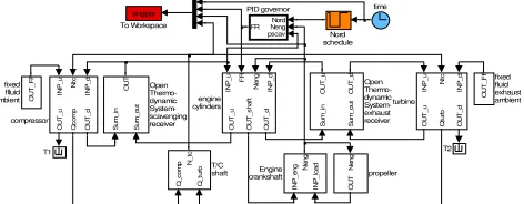
2.2 2nd MVEM Approach

According to the second modelling approach, the two-stroke marine Diesel engine is modelled using flow receivers (control volumes) interconnected between flow elements. Fixed fluid elements with constant pressure and temperature are used for modelling the engine boundaries. Shaft elements are used for calculating the engine crankshaft and turbocharger shaft rotational speeds by solving the differential equations (1) and (2), respectively. The engine governor rack position and propeller torque are calculated using equations (13) and (18) in the PI governor and propeller elements, respectively.

The engine scavenging and exhaust receivers are modelled as flow receivers, whereas the engine compressor, cylinders and turbine are modelled as flow elements. The model was also implemented in the MATLAB/Simulink environment following a modular way as shown in Figure 2. Thus, the modelled engine elements form discrete subsystems, which exchange the required variables through appropriate connections. The flow elements use as input the pressure, temperature and the properties of the working medium (air or gas) contained in the adjacent elements (flow receiver(s) or fixed fluid), whereas their output includes the mass flow and energy rates entering and exiting the flow element as well as the absorbed (for the case of compressor) or produced torques. The former are provided as input in the adjacent flow receiver elements, whereas the latter is required as input in the shaft elements. The output of shaft elements i.e. the engine crankshaft and turbocharger

IN P _ u N tc IN P _ d O U T _ u Q tu rb O U T _ d turbine time N e n g O U T propeller O U T _ F F _fixed fluid exhaust ambient O U T _ F F fixed flluid ambient IN P _ u F R N e n g IN P _ d O U T _ u O U T _ s h a ft O U T _ d engine cylinders engpar To Workspace T2 T1 Q _ c o m p Q _ tu rb N _ tc T/C shaft Nord Neng pscav FR PID governor S u m _ in S u m _ o u t O U T _ u O U T _ d Open Thermo-dynamic System- exhaust receiver S u m _ in S u m _ o u t O U T Open Thermo-dynamic System-scavenging receiver Nord schedule IN P _ e n g IN P _ lo a d N e n g Engine crankshaft IN P _ u N tc IN P _ d O U T _ u Q c o m p O U T _ d compressor

shaft rotational speeds, are supplied as input in the respective flow controller.

The flow receiver elements are modelled using the open thermodynamic system concept [4,5]. The working medium mass, temperature and pressure are calculated using the following equations derived from mass and energy balances and the ideal gas law, respectively:

/ in out

dm dt=m −m (29)

(

)

(

)

/ ht in in out out / / v

dT dt= Q +m h −m h −udm dt mc (30)

/

p=mRT V (31)

No heat transfer is taken into account for the scavenging receiver, whereas the transferred heat from the gas contained in the exhaust receiver to the ambient is calculated using the following equation:

(

)

ht ht ht ER atm

Q =k A T −T (32)

The working medium properties are considered to be functions of temperature and fuel to air equivalence ratio. The compressor is modelled using its steady state performance map, which is provided as input in a digitized form containing lines of the turbocharger speed, pressure ratio, corrected flow rate and efficiency. Given the turbocharger speed and pressure ratio, the corrected

flow rate and efficiency are calculated using

interpolation. The compressor pressure ratio is calculated by the following equation using the pressures of the fixed fluid and the scavenging receiver connected upstream and downstream the compressor, respectively, the pressure drops in the air filter and air cooler and the pressure increase in the auxiliary blower:

(

) (

)

C SC AC BL atm AF

pr = p − ∆p + ∆p p − ∆p (32)

The air filter pressure drop is considered to be function of the compressor mass flow rate as follows:

2

AF AF C

p k m

∆ = (33)

The blower pressure increase is taken as function of the volumetric flow rate:

( )

BL BL

p f V

∆ = (34)

The air cooler is modelled using eq. (15) and (16). The temperature of the air exiting the compressor is calculated using eq. (22). The compressor absorbed power is calculated by:

(

)

C C C atm

P =m h −h (35)

where the enthalpies of the air exiting and entering the

compressor are calculated from the respective

temperatures.

The turbine is modelled using its swallowing capacity and efficiency maps, which must be provided in digitized form. Given the turbine pressure ratio, the turbine mass flow rate and efficiency are calculated using interpolation. The temperature of the gas exiting turbine is calculated by equation (28). The turbine power is derived by:

(

)

T T ER T d

P =m h −h (36)

The model includes six differential equations (eq. (29),(30) for engine scavenging and exhaust receivers and eq. (1),(2)), which are solved using a fourth order Runge-Kutta integration method with fixed time step.

3 Results and Discussion

The above described MVEM approaches were applied for examining the transient behaviour of the MAN B&W 9K90MC two-stroke marine Diesel engine. That engine was also used in previous research studies [8-10], where significant amount of experimental data and simulation results were published. The main engine characteristics as well as the required input data and engine steady state performance data were extracted from the engine manufacturer project guide [11].

For each one of the MVEM approaches, the following steps were followed. Initially, the mean value engine model was set up and the required constants were calibrated so as the simulation results under steady state conditions are in good agreement with the respective ones presented by the engine manufacturer in [11]. Then, the calibrated mean value engine model was used to perform simulation runs under engine transient operating conditions.

The transient engine operation case selected to be investigated was the first one presented in [8]. According to that, the engine operation for 100 seconds with changes of the ordered engine speed from 94 rpm to 69 rpm at the

10th sec and back to 94 rpm at 60th sec was examined. The

changes in ordered speed correspond to engine load changes from 100% load to 40% load. Such changes are considered very abrupt and are usually avoided in real engine operation, but engine operation response under similar load changes are used for the control system design. The results for the above mentioned transient run presented in [8] were derived using a zero-dimensional engine simulation code, which was extensively validated under steady state and transient conditions [8-10] and, therefore, are considered of high reliability. So, they are used in the Fig. 3 and 4 presented below as “reference” data.

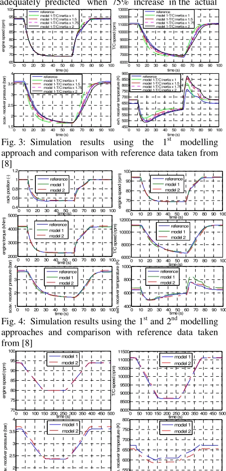
A set of results derived using the 1st MVEM

approach, including the engine crankshaft speed, the turbocharger shaft speed, the scavenging receiver pressure and the exhaust receiver temperature are shown in Fig. 3 (labelled as “model 1–T/C Inertia x 1”). As it is deduced from Fig. 3, the engine speed response is adequately predicted during the first applied ordered

speed change (after the 10th sec). However, there is a

slight deviation between the predictions for the engine speed and the respective reference data during the second

applied ordered speed change (after 60th sec), where,

according to the predictions, the scavenging pressure limiter is not engaged as it occurs in the reference case. That is explained as follows. As it is shown in Fig. 3, the

turbocharger speed, predicted using the 1st MVEM

approach, varies more rapidly than the respective one of the reference case, owing to the unmodelled dynamic of the scavenging and exhaust receivers’ volumes. Thus, the predicted scavenging receiver pressure during the second

ordered speed change (after 60th sec) was greater than the

between the predictions and the reference data.

A way to improve the model accuracy is through increasing the value of the turbocharger rotating parts polar moment of inertia by an additional quantity. That added inertia corresponds to the turbocharging system volume inertia (scavenging and exhaust receiver volumes, compressor and turbine piping). The simulation run was repeated increasing the actual value of the turbocharger polar moment of inertia by 50%, 75% and 100%. The respective results are also presented in Fig. 3. As it is shown in Fig. 3, the responses of the engine speed, turbocharger speed and scavenging receiver pressure are adequately predicted when 75% increase in the actual

0 10 20 30 40 50 60 70 80 90 100 65 70 75 80 85 90 95 100 time (s) e n g in e s p e e d ( rp m ) reference model 1-T/C inertia x 1 model 1-T/C inertia x 1.5 model 1-T/C inertia x 1.75 model 1-T/C inertia x 2

0 10 20 30 40 50 60 70 80 90 100 6000 7000 8000 9000 10000 11000 12000 13000 time (s) T /C s p e e d ( rp m ) reference model 1-T/C inertia x 1 model 1-T/C inertia x 1.5 model 1-T/C inertia x 1.75 model 1-T/C inertia x 2

0 10 20 30 40 50 60 70 80 90 100 1.5 2 2.5 3 3.5 4 time (s) s c a v . re c e iv e r p re s s u re ( b a r) reference model 1-T/C inertia x 1 model 1-T/C inertia x 1.5 model 1-T/C inertia x 1.75 model 1-T/C inertia x 2

0 10 20 30 40 50 60 70 80 90 100 450 500 550 600 650 700 750 800 850 900 time (s) e x h . re c e iv e r te m p e ra tu re ( K ) reference model 1-T/C inertia x 1 model 1-T/C inertia x 1.5 model 1-T/C inertia x 1.75 model 1-T/C inertia x 2

Fig. 3: Simulation results using the 1st modelling

approach and comparison with reference data taken from [8]

0 10 20 30 40 50 60 70 80 90 100 0.4 0.6 0.8 1 1.2 time (s) ra c k p o s iti o n ( -) reference model 1 model 2

0 10 20 30 40 50 60 70 80 90 100 60 70 80 90 100 time (s) e n g in e s p e e d ( rp m ) reference model 1 model 2

0 10 20 30 40 50 60 70 80 90 100 2000 3000 4000 5000 time (s) e n g in e t o rq u e ( k N m ) reference model 1 model 2

0 10 20 30 40 50 60 70 80 90 100 6000 8000 10000 12000 time (s) T /C s p e e d ( rp m ) reference model 1 model 2

0 10 20 30 40 50 60 70 80 90 100 1 2 3 4 time (s) s c a v . re c e iv e r p re s s u re ( b a r) reference model 1 model 2

0 10 20 30 40 50 60 70 80 90 100 400 600 800 1000 time (s) e x h . re c e iv e r te m p e ra tu re ( K ) reference model 1 model 2

Fig. 4: Simulation results using the 1st and 2nd modelling

approaches and comparison with reference data taken from [8]

0 50 100 150 200 250 300 350 400 450 500 70 75 80 85 90 95 100 time (s) e n g in e s p e e d ( rp m ) model 1 model 2

0 50 100 150 200 250 300 350 400 450 500 8000 8500 9000 9500 10000 10500 11000 11500 time (s) T /C s p e e d ( rp m ) model 1 model 2

0 50 100 150 200 250 300 350 400 450 500 1.5 2 2.5 3 3.5 4 time (s) s c a v . re c e iv e r p re s s u re ( b a

r) model 1

model 2

0 50 100 150 200 250 300 350 400 450 500 500 550 600 650 700 750 800 time (s) e x h . re c e iv e r te m p e ra tu re ( K

) _{model 1}

model 2

Fig. 5: Simulation results using the 1st and 2nd modelling

approaches for a slow engine transient operation case

value of the turbocharger polar moment of inertia is used. On the contrary, the prediction of the exhaust receiver temperature exhibits greater deviation from the respective reference data.

A set of simulation results derived from a) the 1st

MVEM approach using 75% increase in the actual value of the turbocharger polar moment of inertia (model 1), b)

the 2nd MVEM approach (model 2) and the respective

reference data (reference) are presented in Fig. 4. As it is observed from Fig. 4, the engine parameters response including the exhaust receiver temperature are predicted

with very satisfactory accuracy using the 2nd MVEM

approach. This is attributed to the more detailed modelling of engine receivers and, in a lesser extent, to the use of complete compressor map. Adequate agreement in the prediction of engine parameters (except from exhaust receiver temperature) is also obtained using

the 1st MVEM approach. The execution time of the

simulation run using the 2nd MVEM approach increased

in comparison to the respective one of the 1st _MVEM

approach, but it was reasonable. Thus, the 2nd MVEM

approach can be reliably used in advanced engine control studies, e.g. including, apart from engine speed control, turbocharger speed or scavenging receiver pressure control etc.

However, in cases of slow engine transients, which are usual for the ship propulsion plant operation, the engine parameters are also predicted with enough

accuracy using the 1st MVEM approach, as inferred by

comparing the results shown in Fig. 5, which are derived

from a slow transient run conducted with 1st and 2nd

MVEM approaches.

4 Conclusions

The modelling of a large two-stroke marine Diesel engine was presented by using two different mean value approaches. The simulation results were used for revealing the advantages and drawbacks of each approach.

The main findings derived from this work are summarised as follows.

The first mean value engine model is simpler, requires smaller amount of input data and takes less computing time for execution. It adequately predicts the engine speed response and in that respect, it can be reliably used in the engine speed control design process. In order to represent with acceptable accuracy the turbocharger shaft speed response during fast transients, the value of the turbocharger rotating parts polar moment of inertia, provided to the model as input, must be increased by an additional amount for taking into account the effect of the volume inertia of the engine scavenging and exhaust receivers. In such a case, additional data (experimental data or simulation results from more detailed models) are required in order to adjust the value of turbocharger inertia. Thus, for advanced engine control studies (e.g. including, apart from engine speed control, turbocharger speed or scavenging receiver pressure control), such a model should be carefully treated.

additional input data, including the compressor and turbine maps, the volume of the engine receivers and initial values for the pressure and temperature of the gas contained in the engine receivers. The engine physical processes are more accurately represented since the second approach includes the more detailed modelling of the engine scavenging and exhaust receivers. In that respect, the model gives better predictions for the engine operating parameters response during fast transients. In addition, the model execution time, although greater than the respective one of the first model, is reasonable enough. As a result, the second modelling approach is more appropriate for advanced engine control system design studies.

References:

[1] Guzzella L. and Onder Ch.H., “Introduction to Modeling and Control of IC Engine Systems”, Springer, 2007.

[2] Eriksson L., “Modeling and Control of Turbocharged SI and DI engines”, Oil & Gas Science and Technology-Rev. IFP, Vol.62, No. 4, pp. 523-538, 2007.

[3] Meier E., “A Simple Method of Calculation and Matching Turbochargers”, BBC Brown Boveri & Company Ltd, Publication No. CH-T 120 163 E.

[4] Heywood J.B, “Internal Combustion Engines

Fundamentals”, Mc-Graw Hill, 1988.

[5] Watson N., and Janota M. S., “Turbocharging the Internal Combustion Engine”, Macmillan Press, 1982. [6] Theotokatos G., “A Modelling Approach for the Overall Ship Propulsion Plant Simulation”, 6th WSEAS International Conference on System Science and Simulation in Engineering (ICOSSSE ’07), November 21-23, Venice, Italy, 2007.

[7] Xiros N., “Robust Control of Diesel Ship Propulsion”, Springer, 2002.

[8] Kyrtatos N.P., Theodossopoulos P., Theotokatos G., Xiros N., “Simulation of the overall ship propulsion plant for performance prediction and control”, MarPower99 Conference, Newcastle upon Tyne, UK, 1999.

[9] Kyrtatos N.P., Theotokatos G., Xiros N., Marec K., and Duge R., “Transient Operation of Large-bore Two-stroke Marine Diesel Engine Powerplants: Measurements and Simulations”, 23rd CIMAC World Congress, Hamburg, Germany, 2001.

[10] Kyrtatos N.P., Theotokatos G., and Xiros N.I., (2002), “A Virtual Experiment Tool for Marine Diesel Engine Powerplant Analysis”, IMAM 2002, Rethymnon, Crete, Greece, May 13-17, 2002.

[11] MAN B&W, K90MC Mark 6 Project Guide Two-Stroke Engines, 5th Edition, November 2000.

NOMENCLATURE

A : area

bsfc: brake specific fuel consumption

cd : discharge coefficient

cp : specific heat at constant pressure

cv : specific heat at constant volume

f : friction factor, fuel

Ι : polar moment of inertia

HL : fuel lower heating value

h : specific enthalpy

k : coefficients, constants

m : mass

m : mass flow rate

N : rotational speed

P : power

p : pressure

pr : pressure ratio

p : mean effective pressure

Q : torque

R : gas constant

revcy: revolutions per cycle

T : temperature

t : time

u : specific internal energy

VD : displacement volume

w : velocity

xr : rack position

zcyl : number of engine cylinders

αT : turbine flow coefficient

γ : ratio of specific heats

∆p : pressure drop

ε : effectiveness

η : efficiency

ηex: correction factor for the temperature of the

exhaust receiver

ρ : density

ζ : proportion of the chemical energy of the fuel

contained in the exhaust gas

φ : crank angle

Subscripts

AC : air cooler AF : air filter atm : ambient BL : blower b : brake C : compressor comb: combustion cy : cycle

cyl: cylinder d : downstream E: engine

ER : exhaust receiver e: exhaust gas, exhaust valve ep : exhaust pipe

eq : equivalent f : fuel, friction ht : heat transfer i : indicated, intake ports MCR : maximum continuous rating

o : initial conditions

P : propeller

SC : scavenging receiver Sh : shaft