A study into the behaviour of the formation level of an excavation under different unloading patterns in soft deposits

City, University of London Institutional Repository

Citation

:

This is the accepted version of the paper.

This version of the publication may differ from the final published

version.

Permanent repository link:

Link to published version

:

Copyright and reuse:

City Research Online aims to make research

outputs of City, University of London available to a wider audience.

Copyright and Moral Rights remain with the author(s) and/or copyright

holders. URLs from City Research Online may be freely distributed and

linked to.

A study into the behaviour of the formation level of an excavation

under different unloading patterns in soft deposits

Yuqi Li1, *, Xiaohui Chen1, Sam Divall2, Xiaodi Zhang1

1 Department of Civil Engineering, Shanghai University, Shanghai 200072, China

2 Department of Civil Engineering, City University London, London EC1V 0HB, UK

*

Corresponding author: [email protected]

Abstract：The construction of basements in urban areas is often associated with the possible damage to existing structures and services. The varying construction processes inevitably lead to different stress unloading

patterns and therefore the dissipation of these excess pore-water pressures may lead to non-standard deformation

profiles. The three main types of basement construction processes are Layered Excavation (LE), Basin Excavation

(BE) and Island Excavation (IE). The effect of the various unloading patterns has been investigated by a three

dimensional (3D) effective stress analysis method using the developed computer program 3DBCPE4.0. An

excavation of length 50m, width 50m and depth 9m in a certain homogenous and isotropic saturated soft soil was

modelled. This included a diaphragm wall of 800mm thickness embedded 18m deep into the soft soil. The

different excavation deformation profiles under different excavation patterns were related to the different

unloading process, the exposure time of excavation face and the dissipation of negative excess pore-water

pressures. The most favourable process for controlling the horizontal deformation of a retaining wall or the heave

deformation of the formation level is suggested. The ground water potentials within the formation level are also

presented.

1. Introduction

Excavation will cause the deformations of retaining structure, pit base and ground surface,

therefore, numerous investigations on the characteristics of excavation-induced deformations have

been performed. Ou and his research group did a lot of research, they proposed an empirical

method for predicting the spandrel and concave settlement profiles on the basis of a regression

analysis of the field observations of settlement curves (Hsieh and Ou, 1998), studied building

responses and ground movements caused by an excavation using the top-down construction

method (Ou et al., 2000), analysed basal heave of excavations (Hsieh et al., 2008), evaluated basal

heave stability (Do et al., 2013), and investigated extensively the behaviour of excavations with

cross walls (Hsieh et al., 2012; Hsieh et al., 2013; Ou et al., 2013; Wu et al.,2013). In addition,

Zdravkovic et al. (2005), Kung et al. (2007a; 2007b) and Finno et al. (2007) studied the

deformation behaviour of excavation in other aspects.

Excavation will also cause the variation of pore pressure due to unloading. In order to

investigate variation of pore-water pressure induced by excavation, 3D effective stress analysis

based on Biot’s consolidation theory was performed. Osaimi and Clough (1979) investigated

pore-water pressure dissipation during an excavation based on Biot’s consolidation theory.

Benmebarek et al. (2006) analysed the effect of seepage flow on the lateral earth pressures acting

on deep sheet piled wall excavations in cohesionless soil using the explicit finite difference

method implemented in Fast Lagrangian Analysis of Continua (FLAC) code. The distribution

rules of the formation level deformations and excess pore-water pressure were analysed in detail

integrating the time parameter by Li et al. (2008). Borges and Guerra (2014) analysed the

investigated the influence of the diameter of excavation, the embedded length of the wall and the

elastic modulus of the wall material on the behaviour of the formation level.

In actual engineering, there are different excavation patterns according to the surrounding

environment and the stability of excavation. LE is that soil is excavated uniformly from the

excavation, BE is that the soil at the formation level centre is excavated first whereas the soil

around the formation level centre is excavated later, and IE refers to that the soil around the

formation level centre is excavated first whereas the soil at the formation level centre is excavated

later. However, as reported above, little work has focused on the effect of the excavation patterns

(such as IE and BE) on the formation level. Tan and Wang (2013a; 2013b) studied the

characteristics of a circular excavation and its peripheral according to a large-scale deep

excavations by the Island technique. The study compared bottom-up construction of the central

cylindrical shaft first and top-down construction of the peripheral rectangular excavation in

Shanghai’s soft clay. However, they concentrated on formation level shape (central circular and

peripheral rectangular) and the construction method (bottom-up construction and top-down

construction) via the analysis of formation level deformations.

In this study, to explore the effects of excavation patterns on the behaviour of the formation

level, based on Biot’s consolidation theory, a computer program 3DBCPE4.0 was developed by

3D FEM. This was used to perform the coupled analysis of soil mass deformation and pore-water

pressure dissipation. LE, BE and IE were modelled respectively and the results are reported in this

paper.

2. Biot’s 3D consolidation finite element equations

2002) can be written in the following form:

, -* + * + (1)

where [K] is the element consolidation matrix (a symmetric matrix of 32×32 since a mesh of eight

noded hexahedral isoparametric elements is used to discretize a pit geometry in this paper),

* + is the increment column matrix of unknown terms of element node and * + is the

increment column matrix of equivalent load and water runoff of element node.

The sub matrix of the , - matrix is given by:

[ ] [

[ ] [ ]

[ ] ] ( )

(2)

where is the integration constant which ranges from 0.5 to 1.0, [ ] is the sub matrix of

element stiffness matrix, [ ] is the sub matrix of element coupling matrix and is the

component of element seepage matrix (Xie and Zhou, 2002).

The sub matrices of the * + and * + matrices can be expressed respectively as:

* + , - ( ) (3)

* + , - ( ) (4)

where , 𝜐, , and are the displacement increments and the pore-water pressure

increment of the ith element node, respectively, , , and are the equivalent

load increments and the equivalent water runoff increment of the ith element node, respectively.

The seepage effect induced by the water head difference between the inside and the outside

of the formation level cannot be taken into account when analysing excavation deformation and

pore-water pressure using Eq.(1). Thus, a ground water potential is introduced for consolidation

analysis of the excavation. When neglecting the solute potential the ground water potential of a

(5)

where P is the ground water potential of a saturated soil, p is the sum of pressure potential

(hydrostatic pressure) and load potential (excess pore water pressure), i.e. the total pore-water

pressure, the spatial coordinate z is upwards positive, is unit weight of water, and z is the

gravity potential.

The ground water potentials of element node i at time 𝑛 and 𝑛+1 are represented by (𝑛)

and (𝑛+1), respectively. Thus Eqs.(3) and (4) may be written in the following form without

regard to the influence of soil vertical displacement:

* + , (𝑛+1)- ( )

* + [ ′ ′ ′ ′ ] ( )

(6)

(7)

where ′ [ ] (𝑛) , ′ , - (𝑛), ′ [ ] (𝑛) and

′ (𝑛).

Based on the finite element equations derived above, a 3D consolidation finite element

program 3DBCPE4.0 was developed. In order to validate the program, an analysis of

one-dimensional consolidation for homogeneous soft soils under time-dependent loading was

introduced (Li et al., 2008). The soil layer top is pervious and free, and the bottom is impervious

and fixed. Displacements perpendicular to the boundaries are restrained and an impermeable

condition is assigned at the vertical boundaries. Soil parameters are: Poisson’s ratio μ=0.301,

elasticity modulus E=3MPa, vertical permeability coefficient kv=1.0×10 8

m/s, and thickness of

soil layer H=10m. A load curve is shown in Fig.1 where maximum load q0=100kPa and time

t0=70d.

divided into 7 meshes, as shown in Fig.2.

Fig.1 Loading curve

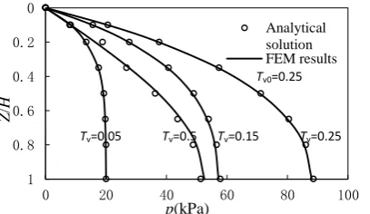
The comparisons of pore pressure, settlement

and average degree of consolidation between the

FEM results and the analytical solution of 1D

consolidation are shown in Figs.3 and 4. The

results of FEM agree very well with those of the

analytical solution, which proves the validity of the

program, so it can be used for effective stress analysis.

Fig.3 Comparison of pore pressure

(a) settlement (b) average degree of consolidation

Fig.4 Comparisons of settlement and average degree of consolidation

0 0.2 0.4 0.6 0.8 1

0 20 40 60 80 100

Analytical solution FEM results 0 10 20 30

0.01 0.1 1

Sct (cm ) T_v Analytical solution FEM results 0 20 40 60 80 100

0.01 0.1 1

U (%) T_v Analytical solution FEM results q q0

t0 t

o

Fig.2 Finite element mesh used for analysis of 1D consolidation

y z o x 1m 1m 1 .5 m 1 .5 m 2 m 1 .5 m 1 .5 m Tv0=0.25 Z / H p(kPa)

Tv=0.05 Tv=0.5 Tv=0.15 Tv=0.25

3. Stress-strain relationship of soil

Soil behaviour was simulated using the revised Duncan-Chang model (Duncan and Chang,

1970; Kulhawy and Duncan, 1972) in this paper. The model assumes a hyperbolic stress-strain

relationship and a variable Poisson’s ratio by means of stress-dependent Poisson’s ratio (Kulhawy

and Duncan, 1972).

The initial modulus is defined as:

. /𝑛 (8)

where the modulus number K and modulus exponent n are dimensionless material parameters; σ3

is the minor principal stress; pa is atmospheric pressure expressed in the same pressure units as σ3.

When the stress-strain relationship is employed in incremental form, the tangent modulus

corresponding to any point on a stress-strain curve can be expressed as:

0 ₊ (1 )( )1 . /𝑛 (9)

where c and φ are Mohr-Coulomb strength parameters; σ1 is the major principal stress; and Rf is

the failure ratio.

When (σ1–σ3) is less than its historical maximum, it is assumed that the soil is under

unloading or reloading and the tangent modulus is defined as:

. / 𝑛

(10)

where Kur is the unloading-reloading modulus number and is always greater than the primary

loading modulus number K.

The initial Poisson’s ratio can be expressed as:

. / (11)

(1 ) (12)

where ( )

.

/ 01 ( )( ) 1

; and D, F and G are material parameters.

4. Studies on the behaviour of foundation pit under different excavation patterns

4.1 Numerical example and finite element model

A formation level of length 50m, width 50m and depth 9m in a certain homogenous and

isotropic saturated soft soil is presented. The diaphragm wall of 800mm thickness is embedded

18m deep in soft soil. The groundwater tables inside and outside the excavation were assumed to

locate on the excavated surface and the ground surface respectively. Soil vertical and horizontal

permeability coefficients (i.e. kh and kv) are both 1.0×10−8m/s and the effective unit weight of soil

γ' is 9.0kN/m3 (Table 1).

Table 1 Soil parameters used during modelling

K n Rf c′ φ′ F G D Kur kh kv γ'

(kPa) (°) (m/s) (m/s) (kN/m3)

150 0.7 0.85 15 35 0.15 0.35 3.5 300 1.0×10-8 1.0×10-8 9

Two layer struts of reinforce concrete are respectively set at 3m and 6m under the ground

surface. Their cross-sectional dimensions at the first tier and the second tier were 600mm by

600mm and 600mm by 700mm, respectively. The horizontal spaces between the struts within the

excavation at every tier were 8.3m. Given that the influence scope of an excavation and the

symmetry about the formation level centreline, the dimensions of the model in x-, y- and

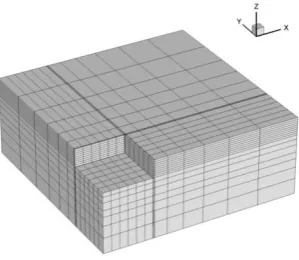
z-direction are 100m (length) by 100m (width) by 40m (depth). Finite element meshes of soil mass

and retaining wall are shown in Fig.5 wherein the element size was fine near the walls where

Fig.5 Mesh of finite elements

The bottom boundary of the excavation model was assumed to be fixed and displacements

perpendicular to the boundaries were restrained at the lateral boundaries. As far as the hydraulic

boundary conditions were concerned, a no-flow condition was assigned at the symmetrical plane

and an impermeable condition was assigned at the vertical boundaries. The bottom boundary of

the model was impermeable whereas the top was permeable and the retaining walls were

double-sided impermeable.

All soil units were discretized using eight-node hexahedral isoparametric elements and was

simulated using the revised Duncan-Chang model. According to the studies of many researchers

(Duncan and Chang, 1970; Kulhawy and Duncan, 1972; Ou et al.,1996; Liao, 2009), the

parameters of hyperbolic model in this paper are listed in Table 1. In Table 1 c' and φ' are the

effective cohesion and the effective internal friction angle of soil respectively. Retaining walls

were modelled with a linear elastic model whose modulus of elasticity and Poisson’s ratio are

25GPa and 0.167 respectively. Retaining wall’s elements were discretized using Wilson

non-harmony elements. A row of 0.1m thick interfaces were used to connect soil mass and

retaining wall elements. The two sides of the retaining wall adopted 3D thin interface elements

which were derived from Yin’s rigid plastic model (Yin et al., 1995) for outer friction angle=1.0°

mass elements. Supports were simulated with the linear elastic model with 23GPa elasticity

modulus and discretized using spatial bar elements.

4.2 Construction process under different excavation patterns

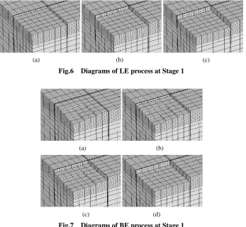
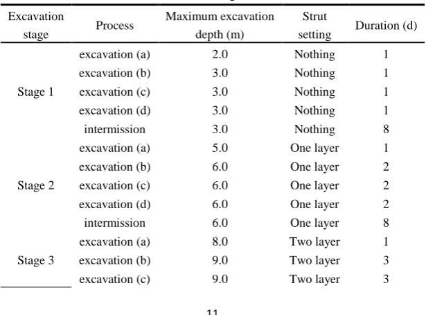
LE, BE and IE all involved three stages and the excavated thickness at every stage was 3m.

Construction at every stage was divided into three or four stages to complete (see Figs.6-8).

Excavation intermissions after every excavation stage were allowed for installation of struts or

casting the formation level base concrete. Excavation duration each stage and the intermission

duration after each stage under the different excavation patterns were also kept the same (as shown

in Tables 2-4).

(a) (b) (c)

Fig.6 Diagrams of LE process at Stage 1

(a) (b)

(c) (d)

(a) (b)

(c) (d)

Fig.8 Diagrams of IE process at Stage 1

Table 2 LE process

Excavation

stage Process

Excavation thickness (m)

Total excavation depth (m)

Strut

setting Duration (d)

Stage 1

excavation(a) 1.0 1.0 Nothing 1

excavation(b) 1.0 2.0 Nothing 1

excavation(c) 1.0 3.0 Nothing 2

intermission 0.0 3.0 Nothing 8

Stage 2

excavation(a) 1.0 4.0 One layer 2

excavation(b) 1.0 5.0 One layer 2

excavation(c) 1.0 6.0 One layer 3

intermission 0.0 6.0 One layer 8

Stage 3

excavation(a) 1.0 7.0 Two layer 3

excavation(b) 1.0 8.0 Two layer 3

excavation(c) 1.0 9.0 Two layer 4

intermission 0.0 9.0 Two layer 10

Note: excavation processes (a), (b) and (c) at the first stage are shown in Fig.6

Table 3 BE process

Excavation

stage Process

Maximum excavation depth (m)

Strut

setting Duration (d)

Stage 1

excavation (a) 2.0 Nothing 1

excavation (b) 3.0 Nothing 1

excavation (c) 3.0 Nothing 1

excavation (d) 3.0 Nothing 1

intermission 3.0 Nothing 8

Stage 2

excavation (a) 5.0 One layer 1

excavation (b) 6.0 One layer 2

excavation (c) 6.0 One layer 2

excavation (d) 6.0 One layer 2

intermission 6.0 One layer 8

Stage 3

excavation (a) 8.0 Two layer 1

excavation (b) 9.0 Two layer 3

excavation (d) 9.0 Two layer 3

intermission 9.0 Two layer 10

Note: excavation processes (a), (b), (c) and (d) at the first stage are shown in Fig.7

Table 4 IE process

Excavation

stage Process

Maximum excavation depth (m)

Strut

setting Duration (d)

Stage 1

excavation (a) 2.0 Nothing 1

excavation (b) 3.0 Nothing 1

excavation (c) 3.0 Nothing 1

excavation (d) 3.0 Nothing 1

intermission 3.0 Nothing 8

Stage 2

excavation (a) 5.0 One layer 1

excavation (b) 6.0 One layer 2

excavation (c) 6.0 One layer 2

excavation (d) 6.0 One layer 2

intermission 6.0 One layer 8

Stage 3

excavation (a) 8.0 Two layer 1

excavation (b) 9.0 Two layer 3

excavation (c) 9.0 Two layer 3

excavation (d) 9.0 Two layer 3

intermission 9.0 Two layer 10

Note: excavation processes (a), (b), (c) and (d) at the first stage are shown in Fig.8

4.3 Deformation behaviour of excavation

Excavations will cause the horizontal displacement of retaining walls, ground surface

settlements around the excavation and heave of the formation level. The excavation deformations

under LE, BE, and IE areanalysed and investigated by the comparison of the following:

1) The horizontal displacement of retaining wall,

2) The ground settlement around foundation pit, and

3) The heave of pit base.

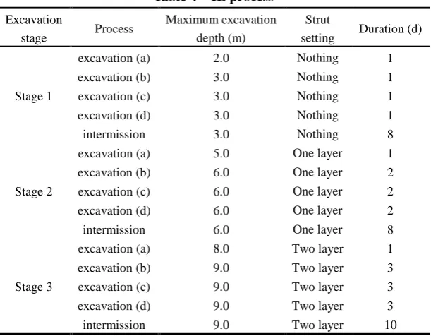
Fig.9 shows the horizontal displacement comparison at the x=0 section and at the third (final)

excavation stage. The maximum horizontal displacements under the different excavation patterns

all occur at approximately 2m under the excavation surface (i.e. 11m under the surface level). In

increases by 2.5% compared with LE. The different horizontal displacements of the retaining wall

under the excavation patterns were induced by changing the process of applying the earth pressure

acting on the retaining structure within the excavation. Take the first excavation stage, for example,

the exposure time of the retaining wall within the excavation at the end of the first excavation

intermission is shown in Table 5. The horizontal displacement comparison at the x=0 section and

at the end of the first excavation intermission is indicated in Fig.10. The retaining wall has a

cantilever-type deflection because the excavation was carried out without a strut installation at the

first stage. It can be seen from Table 5 and Fig.10 that the lateral displacements of the retaining

wall under BE are smaller than those under LE and IE. Since the exposure time of the retaining

structure was the shortest under BE (0-2m depth range) the duration that the lateral earth pressure

acting on the retaining wall inside the excavation was zero was the shortest. The moment acting

on retaining wall was induced by the lateral earth pressure outside the excavation at 0-2m depth

range which is larger than the one at 2-3m depth range. The duration that the lateral earth pressure

acting on the 2-3m depth range of retaining wall inside the excavation under IE was zero was

slightly larger than under LE leading to the lateral displacements of the retaining wall under IE

and LE being very close. Therefore, the soil around the retaining structure inside the excavation

under BE was excavated later and the exposure time of the retaining wall decreased. This was

Fig.9 Displacement of retaining structure at the third excavation stage

Fig.10 Displacement of retaining structure at the end of the first excavation intermission

Table 5 Exposure time of retaining wall

Depth range

of retaining wall BE (d) LE (d) IE (d)

0~1m 10 11 11

1~2m 9 10 10

2~3m 8 8 9

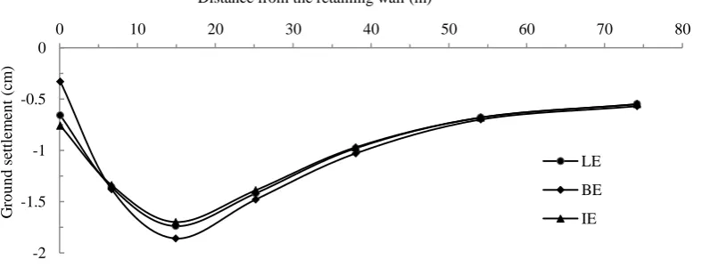
Fig.11 shows the ground surface settlement around the formation level at the x=0 section

under the three different excavation patterns after the third excavation stage. It can be seen from

Fig.11 that the maximum settlement occurred at 15m from the formation level and the settlement -18.0 -15.0 -12.0 -9.0 -6.0 -3.0 0.0

0 5 10 15 20 25 30 35 40 45 50 55

De

p

th

(m

)

Horizontal displacement of retaining structure (mm)

LE BE IE

-18.0 -15.0 -12.0 -9.0 -6.0 -3.0 0.0

0 5 10 15 20 25 30 35 40 45 50 55

D

ep

th

(m

)

Horizontal displacement of retaining structure (mm)

profiles were concave (similar to Hsieh &Ou, 1998). The excavation patterns have little influence

on the ground surface settlement. Within 6m from the formation level the settlement values, under

BE, were smaller than those of LE. IE had larger settlements because the wall deflection effects

the soil near the formation level. The wall displacements under BE were smaller than the ones

under LE and IE (Figs.9 and 10) and so the lateral pressures of the soil outside the excavation

under BE were larger. The vertical stress of the soil outside the excavation under the three

construction patterns were approximately the same, i.e. the smaller horizontal displacement means

the larger confining pressure of the soil outside the excavation. This will inhibit the settlement of

the soil outside the excavation thus the ground settlements under BE were smaller than those from

LE and IE. Beyond 6m away from the formation level, the settlement values under BE were the

largest. Settlement values under LE and IE were smaller or approximate the same. This was

because the ground settlements far from the formation level were mainly influenced by the change

of the effective stress from the change in excess pore-water pressure (Figs.17-19). The

distributions of excess pore-water pressure outside the excavation were similar and the negative

excess pore-water pressures under BE were slightly larger according beneath the retaining wall.

Fig.11 Ground settlement at the third excavation stage

-2 -1.5 -1 -0.5 0

0 10 20 30 40 50 60 70 80

G

ro

u

n

d

se

tt

lem

en

t

(c

m

)

Distance from the retaining wall (m)

LE

BE

The comparison of formation level basal heave at the x=0 section and under three different

excavation patterns at the third excavation stage is shown in Fig.12. It can be seen from Fig.12

that within 21m from the centre of the formation level the heave values of the base under BE were

the largest. The equivalent values resulting from LE were larger or almost equal and the values

under IE were the smallest. However, within 21-25m from the formation level centre the heave

values under different excavation patterns were very approximate and they all decreased sharply

close to the retaining wall due to the friction between soil and retaining wall. For LE the soil was

excavated uniformly from the excavation and the self-gravity stress was therefore released

uniformly. This leads to the uniform heave of formation level base. For BE the soil at the

formation level centre was excavated first, whereas the soil around the formation level centre was

excavated later, so larger heave values occur at the centre. The process of IE is opposite to BE and

smaller heave occurs at the centre. Compared with the maximum heave value of the formation

level base under LE (within 15m from the pit centre) the BE value increases by 13.6% and under

IE the value decreases by 12%. Therefore, as far as the heave stability of the formation level is

concerned IE is more favourable and BE is least favourable. To further analyse the differences of

formation level heave from the different excavation patterns the heave and the exposure time of

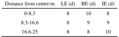
excavation face at the end of the first excavation intermission were examined (see Table 6 and

Fig.13). The unloading of the soil mass decreases the total stress of the soil beneath the excavation

face and induces negative excess pore-water pressures. The longer the exposure time of

excavation face was the more the negative excess pore-water pressure dissipated, therefore, the

decrease in effective stress beneath the excavation face was greater and the heave of pit base was

the exposure time under BE was the longest and therefore the heave of the base was the largest.

During IE the thick soil layer in the formation level centre was excavated later (as mentioned

above) and the negative excess pore-water pressures dissipated slowly. Therefore, the heave

deformations under IE were smaller than those under LE and BE.

Fig.12 Heave of formation level at the third excavation stage

Fig.13 Heave of formation level at the end of the first excavation intermission

Table 6 Exposure time of excavation face at the end of the first excavation intermission

Distance from centre/m LE (d) BE (d) IE (d)

0-8.3 8 10 8

8.3-16.6 8 9 9

16.6-25 8 8 10

0 2 4 6 8 10

0 3 6 9 12 15 18 21 24 27

He av e o f fo rm ati o n lev el (c m )

Distance from the formation level centre (m)

LE BE IE

0 2 4 6 8

0 3 6 9 12 15 18 21 24 27

He av e o f fo rm ati o n lev el (c m )

Distance from the formation level centre (m)

4.4 Pore-water pressure of excavation

The flow of ground water depends on soil water potential and defined as the sum of excess

pore-water pressure, hydrostatic pressure and the gravity potential. In order to analyse the flow of

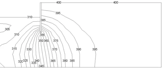
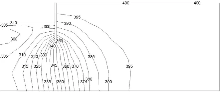
ground water inside and outside the excavation, under different excavation patterns, the contours

of the soil water potentials inside and outside the excavation at the x=0 section and at the third

excavation stage are shown in Figs.14-16, where the datum for the elevation head is at the bottom

boundary of model. It can be seen from Figs.14-16 that the soil water potentials outside the

excavation were all larger than the ones inside under the three excavation patterns at the third

excavation stage. Therefore, ground water flows into the excavation from the outside. For BE

ground water not only flows into the centre under excavation face but also observably flows into

the area near to the retaining structure. Since the soil close to the retaining wall was unloaded later

and the soil water potentials were also correspondingly less than the values under LE. Similarly,

the soil at the formation level centre under IE was excavated later and the dissipation of the soil

water potential at the centre was slow. Therefore, the ground water was more apt at flowing into

the excavation at the formation level centre than during LE.

Fig.15 Distribution of the soil water potentials under BE (unit: kPa)

Fig.16 Distribution of the soil water potentials under IE (unit: kPa)

Figs.17-19 show the contours of the excess pore-water pressures inside and outside the

excavation under the three patterns at the x=0 section and at the third excavation stage. It can be

seen from Figs.17-19 that at the third excavation stage the horizontal distribution range of the

negative excess pore-water pressures beneath excavation face under LE were the smallest. The

values under BE were the largest and the values under IE were between these two. However, the

vertical distribution range of the negative excess-pore water pressures beneath excavation face

under IE was the largest and the value under LE was the least. The comparison among the values

of negative excess pore-water pressure under different excavation patterns shows that the

Fig.17 Distribution of excess pore-water pressures under LE (unit: kPa)

Fig.18 Distribution of excess pore-water pressures under BE (unit: kPa)

Fig.19 Distribution of excess pore-water pressures under IE (unit: kPa)

The distribution difference of excess pore-water pressure is related to the unloading process

of the three excavation patterns. The unloading process of LE was uniform and the exposure time

of the whole excavation face was kept the same. This was favourable to the uniform dissipation of

unloading above the excavation face was non-uniform. The unloading under BE was from the

formation level centre to the retaining wall and it was just contrary under IE which is unfavourable

for the dissipation of the excess pore-water pressures. The negative excess pore-water pressures

under BE and IE dissipated slower and their areas were larger. In the process of BE larger negative

excess pore-water pressures were generated in the nearby retaining structure than the values under

LE as the result of the later unloading nearby retaining structure under BE. Moreover, the

process of IE was contrary to the one of BE and so its negative excess pore-water pressures at the

formation level centre were larger than the LE values.

5. Conclusions

3D effective stress analysis of an excavation under Layered, Basin and Island Excavation

processes was performed and reported in this work. This has led to the following conclusions:

(1) The soil around retaining wall was unloaded later under BE which decreased the exposure

time of the retaining structure and induced small horizontal displacements. It is, therefore,

favourable when controlling the deformation of a retaining wall. The soil at the formation level

centre was unloaded later under IE which decreased the exposure time of excavation face and

caused small heave of base and can be considered favourable when controlling any heave

deformation of the formation level.

(2) The settlement of the soil near the retaining wall was related to the wall deflection;

however, the settlement of soil at a reasonable distance from the wall was related to the dissipation

of negative excess pore-water pressure. For example the greater the negative excess pore-water

pressure was then the greater the effective stress of soil was and resulting in larger soil settlement.

were both very similar under the three excavation patterns. Since the order of unloading inside the

excavation was different then the scope of the negative excess pore-water pressure was larger (at

the excavation face) for the soil which was unloaded last.

In this work only the excavation patterns were focused on, however, excavation is an

over-consolidation problem due to unloading. Therefore, over-consolidation problem should be

considered when choosing a constitutive model of soil in future investigations.

References

[1] Hsieh P.G., Ou C.Y., 1998. Shape of ground surface settlement profiles caused by excavation. Canadian

Geotechnical Journal, 35: 1004-1017.

[2] Ou, C.Y., Liao, J.T., Cheng, W.L., 2000. Building response and ground movements induced by a deep

excavation. Geotechnique, 50(3): 209-220.

[3] Hsieh P.G., Ou C.Y., Liu H.T., 2008. Basal heave analysis of excavations with consideration of anisotropic

undrained strength of clay. Canadian Geotechnical Journal, 45: 788-799.

[4] Do T.N., Ou C.Y., Lim A., 2013. Evaluation of factors of safety against basal heave for deep excavations in

soft clay using the finite-element method. Journal of Geotechnical and geoenvironmental engineering,

139(12): 2125-2135.

[5] Hsieh P.G., Ou C.Y., Shih C., 2012. A simplified plane strain analysis of lateral wall deflection for

excavations with cross walls. Canadian Geotechnical Journal, 49:1134-1146.

[6] Hsieh P.G., Ou C.Y., Lin Y.L., 2013. Three-dimensional numerical analysis of deep excavations with cross

walls, Acta Geotechnica, 8:33-48.

[7] Ou C.Y., Hsieh P.G., Lin Y.L., 2013. A parametric study of wall deflections in deep excavations with the

[8] Wu S.H., Ching J.Y., Ou C.Y., 2013. Predicting wall displacements for excavations with cross walls in soft

clay. Journal of Geotechnical and Geoenvironmental Engineering, 139(6):914-927.

[9] Zdravkovic, L., Potts, D.M., St John, H.D,. 2005. Modelling of a 3D excavation in finite element analysis.

Geotechnique, 55(7):497-513.

[10] Kung G.T.C., Hsiao E.C.L., Juang C.H., 2007a. Evaluation of a simplified small-strain soil model for

analysis of excavation-induced movements. Canadian Geotechnical Journal, 44:726-736.

[11] Kung G. T. C., Juang C. H., Hsiao E. C. L., Hashash Y. M. A., 2007b. Simplified model for wall deflection

and ground-surface settlement caused by braced excavation in clays. Journal of Geotechnical and

Geoenvironmental Engineering, 133(6):731-747.

[12] Finno R.J., Blackburn J.T., Roboski J.F., 2007. Three-dimensional effects for supported excavations in clay.

Journal of Geotechnical and Geoenvironmental Engineering, 133(1):30-36.

[13] Osaimi A.E., Clough G.W., 1979. Pore-pressure dissipation during excavation. Journal of Geotechnical

Engineering, ASCE, 105(4): 481-498.

[14] Benmebarek, N., Benmebarek, S., Kastner, R., Soubra, A.H., 2006. Passive and active earth pressures in the

presence of groundwater flow. Geotechnique, 56(3):149-158.

[15] Li Y.Q., Zhou J., Xie K.H., 2008. Environmental effects induced by excavation. Journal of Zhejiang

University SCIENCE A, 9(1):50-57.

[16] Borges J.L., Guerra G.T., 2014. Cylindrical excavations in clayey soils retained by jet grout walls: Numerical

analysis and parametric study considering the influence of consolidation. Computers and Geotechnics,

55:42-56.

[17] Tan Y., Wang D., 2013a. Characteristics of a large-scale deep foundation pit excavated by the central-island

Geotechnical and Geoenvironmental Engineering, 139(11):1875-1893.

[18] Tan Y, Wang D., 2013b. Characteristics of a large-scale deep foundation pit excavated by the central-island

technique in Shanghai soft clay. II: Top-down construction of the peripheral rectangular pit. Journal of

Geotechnical and Geoenvironmental Engineering, 139(11):1894-1910.

[19] Potts D.M., Zdravkovic L., 1999. Finite element analysis in geotechnical engineering: Theory. Thomas

Telford Limited, London.

[20] Xie K.H., Zhou J., 2002. Theory and application of finite element analysis in geotechnical engineering.

Science Press, Beijing (in Chinese).

[21]Duncan, J.M., Chang, C.Y., 1970. Nonlinear analysis of stress and strain in soils. Journal of the Soil

Mechanics and Foundations Division, ASCE, 96(SM5), 1629-1653.

[22] Kulhawy, F.H., Duncan, J.M., 1972. Stresses and movements in Oroville Dam. Journal of the Soil

Mechanics and Foundations Division, ASCE, 98(SM7), 653-655.

[23] Ou C.Y., Wu T.S., Hsieh H.S., 1996. Analysis of deep excavation with column type of ground improvement

in soft clay. Journal Geotechnical Engineering, ASCE, 122(9):709-16.

[24] Liao H.J., 2009. Numerical analysis in geotechnical engineering (2nd _{Editon). Beijing: China Machine Press.}

[25] Yin Z.Z., Zhu H., Xu G.H., 1995. A study of deformation in the interface between soil and concrete.

Computers and Geotechnics, 17(1):75-92.

[26] Wang G.G., 1994. Theoretical Study on Large Strain of Deep Excavation. Ph.D Thesis, Tongji University,