Gradient-based Subspace Phase Correlation for Fast and Effective Image
Align-ment
Jinchang Ren, Theodore Vlachos, Yi Zhang, Jiangbin Zheng, Jianmin Jiang
PII:
S1047-3203(14)00116-3
DOI:
http://dx.doi.org/10.1016/j.jvcir.2014.07.001
Reference:
YJVCI 1396
To appear in:
J. Vis. Commun. Image R.
Received Date:
20 September 2013
Please cite this article as: J. Ren, T. Vlachos, Y. Zhang, J. Zheng, J. Jiang, Gradient-based Subspace Phase
Correlation for Fast and Effective Image Alignment,
J. Vis. Commun. Image R.
(2014), doi:
http://dx.doi.org/
10.1016/j.jvcir.2014.07.001
Gradient-based Subspace Phase Correlation
for Fast and Effective Image Alignment
Jinchang Ren
1, Theodore Vlachos
2, Yi Zhang
3, Jiangbin Zheng
4, Jianmin Jiang
5[email protected] [email protected] [email protected] [email protected] [email protected]
1
Centre for excellence in Signal and Image Processing, University of Strathclyde, Glasgow, U.K. 2
Department of Audiovisual Arts, Ionian University, Corfu, Greece. 3
School of Computer Software, Tianjin University, China 4
School of Computer Software and Microelectronics, Northwestern Polytechnical University, Xi’an, China 5
School of Computer Science and Software Engineering, Shenzhen University, Shenzhen, China
Abstract— Phase correlation is a well-established frequency domain method to estimate rigid 2-D translational motion between pairs
of images. However, it suffers from interference terms such as noise and non-overlapped regions. In this paper, a novel variant of the
phase correlation approach is proposed, in which 2-D translation is estimated by projection-based subspace phase correlation (SPC).
Conventional wisdom has suggested that such an approach can only amount to a compromise solution between accuracy and efficiency.
In this work, however, we prove that the original SPC and the further introduced gradient-based SPC can provide robust solution to
zero-mean and non-zero-mean noise, and the latter is also used to model the interference term of non-overlapped regions.
Comprehensive results from synthetic data and MRI images have fully validated our methodology. Due to its substantially lower
computational complexity, the proposed method offers additional advantages in terms of efficiency and can lend itself to very fast
implementations for a wide range of applications where speed is at a premium.
Keywords— Image registration, sub-pixel alignment, phase correlation, interference terms, subspace projection, Fourier transform.
Corresponding Author:
Dr Jinchang Ren
Dept. of Electronic and Electrical Engineering University of Strathclyde
204 George Street Glasgow, G11XW United Kingdom
Tel. +44-141-5482384
I. INTRODUCTION
Registration of images plays a crucial role in the analysis of multi-dimensional visual data in the digital domain, where at least two
images captured under different circumstances, such as from different sensors or at different times, need to be aligned for
consistent measurement and processing. This can benefit a wide range of applications, including remote sensing [1-2], motion
detection [3], image mosaicking [4, 36, 37], object recognition [5], medical imaging [6] and super-resolution for data visualization
[7] as well as surveillance and video compression [7, 8]. As a consequence the literature is enormous and any attempt to provide an
account of it would be out of the context of this paper. Apart from a comprehensive survey in [8], some more recent papers can be
found in [9-12], though they mainly focus on particular topics such as deformable medical image registration [9], remote sensing
image registration [10], evolutionary image registration methods for 3D modeling [11] and 2D/3D registration methods for
image-guided interventions [12].
Among many approaches proposed, phase correlation is a well-known technique for image registration [8][14], and has been
successfully used in many applications such as object recognition [13] and motion estimation [15][16]. Further applications
include verification in video shot detection [17] and motion extraction for video summarization and retrieval [18] [19]. The
baseline method utilizes the Fourier shift theorem, according to which shifts in the spatial domain correspond to linear phase
changes in the frequency domain. Phase correlation is then further extended to estimate changes of rotation and scale using the
Fourier-Mellin transform and the so-called pseudo-polar Fourier transform [20], [21]. However, estimation of shifts between
images with high accuracy remains a fundamental problem, in which potential exists for further research and improvement in terms
of sub-pixel registration [22], [23], video frame alignment [24] and blur-invariant registration [25].
Although pixel-level registration is adequate for some applications, higher accuracy sub-pixel registration is generally beneficial
to most applications [26], [27]. The need for sub-pixel registration arises from the simple fact that actual displacements between
images are oblivious to the discrete grid employed at the image acquisition stage. Additionally, in other applications such as
magnetic resonance imaging (MRI), data are usually sampled of non-integer offsets in the spatial Fourier domain before
reconstruction and sub-pixel registration by phase correlation is a natural approach in such a context. Detailed comparison of
several sub-pixel schemes can be found in [28].
Typically, 2-D Fourier transform is utilized by existing phase correlation approaches in estimating shifts between images. Its
complexity under fast implementation, however, still remains an issue for many applications, where massive amount of data are
involved. In addition, 2-D approaches perform less robustly, especially in estimating sub-pixels shifts in the presence of noisy data.
To this end, a more accurate and robust solution of sub-pixel accuracy is desirable, which forms the motivation of the work
The main contributions are highlighted as follows. Firstly, we derive a fast solution using projection-based subspace phase
correlation to estimate 2-D shifts in images, which is shown more robust to zero-mean noise than existing conventional approaches
using 2-D phase correlation. Secondly, gradient based subspace phase correlation is proposed to deal with non-overlapped regions
between the images under registration. These regions are taken as non-zero-mean noise in projected signals and it is proved that
they have less influence using the proposed scheme than otherwise. In addition, we also demonstrate that the proposed method will
yield higher peak than its 2-D counterpart.
The remaining part of this paper is organised as follows. Section 2 contains introductory concepts related to the phase correlation
approach and problem formulation. In Section 3, subspace phase correlation and its gradient based variant are presented and their
robustness is also demonstrated. Experimental results are given in Section 4 using synthetic data and MRI image data.
Comparisons with existing techniques are also provided to confirm the superiority against proposed techniques. Finally, brief
conclusions are drawn in Section 5.
II.PROBLEM FORMULATION
The baseline method of phase correlation is based on the Fourier shift theorem, which states that a shift in spatial domain will
lead to linear phase differences in Fourier domain. Let
r
(
x
,
y
)
andg
(
x
,
y
)
be two images satisfying)
)
(
,
)
((
)
,
(
x
y
g
x
x
0M
y
y
0N
r
=
−
⊕
−
⊕
in which the images areM
×
N
in size and⊕
refers to the modulo operator.Accordingly, the Fourier transforms
R
(
u
,
v
)
andG
(
u
,
v
)
of the images should satisfy) / / (
2 0 0
)
,
(
)
,
(
u
v
G
u
v
e
j ux M vy NR
=
− π + (1)Then, the phase difference can be obtained using the normalized cross-power spectrum as given below
) / / ( 2 *
*
0 0
)
,
(
)
,
(
)
,
(
)
,
(
)
,
(
e
j ux M vy Nv
u
G
v
u
G
v
u
G
v
u
R
v
u
P
=
=
− π + (2)where * is the complex conjugate,
j
=
−
1
, andP
(
u
,
v
)
is referred to as the cross power spectrum of the two images.If we apply the inverse Fourier transform
ℑ
−1 toP
(
u
,
v
)
, a phase correlation surface (PCS)p
(
x
,
y
)
can be obtained asfollows, which is essentially a Dirac function centered at
(
x
0,
y
0)
.(
(
,
)
)
(
,
)
)
,
(
0 01
y
y
x
x
v
u
P
y
x
p
=
ℑ
−=
δ
−
−
(3)If the two images under consideration are not perfect replicas of each other hence the surface is noisy due to interference terms
such as noise and non-overlapped regions. The latter will cause inconsistency due to the fact that the real shift is not a strict mod
recovered below, though the peak value can be less than unity as expected.
|
)
,
(
|
max
arg
)
,
(
, 00
y
p
x
y
x
y x
=
(4)Due to sub-pixel shifts, the peak value can also be substantially degraded since the peak energy can be distributed to several
adjacent neighbouring peaks [22]. Peak height is an indication of confidence to the estimate obtained especially in the presence of
the interference terms mentioned above. To enhance the peak identification accuracy in these cases pre-processing in the shape of
windowing or filtering is often considered. In our paper, however, such pre-processing measures have not been considered in order
to obtain cleaner and more straight-forward comparisons with competing methods i.e. comparisons which are not conditional upon
using a specific pre- or post- processing regime. Nevertheless, results using spatial windowing from conventional approaches are
also presented for evaluation purposes as discussed in Section 4.1.
Let
n
(
x
,
y
)
denote the effect of the interference terms, then the original two images satisfy)
,
(
)
)
(
,
)
((
)
,
(
x
y
g
x
x
0M
y
y
0N
n
x
y
r
=
−
⊕
−
⊕
+
(5)Let
C
rg(
x
d,
y
d)
=
E
[
r
(
x
,
y
)
g
(
x
+
x
d,
y
+
y
d)]
be the correlation function between two functionsr
andg
, whereE
refers to the mathematical expectation, the corresponding cross-power spectrum becomes [30]
)
,
(
/
)
,
(
)
,
(
)
,
(
)
,
(
)]
,
(
)
,
(
[
)]
,
(
[
)]
,
(
[
)]
,
(
[
)]
,
(
[
)]
,
(
[
)
,
(
) / / ( 2 * * ) / / ( 2 0 0 0 0 0 0v
u
G
v
u
N
e
v
u
G
v
u
G
v
u
G
v
u
N
e
v
u
G
y
x
C
y
x
C
y
y
x
x
C
y
x
C
y
x
C
v
u
P
N vy M ux j N vy M ux j d d gg d d ng d d gg d d gg d d rg n+
=
+
=
ℑ
ℑ
+
+
+
ℑ
=
ℑ
ℑ
=
+ − + − π π (6)As can be seen,
P
n(
u
,
v
)
is no longer a simple phase difference and it will approachP
(
u
,
v
)
only if we have0
)
,
(
/
)
,
(
u
v
G
u
v
→
N
, i.e. under a high signal to noise ratio (SNR). However, this requirement cannot be always satisfied,especially when there are non-overlapped regions between images. As a result, we have proposed the projection-based subspace
phase correlation to address this difficulty. Although the concepts of subspace and projection are not new in phase correlation, the
essence of our proposed algorithm still is original, considering the fact that most existing work either needs 2-D phase correlation
to enable subspace identification of displacement [15, 29] or shows lack of robustness [30]. In [15], based on the fact that the
noise-free model for the phase correlation matrix is a rank one matrix, a subspace extension is proposed to identify subpixel shifts
However, the phase correlation matrix needs still be generated through 2D phase correlation. For the phase correlation function
obtained from 2D Fourier transform, a masking operator is proposed in [29] to generate a projected one whilst rejecting
components that are unrelated to the estimated shifts. Then, Hoge’s approach [15] is applied to the so-called projected matrix to
determine subpixel shifts for improved accuracy. In [30], projection based subspace phase correlation is used for pixel-level image
registration. A windowing function is applied to the raw data before registration to avoid the failure of the approach. Without image
gradient, this approach can only deal with small displacements. On the contrary, our proposed algorithm uses only 1-D phase
correlation to estimate 2-D offsets in a robust way as explained in the next section. As demonstrated in (6), the results from 2-D
phase correlation suffer from the interference terms while we will show not only the efficiency but also the robustness of our
subspace phase correlation.
III. COPING WITH INTERFERENCE TERMS USING SUBSPACE PHASE CORRELATION
In this section, firstly subspace phase correlation is derived and proved to be robust to zero-mean interference terms. Secondly,
gradient based subspace phase correlation is further proposed to deal with non-zero-mean interference terms. Our method is shown
to yield higher levels of accuracy and robustness and is not liable to the simple trade-off between accuracy and efficiency as
reported in [30], [31], [32]. In [30], without image gradient and a subpixel scheme, projection-based subspace phase correlation can
only deal with pixel-level small displacements between images. In [31], integral projections are used for block motion estimation
within video frames. Rather than using phase correlation, the mean absolute error is used to determine the pixel-level motion
vector. Although the computational cost is low, the overall accuracy is limited. In [32], projection based phase correlation is used to
extract motion fields between image pairs within image sequences. It is found that subspace phase correlation reaches tradeoffs of
computational efficiency and accuracy.
A.Subspace Phase Correlation
Let
r
x(
x
)
andg
x(
x
)
denote respectively subspace projections ofr
(
x
,
y
)
andg
(
x
,
y
)
ontox
axis, and let their corresponding 1-D Fourier transforms be denoted asR
x(
u
)
andG
x(
u
)
,))
(
(
)
(
,
)
,
(
)
(
x
r
x
y
R
u
r
x
r
x xy
x
=
∑
=
ℑ
(7)))
(
(
)
(
,
)
,
(
)
(
x
g
x
y
G
u
g
x
g
x xy
x
=
∑
=
ℑ
(8))
0
,
(
)
,
(
)
,
(
)
(
) / 0 / ( 2 / 2u
R
e
y
x
r
e
y
x
r
u
R
x y N y M ux j x y M ux j x=
=
=
∑∑
∑∑
⋅ + − − π π (9))
0
,
(
)
,
(
)
(
u
g
x
y
e
2 /G
u
G
x y
M ux j
x
=
∑∑
=
− π
(10)
where
R
(
u
,
v
)
andG
(
u
,
v
)
are the 2-D Fourier transforms ofr
(
x
,
y
)
andg
(
x
,
y
)
, respectively.If there are no interference terms, from (1) we have
M ux j
e
u
G
u
R
(
,
0
)
=
(
,
0
)
− 2π 0/(11)
If we substitute (9) and (10) in (11), it derives
M ux j x x
u
G
u
e
R
(
)
=
(
)
− 2π 0/(12)
which clearly shows that
R
x(
u
)
andG
x(
u
)
are related by a phase difference that originates fromr
x(
x
)
=
g
x(
x
−
x
0)
.As a result, 1-D phase correlation can be used to estimate the shift in the
x
direction as shown below:M ux j x x x x x
e
u
G
u
R
u
G
u
R
u
P
2 /* * 0
)
(
)
(
)
(
)
(
)
(
=
=
− π (13)(
(
)
)
(
)
)
(
x
1P
u
x
x
0p
x=
ℑ
− x=
δ
−
(14)Similarly,
y
0 can also be estimated from 1-D phase correlation using the 1-D Fourier transform of projected signal toy
direction as follows:
N vy j y y y y y
e
v
G
v
R
v
G
v
R
v
P
2 /* * 0
)
(
)
(
)
(
)
(
)
(
=
=
− π (15)( )
(
)
(
)
)
(
y
1P
v
y
y
0p
y=
ℑ
y=
−
−
δ
(16)
where
R
y(
v
)
andG
y(
v
)
are respectively 1-D Fourier transforms of the projected signals,r
(
x
,
y
)
andg
(
x
,
y
)
, onto they
axis.B. Dealing with the Interference Terms
Considering the interference terms, we no longer have
r
x(
x
)
=
g
x(
x
−
x
0)
. Instead,r
x(
x
)
can be derived below))
,
(
(
)
(
)
(
x
g
x
x
0N
E
n
x
y
r
x=
x−
+
⋅
(17)∑
− ==
1 0)
,
(
1
))
,
(
(
N yy
x
n
N
y
x
n
where
E
(
n
(
x
,
y
))
refers to the average value (mean) of all contributing samples ofn
(
x
,
y
)
.If the number
N
is large enough and the effect of the interference terms exhibits as zero-mean noise, not necessarily Gaussian,we have
E
(
n
(
x
,
y
))
=
0
hence we still have simple spatial shifts between projected signals which will lead to linear phase difference as given in (13) and (15). This indicates that the projected signal virtually eliminates the influence of the random noisecomponent which renders the subspace phase correlation more robust in relation to conventional 2-D phase correlation.
Regarding non-zero-mean effect of the interference terms, gradient-based information is considered. Let
r
x(
x
)
be the horizontal projection ofr
(
x
,
y
)
and its gradient signalr
x(1)(
x
)
=
r
x(
x
+
1
)
−
r
x(
x
)
can be derived as follows:∑
∑
∑
∑
− = − = − = − =−
⊕
+
=
+
−
=
−
⊕
+
=
1 0 1 0 ) 1 ( ) 1 ( 0 ) 1 ( 1 0 1 0 ) 1 ()
,
(
)
,
)
1
((
)
(
)
(
)
(
)
,
(
)
,
)
1
((
)
(
N y N y x x x N y N y xy
x
n
y
M
x
n
x
n
x
n
x
x
g
y
x
r
y
M
x
r
x
r
(19)where
g
(x1)(
x
)
and(
)
) 1 (
x
n
x are respectively the local gradient of the horizontal projection ofg
(
x
,
y
)
andn
(
x
,
y
)
. If we take the effect ofn
(
x
,
y
)
as non-zero-mean noise, when N is large enough we can easily derive))
(
(
)
,
(
)
,
)
1
((
1 0 1 0x
n
E
N
y
x
n
y
M
x
n
x N y N y⋅
=
=
⊕
+
∑
∑
=− =− (20)where
=
−∑
y x
x
N
n
x
y
n
E
(
(
))
1(
,
)
.In other words, we have
n
(1)(
x
)
=
0
x which will lead to a simple spatial shifts between
(
)
) 1 (x
r
x and(
)
) 1
(
x
g
x . As a result, linearphase difference will be generated to estimate
x
0 using subspace phase correlation between the two gradient signals. Similarly, wecan prove that
(
)
(
0)
) 1 ( ) 1 (
y
y
g
y
r
y=
y−
and use it to estimate y0. This has clearly indicated that gradient based subspace phasecorrelation can help to overcome the effect of non-zero-mean noise; again it can be Gaussian or non-Gaussian.
Finally, the masking operator introduced in [26] is applied to the phase correlation surface, which is useful in improving both the
robustness and efficiency. The latter is achieved in fast identifying the corresponding peaks as only a small portion of the samples
are considered. The estimate of
x
0 and y0 then becomes)
(
max
arg
ˆ
0 2 /0
p
x
x
xw M x∈ ±
=
ˆ
arg
max
(
)
0 2 /
0
p
y
y
yh N y∈ ±
where
w
0=
M
/
16
andh
0=
N
/
16
. Accordingly, the rangex
∈
M
/
2
±
w
0 to determinex
ˆ
0 becomes]
16
9
,
16
7
[
M
M
x
∈
,where only one-eighth of the samples are remained for consideration. Similarly,
y
ˆ
0 is also determined by using only one-eighth ofthe samples. Further improvements may include spatial windowing for more robustness as suggested in [29].
C.Peak Height Analysis
If we take into account the expressions describing 2-D phase correlation (2)-(3) on the one hand and those describing the
subspace variant (13)-(16) on the other hand, we can easily establish that:
)
(
)
(
)
,
(
)
(
)
(
)
,
(
y
p
x
p
y
x
p
v
P
u
P
v
u
P
y x y x=
=
(22)Since all the PCS surfaces are upper bound to unity, i.e.
|
p
x(
x
)
|
≤
1
,|
p
y(
y
)
|
≤
1
and|
p
(
x
,
y
)
|
≤
1
, we have|
)
,
(
|
|
)
(
/
)
,
(
|
|
)
(
|
|
)
,
(
|
|
)
(
/
)
,
(
|
|
)
(
|
y
x
p
x
p
y
x
p
y
p
y
x
p
y
p
y
x
p
x
p
x y y x≥
=
≥
=
(23)The above is a simple illustration of the fact that subspace phase correlation tends to yield higher peaks than those obtained from
2-D phase correlation. The higher peak here is useful in accurately identifying the potential matching of linear phase difference,
especially under noisy situations. In real cases, the height of the side-peak depends on both the sub-pixel shifts and the interference
terms [22]. Consequently, the effectiveness of the peak height is further measured by the accuracy of the recovered sub-pixel shifts,
which are presented and discussed in the next section.
IV. RESULTS AND DISCUSSIONS
The performance of proposed method was determined by using both synthetic and real data. For synthetic data, sub-pixel shifts
of images are generated by down-sampling of the original images. As for real data, a set of MRI images of sub-pixel displacements
are employed.
Using ground truth (real shifts) as a reference, an error vector between a real shift and the corresponding estimate is obtained for
each method along the x and y directions. Let
δ
x andδ
y denote the corresponding error vectors, i.e. δx(i)=x(i)−xˆ(i) and) ( ˆ ) ( )
(i yi y i
y = −
δ , where x(i) and y(i) are the th
i real offsets, and xˆ(i) and yˆ(i) are their estimates. The mean squared error
(MSE) between the estimates and the ground truth, as defined in (24), is used as an overall measurement and this is consistent with
y
x
z
i
n
z
MSE
n i
z
(
)]
,
,
[
1
)
(
1
2
=
=
∑
=
δ
(24)
A.Synthetic Data
In Fig. 1, four original test images namely “airfield”, “Barbara”, “image043” and “pentagon” are shown. These are 8bpp images
and their sizes are 512×512 pixels. To obtain sub-pixel displacements, the same strategy used in [22] and [23] is applied to these
two original images, i.e. sub-pixel shifts are obtained by lowpass-filtering and down-sampling of a real high resolution. Since these
sub-pixel shifts may lead to non-overlapped contents in the image, gradient-based subspace phase correlation is employed to deal
with such cases.
Since the original images we obtained are of a given resolution, up-sampling is utilized to manually generate images of high
resolution before down-sampling is applied to yield images of sub-pixel shifts. The integer up-sampling and down-sampling
factors are not limited to power of two, which are determined by the demanded sub-pixel shifts as follows. If the sub-pixel part of
the offsets are 2/3 and 1/4 in x and
y
axes, the upsampling factors in horizontal and vertical directions are 3 and 4, respectively.Then, sub-pixel shifts are achieved by integer shifts of 2 and 1 pixels in upsampled image followed by downsampling. Please note
that the downsampled image is of the same size as the original one.
If an offset contains integer part, it can be easily implemented by shifting the down-sampled image in corresponding pixels.
Since such shifts may lead to non-overlapped pixels in images, normally these are treated as black pixels with intensity values of
zero. However, this will introduce sharp intensity changes along the black boundary and cause inaccurate image gradient in
subspace phase correlation. To address this problem, we simply ignore a wide boundary in gradients of projected signals by
assigning their values as zero before applying subspace phase correlation. Currently, the boundary is set as one-eighth of the image
dimension in two directions, respectively, as we suppose the shifts should not exceed such a range. It is found that this can not only
effectively solve the problem but also improve the efficiency as the cropped image contains one-fourth of zero samples.
To further reduce the artifacts caused by data resampling, Gaussian smoothing is applied to the upsampled image as low-pass
filtering. Since Gaussian filter is separable, two 1-D Gaussian filters are applied to x and
y
axis, respectively. The size of theGaussian kernel is decided as
2
l
−
1
wherel
is the up-sampling factor. Finally, the smoothed image is obtained via convolution of the upsampled image with the decided Gaussian kernel. It is worth noting that the Gaussian filter used here is a low-pass one, whichhas the potential to reduce aliasing effect towards robust image registration [7]. In addition, it is worth noting that the Gaussian
variance between 0.5 and 1.2 is found to produce relatively better results.
In our experiments, in total 13 shifts are used in both horizontal and vertical directions, which help to produce 169 shifted images
0
and 3/4 are used plus integer shifts varying from 0 to 6. These form a wide range of offsets in our experiments, and for each test
image the average registration error is determined over all 169 shifted versions as reported in Table I. In Table I, our results are
compared with those obtained from Stone [2], Hoge [15], Foroosh [22] and Tzimiropoulos [33]. Please note that only the
translational part of the approach in [33] was implemented for benchmarking as we only deal with image shifts. To further enable
consistent evaluations, the results from phase correlation with spatial windowing using the standard Blackman window are also
[image:11.612.66.535.252.402.2]presented in Table I.
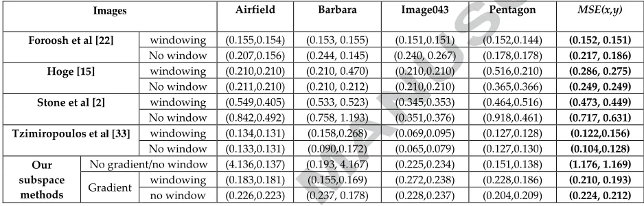
Table I. Table of results for shifts of the images in Fig. 1 using downsampling with or without windowing.
Images Airfield Barbara Image043 Pentagon MSE(x,y)
Foroosh et al [22] windowing (0.155,0.154) (0.153, 0.155) (0.151,0.151) (0.152,0.144) (0.152, 0.151)
No window (0.207,0.156) (0.244, 0.145) (0.240, 0.267) (0.178,0.178) (0.217, 0.186) Hoge [15] windowing (0.210,0.210) (0.210, 0.470) (0.210,0.210) (0.516,0.210) (0.286, 0.275)
No window (0.211,0.210) (0.210, 0.212) (0.210,0.210) (0.365,0.366) (0.249, 0.249) Stone et al [2] windowing (0.549,0.405) (0.533, 0.523) (0.345,0.353) (0.464,0.516) (0.473, 0.449)
No window (0.842,0.492) (0.758, 1.193) (0.351,0.376) (0.918,0.461) (0.717, 0.631) Tzimiropoulos et al [33] windowing (0.134,0.131) (0.158,0.268) (0.069,0.095) (0.127,0.128) (0.122,0.156)
No window (0.133,0.131) (0.090,0.172) (0.065,0.079) (0.127,0.130) (0.104,0.128) Our
subspace methods
No gradient/no window (4.136,0.137) (0.193, 4.167) (0.225,0.234) (0.151,0.138) (1.176, 1.169)
Gradient windowing (0.183,0.181) (0.155,0.169) (0.272,0.238) (0.228,0.186) (0.210, 0.193) no window (0.226,0.223) (0.237, 0.178) (0.228,0.237) (0.204,0.209) (0.224, 0.212)
To achieve sub-pixel accuracy, two 1-D Gaussian curves are fitted using the dominant peak
p
(
x
0,
y
0)
and two neighboring peaks whereC
m,n=
|
p
(
x
0+
m
,
y
0+
n
)
|
andm
,
n
∈
{
−
1
,
0
,
1
}
[24]. This is also applied to Tzimiropoulos’s approach [33] whensubpixel shifts are estimated. All four competing approaches use 2-D phase correlation are then compared against our proposed
gradient-based subspace phase correlation.
1 , 0 1 , 0 0
, 0
1 , 0 1
, 0
0 , 1 0 , 1 0
, 0
0 , 1 0
, 1
log
log
2
log
log
ˆ
log
log
2
log
log
ˆ
− −
− −
−
−
−
=
−
−
−
=
C
C
C
C
C
y
C
C
C
C
C
x
Gau Gau
(25)
As can be seen, the following observations can be made from Table 1. First, under 2D phase correlation, Stone’s approach [2]
yields worse results in terms of highest MSE errors, followed by results from Hoge [15], Foroosh [22] and Tzimiropoulos [33].
Second, spatial windowing provides noticeable improvements to the estimated results for Stone [2] and Foroosh [22], yet the
improvements on other approaches are limited. Third, for the proposed subspace phase correlation, image gradient has
1
Occasionally, both Hoge’s [15] and Stone’s [2] methods fail in estimating the corresponding shifts, no matter spatial windowing is
used or not. This is probably due to the SVD decomposition in [15] and least-squares estimate in [2] as these are extremely
sensitive to the change of image contents caused by downsampling. Finally, due to image gradient used with Gaussian fitting for
subpixel estimation, Tzimiropoulos’ approach [33] outperforms all others in this group of experiments. Considering subspace
phase correlation used in our approach, the results from ours are still quite satisfactory in comparison to those from Foroosh [22]
and Tzimiropoulos [33].
In addition, the results using subspace phase correlation without gradient are also shown in Table I for comparisons. Although it
may generate better results than those with gradient, see results for “image043” and “pentagon”, it fails for other images such as
wrong estimates for shifts in horizontal and vertical directions in “airfield” and “Barbara” images, respectively. Thanks to
gradient-based subspace phase correlation, this problem has been resolved towards accurate and reliable image registration.
B.Real MRI Data
The MRI data set used in our experiments is courtesy of W. S. Hoge and contains five MRI images of a grapefruit (size of
256×256 in 8-bit grey format) [15]. The true shifts between each pair of images are known and subsequently used as ground truth
for performance evaluation. The first MRI image is shown in Fig. 2, along with two other images obtained by manually adding
Gaussian noise. We compare our method against the techniques of Hoge [15], Foroosh et al [22], Balci and Foroosh [23], and
Tzimiropoulos’ approach [33] and tabulate the results in Table II, where the results in [23] are directly quoted.
Please note that the results in Table II are not the same as reported in our previous paper [34] due to different sub-pixel strategies
used. In [34], linear interpolation between the first two highest peaks is used for subpixel registration, where the integer offset is
remained if the heights of the two side peaks are within a given threshold. Apparently, the performance can be affected by the
selected threshold. In this paper, however, subpixel accuracy is achieved through fitting two 1-D Gaussian curves over the
dominant peak and the two side peaks, where no thresholding is needed. In addition, with similar results generated using a different
subpixel strategy, it shows the effectiveness of the approach is mainly due to the proposed subspace phase correlation.
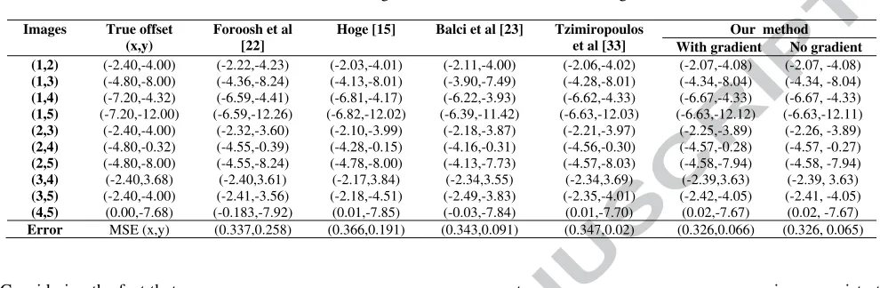
In Table II, the MSE measurements in x and y directions are given again for comparison purposes. It can be clearly seen that
the overall accuracy along they-axis is better than that along x-axis, which is possibly due to the difference in generating
displacements in different directions (see [15] for details). In x direction, our method yields the minimum error, followed by the
approaches from Foroosh [22], Balci [23], Tzimiropoulos [33] and Hoge [15]. In y direction, our method is slightly worse than
Tzimiropoulos [33] and generates the second minimum error, followed by [23], [15] and [22]. Overall, the proposed approach is
among the best in this group of experiments.
As there are no noise effects caused by non-overlapped regions in these test images, the advantage of gradient-based subspace
2
projected signals without the use of local gradient information. For synthetic data, this will normally lead to performance
compromise. However, for the MRI data the results are almost the same as those in Table II with local gradient applied, which
[image:13.612.57.552.152.314.2]shows that our approach can still estimate the corresponding displacements successfully.
Table II. Pair-wise registration results of the five MRI images.
Images True offset (x,y)
Foroosh et al [22]
Hoge [15] Balci et al [23] Tzimiropoulos et al [33]
Our method With gradient No gradient (1,2) (-2.40,-4.00) (-2.22,-4.23) (-2.03,-4.01) (-2.11,-4.00) (-2.06,-4.02) (-2.07,-4.08) (-2.07, -4.08)
(1,3) (-4.80,-8.00) (-4.36,-8.24) (-4.13,-8.01) (-3.90,-7.49) (-4.28,-8.01) (-4.34,-8.04) (-4.34, -8.04)
(1,4) (-7.20,-4.32) (-6.59,-4.41) (-6.81,-4.17) (-6.22,-3.93) (-6.62,-4.33) (-6.67,-4.33) (-6.67, -4.33)
(1,5) (-7.20,-12.00) (-6.59,-12.26) (-6.82,-12.02) (-6.39,-11.42) (-6.63,-12.03) (-6.63,-12.12) (-6.63,-12.11)
(2,3) (-2.40,-4.00) (-2.32,-3.60) (-2.10,-3.99) (-2.18,-3.87) (-2.21,-3.97) (-2.25,-3.89) (-2.26, -3.89)
(2,4) (-4.80,-0.32) (-4.55,-0.39) (-4.28,-0.15) (-4.16,-0.31) (-4.56,-0.30) (-4.57,-0.28) (-4.57, -0.27)
(2,5) (-4.80,-8.00) (-4.55,-8.24) (-4.78,-8.00) (-4.13,-7.73) (-4.57,-8.03) (-4.58,-7.94) (-4.58, -7.94)
(3,4) (-2.40,3.68) (-2.40,3.61) (-2.17,3.84) (-2.34,3.55) (-2.34,3.69) (-2.39,3.63) (-2.39, 3.63)
(3,5) (-2.40,-4.00) (-2.41,-3.56) (-2.18,-4.51) (-2.49,-3.83) (-2.35,-4.01) (-2.42,-4.05) (-2.41, -4.05)
(4,5) (0.00,-7.68) (-0.183,-7.92) (0.01,-7.85) (-0.03,-7.84) (0.01,-7.70) (0.02,-7.67) (0.02, -7.67)
Error MSE (x,y) (0.337,0.258) (0.366,0.191) (0.343,0.091) (0.347,0.02) (0.326,0.066) (0.326, 0.065)
Considering the fact that accurate image registration
error measures than expected ones as being pointed out in [15]. As a result, the relative error
RE
in [15] is also utilized forconsistent evaluation, which is defined using the Frobenius norm as
2 / 1 ,
2
]
[
/
)
,
,
(
)
,
,
,
(
∑
=
−
=
j i ij F
F F
a
A
A
y
x
B
MC
A
y
x
B
A
RE
(26)
where
(
x
,
y
)
is the estimated shift betweenA
andB
, andMC
denotes motion compensation in which linear interpolation isutilized for improved accuracy. It is worth noting that, due to the y-axis is defined up-side-down in images,
(
−
x
,
y
)
needs to beused for correct motion compensation of
B
. Finally, theRE
measures for the 10 image pairs in Table II are displayed in Fig. 3.Table III. Average relative error RE vs. registration methods for the ten pairs of images in Table II.
Method GT Foro [22] Hoge[15] Balci[23] Tzimiropoulos[33] Our RE 0.1158 0.1065 0.1127 0.1187 0.1031 0.1024
In Fig. 3, although the absolute values of the attained
RE
measures are different from those in [15] and [23], the curves arequite similar, especially the one using the “physical shifts”. As can be seen, indeed most of the estimates have less error than
knowledge of prescribed physical shifts, except the results for the last three image pairs. Again, the results of our method have
minimum relative errors, followed by the results from Tzimiropoulos [33], Foroosh [22], Hoge [15] and Balci [23]. This is
3
relative errors listed in Table III also validate the analysis above. It is worth noting that our proposed approach outperforms all
others in this group of experiments.
C.Robustness Analysis
To evaluate the robustness of our approach, synthetic zero-mean Gaussian noise is added to the test images. Before adding noise,
the intensity level of the original images is normalized within [0,1]. Then, zero-mean Gaussian noise is generated with its variance
changing linearly in eight levels within the interval [0.005,0.04], hence eight noisy samples are obtained for each of the five
original images. Two example images with additive noise are shown in Fig. 2. For the original image in Fig. 2, the noise level of its
8 noisy samples are further measured in terms of the signal to noise ratio (SNR), which are 29.2, 22.8, 18.9, 16.2, 14.0, 12.3, 10.9
and 9.5db, respectively.
Again, pair-wise registration is performed, thus totally 80 pairs of noisy images are used for 8 different noise levels (Gaussian
variance values). For each noise level, all the estimates from 10 pairs of images are measured using the MSE criterion. Hoge’s
method was found to fail in most of the noisy cases. Results obtained from our approach are compared with those from Foroosh et
al [22] as shown in Fig. 4. As can be seen, in general, Foroosh’s method generates higher MSE, though there are some exceptions
along the y-axis. Along the x-axis, subspace phase correlation usually yields consistently lower levels of MSE than the 2-D
approach.
The height of the most dominant peak can be considered as an indication of robustness. Here the height ratio between the main
peak and the second peak is not considered as the height of the latter depends on the sub-pixel shifts and other effects as mentioned
in Section 3. Fig. 5 shows the average height of the most dominant peak as a function of increasing Gaussian variance for 2-D
correlation and subspace correlation (along the x- and y- axes). With increasing Gaussian variance, the average height from 2-D or
subspace correlation decreases subsequently. However, it is obvious that subspace correlation generates much higher average
peaks than 2-D correlation, in accordance with our discussions in Section 3.3.
D.Computational Complexity
In both 2-D phase correlation and subspace correlation, the fast Fourier transform (FFT) is the main computational load. In some
approaches, additional processing is required such as windowing, partial differencing or even singular value decomposition [15]
and iterative optimization [23]. If the original images are of N×N, then the computing complexity of the FFT in 2-D and subspace
correlation is
Ο
(
N
2log
2N
)
and(
log
)
2
N
N
Ο
, respectively. Considering the projection needed in the proposed algorithm, thecomplexity of our proposed subspace phase correlation is not
N
times faster than conventional 2-D phase correlation. Furthercomparison of execution time using both 2-D phase correlation and subspace phase correlation is presented in Table IV, which is
4
Fig. 1 at size of 256×256 and 512×512, respectively. Again, it has fully demonstrated the efficiency of proposed approach. In
summary, our subspace scheme is of substantially lower complexity and consequently faster to implement. In addition, all the
components in our approach, including the FFT, subspace projection, local gradient and linear interpolation are suitable for
hardware implementation to further improve the efficiency.
Finally, it is worth noting that the complexity of Hoge [15] and Stone [2] is significant higher than those of Foroosh [22] and of
course our proposed approach. For registration of one image pair of 512×512 pixels, the relative computational complexity can be
compared as follows. If we take the complexity of subspace phase correlation as 1, then the complexity for 2-D phase correlation
[22], Hoge [15] and Stone [2] are 16.7, 73.8 and 1574.3, respectively, which correspondingly refer to 0.047s, 0.78s, 3.5s, and 73.8s.
This again shows the superiority of the proposed approach.
Table IV. Comparison of execution time in milliseconds for 2-D and sub-space phase correlation at different image sizes.
Method Size
2-D phase correlation Subspace correlation Windowing No window Gradient No gradient
256×256 184.4 168.6 12.5 12.5
512×512 780.5 718.1 46.9 46.8
V.CONCLUSIONS
Analysis of a novel extension to the phase correlation image registration approach has been described, where the presented
gradient-based subspace phase correlation was proved to be not only more efficient but also more effective and robust than
conventional 2-D phase correlation. The robustness to both zero-mean noise and non-zero-mean noise has been proved
theoretically and empirically. In addition, it is found that the masking operator is very useful in accurate and fast identification of
the dominant peak on the correlation surface. Finally, the fact that the proposed algorithm is suitable for hardware implementation
makes it a good candidate for a wide variety of applications like online registration and camera stabilization, although in an
unlikely happened special case it may fail when the projected signal becomes flat. Future investigations include extension of the
proposed method in an iterative scheme to further improve the accuracy and robustness as well as to apply the method for the
registration of video images. Rather than others in dealing with specific noise [35], the proposed gradient-based subspace phase
correlation shows great potential in coping with various interference terms for robust image registration.
ACKNOWLEDGMENT
The authors would like to thank Dr. W. S. Hoge for kindly providing the MRI data set and the Matlab codes for his algorithm,
which enabled some of the comparisons contained in this paper. Thanks are also due to Dr. V. Argyriou, University of Kingston for
5
REFERENCES
[1] Y. Bentoutou, N. Taleb, K. Kpalma, and J. Ronbin, “An Automatic Image Registration for Applications in Remote Sensing,” IEEE Trans. Geosci. Remote
Sens., vol. 43, no. 9, pp. 2127-2137, 2005.
[2] H. S. Stone, M. Orchard, E.-C. Chang, and S. Martucci, “A Fast Direct Fourier-based Algorithm for Sub-pixel Registration of Images,” IEEE Trans. Geosci.
Remote Sens., vol. 39, no. 10, pp. 2235–2243, 2001.
[3] E. De Castro and C. Morandi, “Registration of Translated and Rotated Images Using Finite Fourier Transforms,” IEEE Trans. PAMI, vol. 9, no. 5, pp.
700-703, 1987.
[4] S. Zokai and G. Wolberg, “Image Registration Using Log-polar Mapping for Recovery of Large-scale Similarity and Projective Transformations,” IEEE
Trans. Image. Proc., vol. 14, no. 10, pp. 1422-1434, 2005.
[5] G. Caner, A. M. Tekalp, G. Sharma, and W. Heinzelman, “Local Image Registration by Adaptive Filtering,” IEEE Trans. Image. Proc., vol. 15, no. 10, pp.
3053-3065, 2006.
[6] R. J. Althof, M. G. J. Wind, and J. T. Dobbins, “A Rapid and Automatic Image Registration Algorithm with Sub-pixel Accuracy,” IEEE Trans. Medical
Imaging, vol. 16, no. 3, pp. 308-316, 1997.
[7] P. Vandewalle, S. Susstrunk, and M. Vetterli, “A Frequency Domain Approach to Registration of Aliased Images with Application to Super-resolution,”
EURASIP J. Applied Signal processing, DOI 10.1155/ASP/2006/71459, pp. 1-14, 2006.
[8] B. Zitova and J. Flusser, “Image Registration Methods, a Survey,” Image and Vision Comput., vol. 21, no. 11, pp. 977-1000, 2003.
[9] A. Sotiras, C. Davatzikos and N. Paragios, Deformable medical image registration: a survey, IEEE Trans. Medical Imaging, vol. 32, no. 7, pp. 1153-1190,
2013
[10] S. Dawn, V. Saxena and B. Sharma, Remote Sensing Image registration techniques: a survey, Lecture Notes in Computer Science, vol. 6134, pp. 103-112,
2010
[11] J. Santamaria, O. Cordon, S. Damas, A comparative study of state-of-the-art evolutionary image registration methods for 3D modeling, Computer Vision and
Image Understanding, vol. 115, no. 9, pp. 1340-1354, 2011
[12] P. Markelj, D. Tomazevic,, B. Likar, F. Pernus, A review of 2D/3D registration methods for image-guided interventions, Medical Image Analysis, vol. 16, no.
3, pp. 642-661, 2012
[13] Q. Chen, M. Defrise, and F. Deconinck, “Symmetric Phase-only Matched Filtering of Fourier-Mellin Transforms for Image Registration and Recognition”.
IEEE Trans. PAMI, vol. 16, no. 12, pp. 1156-1168, 1994.
[14] D. Robinson and P. Milanfar, “Fundamental Performance Limits in Image Registration,” IEEE Trans. Image Proc., vol. 13, no. 9, pp. 1185-1199, 2004.
[15] W. S. Hoge, “Subspace Identification Extension to the Phase Correlation Method”. IEEE Trans. Medical Imaging, vol. 22, no. 2, pp.277-280, 2003.
[16] S. Erturk, “Digital Image Stabilization with Subimage Phase Correlation Based Global Motion Estimation,” IEEE Trans. Consumer Electron., vol. 49, no. 4,
pp. 1320-1325, 2003.
[17] J. Ren, J. Jiang and J. Chen, “Shot boundary detection in MPEG videos using local and global indicators,” IEEE Trans. Circuits and Systems for Video
Technology, vol. 19, no. 8, pp. 1234-1238, 2009
[18] J. Ren and J. Jiang, “Hierarchical modeling and adaptive clustering for real-time summarization of rush videos,” IEEE Trans. Multimedia, vol. 11, no. 5, pp.
906-917, 2009
[19] J. Jiang, et al, “LIVE: an integrated production and feedback system for intelligent and interactive TV Broadcasting,” IEEE Trans. Broadcasting, vol. 57, no.
6
[20] Y. Keller, Y. Shkolnisky and A. Averbuch, “The Angular Difference Function and Its Application to Image Registration,” IEEE Trans. PAMI, vol. 27, no. 6,
pp. 969-976, 2005.
[21] B. S. Reddy and B. N. Chatterji, “An FFT-based Technique for Translation, Rotation, and Scale-invariant Image Registration,” IEEE Trans. Image Proc., vol.
5, no. 8, pp. 1266–1271, 1996.
[22] H. Foroosh, J. B. Zerubia, and M. Berthod, “Extension of Phase Correlation to Sub-pixel Registration,” IEEE Trans. Image Proc., vol. 11, no. 3, pp. 188–200,
2002.
[23] M. Balci and H. Foroosh, “Sub-pixel Estimation of Shifts Directly in the Fourier Domain,” IEEE Trans. Image Proc., vol. 15, no. 7, pp. 1965-1972, 2006.
[24] I. E. Abdou, “Practical Approach to the Registration of Multiple Frames of Video Images,” Proc. SPIE, vol. 3653, pp. 371-382, 1999.
[25] V. Ojansivu and J. Heikkila, “Image Registration Using Blur-Invariant Phase Correlation,” IEEE Signal Proc. Letters, vol. 14, no. 7, pp. 449-452, 2007
[26] H. Shekarforoush, M. Berthod, and J. Zerubia, “Subpixel Image Registration by Estimating the Polyphase Decomposition of Cross Power Spectrum,” Proc.
CVPR, pp. 532-537, 1996.
[27] F. Humblot, B. Collin, and A. Mohammad-Djafari, “Evaluation and Practical Issues of Subpixel Image Registration using Phase Correlation Methods,” Proc.
PSIP (Physics in Signal and Image Proc.), Toulouse, France, 2005.
[28] J. Ren, J. Jiang and T. Vlachos, “High-accuracy sub-pixel motion estimation from noisy images in Fourier domain,” IEEE Trans. Image Processing, vol. 19,
no. 5, pp. 1379-1384, 2010
[29] Y. Keller and A. Averbuch, “A Projection-based Extension to Phase Correlation Image Alignment,” Signal Proc., vol. 87, no. 1, pp. 124-133, 2007.
[30] S. Alliney and C. Morandi, “Digital Image Registration Using Projections,” IEEE Trans. PAMI, vol. 8, no. 2, pp. 222-233, 1986
[31] K. Sauer and B. Schwartz, “Efficient Block Motion Estimation Using Integral Projections,” IEEE Trans. Circuits Syst. Video Technol., vol. 6, no. 5, pp.
513-518, 1996.
[32] D. Robinson and P. Milanfar, “Efficiency and Accuracy Tradeoffs in Using Projections for Motion Estimation,” Proc. 35th Asilomar Conf. Signals, Systems,
and Computers, pp. 1425-1437, 2001
[33] G. Tzimiropoulos, V. Argyriou, S. Zafeiriou, and T. Stathaki, “Robust FFT-based Scale-Invariant Image Registration with Image Gradients,” IEEE Trans.
PAMI, vol. 32, no. 10, pp. 1899-1906, Oct. 2010.
[34] J. Ren, T. Vlachos and J. Jiang, “Subspace Extension to Phase Correlation Approach for Fast Image Registration,” Proc. IEEE Int. Conf. ICIP, vol. I: pp.
481-484, 2007.
[35] S. Cain, M. Hayat and E. Armstrong, “Projection-based Image Registration in the Presence of Fixed-pattern Noise,” IEEE Trans. Image Proc., vol. 10, no. 12,
pp. 1860-1872, 2001.
[36] L. Zeng, S. Zhang, J. Zhang and Y. Zhang, “Dynamic image mosaic via SIFT and dynamic programming”, Machine Vision and Applications,
DOI:10.1007/s00138-013-0551-8, Oct. 2013
[37] L. Zeng, W. Zhang, S. Zhang, D. Wang, “Video image mosaic implement based on planar-mirror-based catadioptric system”, Signal, Image and Video
7
List of Figure Captions
Fig. 1. Four test images used to generate sub-pixel shifts namely “Airfield”, “Barbara”, “Image043”, and “Pentagon”, respectively.
Fig. 2. Three examples of test images: From left to right, the three images are respectively the original MRI image (Courtesy of W. S. Hoge) and two noisy images with additive Gaussian noise where the variance of Gaussian distribution are 0.02 and 0.04.
Fig. 3. Comparison of relative errors (y-axis) vs. image pairs (x-axis) across several registration methods: “GT” refers to “knowledge” of physical shift, and “Foro”, “Hoge”, “Balci”, “PAMI” and “Our” respectively denote results from [22], [15], [23], [33] and our proposed approach.
[image:18.612.69.280.413.624.2]Fig. 4. Plots of mean squared errors vs. Gaussian variance from Foroosh’s 2-D phase correlation [22] and our 1-D phase correlation.
[image:19.612.86.542.72.348.2]
8
Figure 1. Four test images used to generate sub-pixel shifts namely “Airfield”, “Barbara”, “Image043”, and “Pentagon”, respectively.
[image:19.612.70.541.76.203.2]Fig. 2. Three examples of test images: From left to right, the three images are respectively the original MRI image (Courtesy of W. S. Hoge) and two noisy images with additive Gaussian noise where the variance of Gaussian distribution are 0.02 and 0.04.
[image:19.612.68.495.396.669.2][image:20.612.201.539.53.262.2]
9
Fig. 4. Plots of mean squared errors vs. Gaussian variance from Foroosh’s 2-D phase correlation [22] and our 1-D phase correlation.
Fig. 5. Average height of the most dominant peak (y-axis) vs. Gaussian variance (x-axis).
• To prove the efficacy of subspace phase correlation in estimating 2D image offsets
• To prove more robust results yielded from subspace approach under zero-mean noise
• To prove our method robust to non-zero-mean noise caused by non-overlapped regions
• To prove higher peaks yielded by our method for robustness with reduced complexity
[image:20.612.49.431.284.626.2]