R E S E A R C H
Open Access
An estimation method for InSAR interferometric
phase using correlation weight joint subspace
projection
Hai Li
*and Renbiao Wu
Abstract
In this article, we propose a method to estimate the synthetic aperture radar interferometry (InSAR) interferometric phase based on the model of correlation weight joint pixel by using the joint subspace projection technique. In the method, the correlation weight joint data vector is constructed and the data vector can make the noise subspace dimension of the corresponding weight covariance matrix which is not affected by the coregistration error, thus avoiding the trouble of calculating the noise subspace dimension before estimating the InSAR interferometric phase. The method takes advantage of the coherence information of neighboring pixel pairs to auto-coregister the SAR images and employs the projection of the joint signal subspace onto the corresponding joint noise subspace to estimate the terrain interferometric phase. The method can auto-coregister the SAR images and reduce the interferometric phase noise simultaneously. Theoretical analysis and computer simulation results show that the method can provide accurate estimate of the interferometric phase (interferogram) even when the coregistration error reaches one pixel. The effectiveness of the method is verified via simulated data and real data.
Keywords:SAR interferometry (InSAR), Joint subspace projection, Interferometric phase, Noise subspace, Correlation weight joint data vector
1. Introduction
Synthetic aperture radar interferometry (InSAR) is an important remote sensing technique to retrieve the ter-rain digital elevation model [1,2]. Image coregistration [1-5], InSAR interferometric phase estimation (or noise filtering), and interferometric phase unwrapping [6-9] are key processing procedures of InSAR. It is well known that the performance of interferometric phase estimation suffers seriously from the inaccuracy of the image coregistration. Almost all the conventional InSAR interferometric phase estimation methods are based on interferogram filtering, such as pivoting mean filtering [10], pivoting median filtering [11], adaptive phase noise filtering [12]. and adaptive contoured win-dow filtering [13]. The problem here is that when the quality of an interferogram is very poor due to a large coregistration error, it is very difficult for these methods to retrieve the true terrain interferometric phases. In
fact, the interferometric phases we obtained are random quantities with their variances being inversely propor-tional to the correlation coefficients between the corres-ponding pixel pairs of the two coregistered SAR images [2]. Therefore, the terrain interferometric phases should be estimated statistically.
In the previous studies [14,15], we proposed a joint subspace projection method to estimate InSAR inter-ferometric phase in the presence of large coregistration errors. However, the noise subspace dimension of the covariance matrix changes with the coregistration error [14]. For accurately estimating the InSAR interferomet-ric phase, the noise subspace dimension of the covari-ance matrix must be known, and the performcovari-ance of the method degrades when the noise subspace dimension is not estimated correctly [16]. In this article, we propose a new method based on a correlation weight joint sub-space projection to estimate the terrain interferometric phase accurately in the presence of large coregistration errors. In this method, the benefit from the correlation weight joint data vector is that the noise subspace
* Correspondence:[email protected]
Tianjin Key Lab for Advanced Signal Processing, Civil Aviation University of China, Tianjin 300300, China
dimension of the weight covariance matrix is not affected by the coregistration error [i.e., the noise subspace dimen-sion of the corresponding covariance matrix with the coregistration errorμ(0 <μ≤1) pixel is the same as that of the covariance matrix with accurate coregistration]. The key processing procedures of the approach are summarized as follows: after the coarse coregistration, the correlation weight joint data vector is constructed which can be used to estimate the corresponding weight covariance matrix. The noise subspace is obtained from the eigendecom-position of the estimated covariance matrix and the signal subspace is spanned by the vectors that are obtained by the Hadamard product of the principal eigenvectors (i.e., the signal eigenvectors) of the weight correlation function matrix (approximated by the magnitude of the weight co-variance matrix) and the steering vector. The terrain inter-ferometric phase estimation is then performed by the projection of the signal subspace onto the corresponding noise subspace, where the optimum estimation corres-ponds to minimizing the projection. For a pair of SAR images that are not coregistered accurately, the method can auto-coregister them and accurately estimate the corresponding terrain interferometric phase.
The article is arranged as follows: the statistical model of the correlation weight joint data vector is given in Sec-tion 2; in SecSec-tion 3, the processing steps of the proposed method are presented in details; the performance of the method is investigated with the simulated and the real data in Section 4; the conclusions are given in Section 5.
2. Statistical model of the correlation weight joint data vector
When the SAR images are accurately coregistered and the interferometric phases are flattened with a zero-height reference plane surface, the complex data vectors(i) of a pixel pair i (corresponding to the same ground area) of the coregistered SAR images can be formulated as [16,17]:
sð Þ ¼i ½s1ð Þi ;s2ð Þi T
¼að Þφi ⊙½x1ð Þi ;x2ð Þi Tþnð Þi
¼að Þφi ⊙xð Þ þi nð Þi ð1Þ
where
að Þ ¼φi 1;ejφi
T ð
2Þ
denotes the spatial steering vector (i.e., the array steering vector) of the pixeli, wheres1ands2are the complex SAR images, superscriptT denotes the vector transpose oper-ation, ϕi is the terrain interferometric phase to be estimated, ⊙ denotes the Hadamard product, x(i) is the complex magnitude vector (i.e., complex reflectivity vector of scene received by the satellites) of pixeli, andn(i) is the additive noise term. The complex data vectors(i) can be modeled as a joint complex circular Gaussian random
vector [1,2] with zero-mean and the corresponding covari-ance matrixCs(i) is given by
Csð Þ ¼i Efsð Þsi Hð Þi g
¼að Þaφi Hð Þφi ⊙Efxð Þxi Hð Þi g þσ2nI
¼σ2
sð Þai ð Þaφi Hð Þφi ⊙Rsð Þ þi σ2nI
ð3Þ
where
Rsð Þ ¼i rr11ð Þi;i; r12ð Þi;i 21ð Þi;i; r22ð Þi;i
ð4Þ
is called the correlation coefficient matrix, I is a 2 × 2 identity matrix,rmn(i,i) (0≤rmn(i,i)≤1,n= 1,2,m= 1,2) are the correlation coefficients between the satellites m and n, E{} denotes the statistical expectation, superscript H denotes vector conjugate-transpose, σs2(i) is the back-scatter power of the pixeliandσn2is the noise power.
If the SAR images are accurately coregistered and the cross-correlation coefficients (i.e., the non-diagonal elements) ofRs(i) are high enough, the rank of the correl-ation coefficient matrixRs(i) becomes 1, and the number of the principal eigenvalue ofRs(i) is one [14].
In this article, an estimation method for InSAR inter-ferometric phase based on correlation weight joint sub-space projection is proposed, which can estimate the terrain interferometric phase accurately in the presence of large coregistration errors. Benefitting from the cor-relation weight joint data vector, the method does not need to calculate the noise subspace dimension before estimating the InSAR interferometric phase.
When the azimuth coregistration error is ρ(0 <ρ < 1) pixel and its direction is upwards (i.e., the pixel of the image from the second satellite is shifted upwards compared to the pixel in the first satellite image), the for-mulation of the correlation weight joint data vector [18]si (i,w) is shown in Figure 1, where circles represents SAR image pixels and i denotes the desired pixel pair whose interferometric phase is to be estimated,athe approach to determine the data vector is presented in literature [18].
siði;wÞ ¼ ½s1ði1Þ;s2Wði1Þ;s1ð Þi ;s2Wð Þi ;s1ðiþ3Þ; s2Wðiþ3Þ;s1ðiþ4Þ;s2Wðiþ4ÞT
¼ ½s1ði1Þ;wTi1Vi1;s1ð Þi ;wTiVi;s1ðiþ3Þ;
wT
iþ3Viþ3;s1ðiþ4Þ;wTiþ4Viþ4T where
w¼½wi1;wi;wiþ3;wiþ4 ð5Þ
Va¼½s2ða4Þ;s2ð ÞaT ða¼i1;i;iþ3;iþ4Þ
wa¼½r21ða4;aÞ;r21ða;aÞT ða¼i1;i;iþ3;iþ4Þ
ð7Þ
r21ðm;aÞ ¼
E s2ð Þms∗1ð Þa
ffiffiffiffiffiffiffiffiffiffiffiffiffiffiffiffiffiffiffiffiffiffiffiffiffiffiffiffiffiffiffiffiffiffiffiffiffiffiffiffiffiffiffiffiffiffiffi E sj2ð Þm j2
E sj1ð Þaj2
q
m¼a4;a
a¼i1;i;iþ3;iþ4
ð8Þ
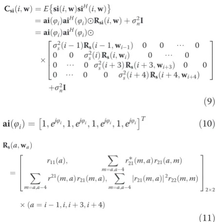
The corresponding weight covariance matrix can be given by
Csiði;wÞ ¼Esiði;wÞsiHði;wÞ ¼aið Þφi aiH φ
i
ð Þ⊙Rsiði;wÞ þσ2nI
¼aið Þφi aiHð Þφi ⊙
σ2
sði1ÞRsði1;wi1Þ 0 0 ⋯ 0 0 0 σ2
sð Þi Rsði;wiÞ 0 ⋯ 0 0 ⋯ 0 σ2
sðiþ3ÞRsðiþ3;wiþ3Þ 0 0
0 ⋯ 0 0 σ2
sðiþ4ÞRsðiþ4;wiþ4Þ
2 6 6 4
3 7 7 5
þσ2
nI
ð9Þ
aið Þ ¼φi 1;ejφi;1;ejφi;1;ejφi;1;ejφi
T
ð10Þ
Rsða;waÞ
¼
r11ð Þa;
X
m¼a;a4 r∗
21ðm;aÞr21ða;mÞ X
m¼a;a4
r21ðm;aÞr 21ðm;aÞ;
X
m¼a;a4 r21ðm;aÞ
j j2r 22ðm;mÞ 2
6 6 4
3 7 7 5
22
ða¼i1;i;iþ3;iþ4Þ
ð11Þ
where Rsi(i,w) is called the weight correlation function
matrix of the pixel pairi.
In the following, the characteristics of the signal and the noise subspaces of the weight covariance matrix Csi(i,w)
for different coregistration errors are discussed.
When the example of formula (1) is used to build the data vector, the correlation coefficient of the corresponding
item of the data vector decreases with the increasing coregistration error. On the contrary, the correlation coef-ficient is not impacted by the coregistration error when the correlation weight data vector is used. That means the cor-relation coefficient [i.e., the cross-corcor-relation coefficients of
Rs(a,wa) (a=i –1, i,i + 3, i+ 4)] of the corresponding item of the correlation weight data vector with the coregistration errorμ(0 < μ≤1) pixel is as high as that of the corresponding item of the data vector with accurate coregistration. Figure 2 shows the correlation coefficient for various data vector versus the coregistration error to further demonstrate the above conclusions.
From the literature [14,19], we know that the rank ofRs
(a,wa)(a=i–1,i,i+ 3,i+ 4) becomes 1 when the cross-correlation coefficients (i.e., the non-diagonal elements) of
Rs(a,wa)(a=i–1,i,i+ 3,i+ 4) are high enough. There-fore, the number of the principal eigenvalues ofRsi(i,w) is
4 according to (9), and the number of the principal eigenvalues of Csi(i,w) is also equal to 4 [14]. That is the
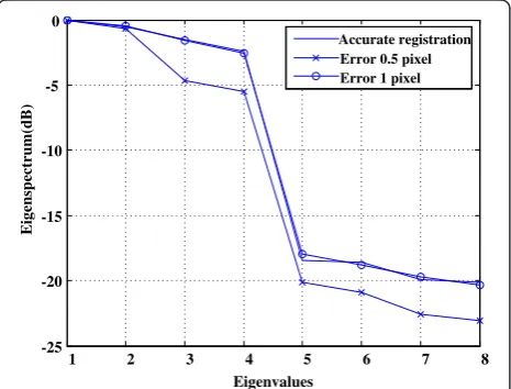
dimensions of the signal subspace and the noise subspace are both 4 in the presence of large coregistration errors. Figure 3 shows the eigenspectra of the weight covariance matrix for different coregistration errors to further dem-onstrate the above conclusions.
In this case, the eigendecomposition of the weight co-variance matrixCsi(i,w) is as follows:
Csiði;wÞ ¼Esiði;wÞsiHði;wÞ
¼aið ÞφiaiHð Þφi ⊙Rsiði;wÞ þσ2nI
――
――
EVDX4 k¼1
λð Þcsik βð Þcsik βð ÞcsikHþX4 l¼1
σ2 nβð Þnsilβð ÞnsilH
¼X4 k¼1
λð Þrsik þσ2 n
aið Þφi⊙βð Þrsik
aið Þφi ⊙βð Þrsik
H
þX
4
l¼1 σ2
nβð Þnsil βð ÞnsilH
ð12Þ 1
SAR SAR2
i 1 i
5
i i 4
3
i i 4
1
i
i
3
i i 4
1 2 1 2 1 2 1 2
1 1 1 1 1 3 3 1 4 4
( , )
[ (
1),
(
1), ( ),
( ), (
3),
(
3), (
4),
(
4)]
[ (
1),
, ( ),
, (
3),
, (
4),
]
T W
W W
W
T T T
T T
i i i i i i i i
i
s i
s
i
s i s
i s i
s
i
s i
s
i
s i
s i
s i
s i
si
w
w V
w V
w V
w
V
where βcsi(k)(k = 1, 2, 3, 4) is the eigenvector corres-ponding to the principal eigenvalue λcsi(k)(k = 1, 2, 3, 4) of Csi(i,w), βrsi(k)(k = 1, 2, 3, 4) is the eigenvector corresponding to the principal eigenvalue λrsi(k)(k = 1, 2, 3, 4) of Rsi(i,w), σ2n and βnsi(l)(k = 1, 2, 3, 4) are the noise eigenvalue and the corresponding eigenvector of
Csi(i,w). From (12) we can note that ai(φi) ⊙ βrsi(k)(k = 1, 2, 3, 4) is in the signal subspace of Csi(i,w), βnsi(l) (k = 1, 2, 3, 4) is in the noise subspace of Csi(i,w),
and the signal subspace are orthogonal to the noise subspace [14].
From the results derived above, we can see that the new formulation of the correlation weight joint data vector proposed in this article has the advantage that the noise subspace dimension of the corresponding
weight covariance matrix is independent of the coregistration error. That is to say, the noise subspace dimension of the corresponding covariance matrix with the coregistration errorμ(0 <μ≤1) pixel is the same as that of the accurate covariance matrix (in this article, the noise subspace dimension of the corresponding co-variance matrix with the accurate coregistration is 4). Therefore, it is not required to calculate the noise sub-space dimension before estimating the InSAR interfero-metric phase, thus the introduced trouble will be avoided.
3. Processing procedures
In this section, we give the detailed steps for this proposed method.
Step 1.Coregister SAR images.
The SAR images are coarsely coregistered using the cross-correlation information of the SAR image intensity or other strategies [1,2] after SAR imaging of the echoes acquired by each satellite.
Remark 1: The required image coregistration accuracy for the proposed method can be 1 pixel, which is much lower than the required accuracy (from 1/10 to 1/100 pixel) for conventional methods. The low coregistration accuracy requirement can greatly facilitate coregistration processing.
Step 2.Estimate the covariance matrix.
An example to construct the formulation of the correl-ation weight joint data vectorjs(i,w) is shown in Figure 4 when the coregistration error isμ(0 ≤μ ≤1) pixels and its direction is unknown.
jsði;wÞ ¼ ½s1ði1Þ;s2Wði1Þ;s1ð Þi ;s2Wð Þi ;s1ðiþ3Þ; s2Wðiþ3Þ;s1ðiþ4Þ;s2Wðiþ4ÞT
¼ ½s1ði1Þ;wTi1Vi1;s1ð Þi ;wTiVi;s1ðiþ3Þ;
wT
iþ3Viþ3;s1ðiþ4Þ;wTiþ4Viþ4T where
Va¼ ½s2ða5Þ;s2ða4Þ;s2ða3Þ;s2ða1Þ;s2ð Þa; s2ðaþ1Þ;s2ðaþ3Þ;s2ðaþ4Þ;s2ðaþ5ÞT
a¼i1;i;iþ3;iþ4
ð Þ
ð13Þ
wa¼ ½^r21ða5;aÞ;^r21ða4;aÞ;^r21ða3;aÞ;
^
r21ða1;aÞ;^r21ða;aÞ;^r21ðaþ1;aÞ;
^r21ðaþ3;aÞ;^r21ðaþ4;aÞ;^r21ðaþ5;aÞT a¼i1;i;iþ3;iþ4
ð14Þ
1 2 3 4 5 6 7 8
-25 -20 -15 -10 -5 0
Eigenvalues
Eigensp
ect
ru
m
(dB
)
Accurate registration Error 0.5 pixel Error 1 pixel
Figure 3Eigenspectra of the weight covariance matrix for accurate coregistration, coregistration errors of 0.5 and 1 pixels, respectively.
0.2 0.4 0.6 0.8 1
0 0.1 0.2 0.3 0.4 0.5 0.6 0.7 0.8 0.9
Coregistration error(pixel)
correlation coefficient
correlation weight data vector data vector build using formula (1)
^r21ðm;aÞ ¼
XK
k¼K
s2ðmþkÞs1ðaþkÞ
ffiffiffiffiffiffiffiffiffiffiffiffiffiffiffiffiffiffiffiffiffiffiffiffiffiffiffiffiffiffiffiffiffiffiffiffiffiffiffiffiffiffiffiffiffiffiffiffiffiffiffiffiffiffiffiffiffiffiffiffiffiffiffiffiffiffiffi
XK k¼K
s2ðmþkÞ
j j2XK
k¼K
s1ðiþkÞ
j j2
v u u t
m¼a5;a4;a3;a1;a;aþ1;aþ3;aþ4;aþ5
a¼i1;i;iþ3;iþ4
ð15Þ
The corresponding weight covariance matrix can be given by
Cjsði;wÞ ¼Efjsði;wÞjsHði;wÞg
¼aið Þaiφi Hð Þφ;i ⊙Rjsði;wÞ þσ2nI ð16Þ
where Rjs(i,w) is called the weight correlation function matrix of the pixel pairi. Under the assumption that the neighboring pixels have the identical terrain height and the complex reflectivity is independent from pixel-to -pixel [16], the weight covariance matrix Cjs(i,w) given by (16) can be estimated by its sample covariance matrix
C^jsði;wÞ, i.e.,
C^jsði;wÞ ¼ 1 2Kþ1
XK
k¼K
jsðiþk;wÞjsHðiþk;wÞ
ð17Þ
where 2 K+ 1 is the number of i.i.d. samples from the neighboring pixel pairs.
Remark 2: According to the Reed–Mallett–Brennan rule [20], the effective number of looks (i.e., the num-ber of i.i.d. samples) that 2 K + 1 ≥ 2 M – 1 would
make the estimation loss within 3 dB if the
dimensions of the covariance matrix C^jsði;wÞareM×M. The detailed analysis of the effective number of looks is presented in [21].
It is easy to obtain enough i.i.d. samples for locally flat terrains. However, an imaging terrain in practice cannot be relied upon to be so flat that the adjacent pixels have the identical terrain height. If the local terrain slope is available in advance or can be estimated [15], the steering vector (i.e., the interferometric phase) variation due to the different terrain height from pixel-to-pixel can be compensated, which greatly enlarges the size of the sample window.
Step 3.Subspace estimation by eigendecomposing. The estimated covariance matrix C^jsði;wÞof the dimen-sions 8 × 8 can be eigendecomposed into
C^jsði;wÞ ¼ XK
k¼1
^ λð Þcjskβ
^ð Þk
cjsβ
^ð ÞkH
cjsi þ X
8K
l¼1
^
λðcjslþKÞβ
^ð Þl
njsβ
^ð ÞlH
njs
ð18Þ
where K (in this article, K is equal to 4) is the number of the principal eigenvalues of C^jsði;wÞ, ^
λð Þcjs1 >^λ 2
ð Þ
cjs >⋯>^λ K
ð Þ
cjs >>^λ Kþ1
ð Þ
cjs >⋯>^λ 8
ð Þ
cjs ,
eigen-vectors β
^ð Þl
njsðl¼1;2;. . .;8KÞ corresponding to the smaller eigenvalues λ^ðcjslþKÞðl¼1;2;. . .;8KÞ span the noise subspace, i.e.,
Nc¼span β ^ð Þ1
njs;β
^ð Þ2 njs;. . .;β
^ð8KÞ
njs
ð19Þ
whereas the larger eigenvectors β
^ð Þk
cjsðk¼1;2;. . .;KÞ corresponding to the principal eigenvalues ^λð Þcjskðk¼1;2; . . .;KÞspan the signal subspace, i.e.,
Sc¼span β ^ð Þ1
cjs;β
^ð Þ2 cjs;. . .;β
^ð ÞK
cjs
ð20Þ
1 2 1 2 1 2 1 2
1 1 1 1 1 3 3 1 4 4
( , )
[ (
1),
(
1), ( ),
( ), (
3),
(
3), (
4),
(
4)]
[ (
1),
, ( ),
, (
3),
, (
4),
]
T W
W
W W
T T T
T T
i i i i i i i i
i
s i
s
i
s i s
i s i
s
i
s i
s
i
s i
s i
s i
s i
js
w
w V
w V
w V
w V
2 SAR
i 1
i
i i 1
i 6i 5i 4i 3
i 2 i 3i 4i 5
i 6 i 7i 8i 9 2
1 SAR
1
i
i
i 3i 4
The noise power is often estimated by [14]
^
σn2¼81K X
8K l¼1
^
λðcjslþKÞ ð21Þ
The joint correlation function matrix R^jsði;wÞ can be approximated as the amplitude (i.e., the absolute value) of the estimated covariance matrix C^jsði;wÞ[14], i.e.,
R^jsði;wÞ ¼C^jsði;wÞ ^σ2nI ð22Þ
By eigendecomposing R^jsði;wÞ, we obtain K principal
eigenvectors β^k
ð Þ
rjsðk¼1;2;. . .;KÞ. As shown by (12), the
same signal subspace spanned by the principal eigenvectors
β^ð Þk
cjsðk¼1;2;. . .;KÞ of C^jsði;wÞ can be spanned by the
Hadamard product vectorsaið Þφi ⊙β ^ð Þk
rjsðk¼1;2;. . .;KÞ, i.e.,
Sc¼span aið Þφi ⊙β
^ð Þ1
rjs;aið Þφi ⊙β ^ð Þ2
rjs;. . .;aið Þφi ⊙β ^ð Þk
rjs
ð23Þ
Step 4. Projection of signal subspace onto noise subspace.
As mentioned above, the signal subspace is orthogonal to the noise subspace, which is used to estimate the interferometric phaseϕi.
Definition of cost function:
J¼XK
k¼1
X
8K l¼1
aið Þφi ⊙β
^ð Þk
rjsÞ H
β^ð Þl
njsβ
^ð ÞlH
njs aið Þφi ⊙β ^ð Þk
rjs
ð24Þ
where
aið Þ ¼φi 1;ejφi;1;ejφi;1;ejφi;1;ejφi
T
ð25Þ
The minimization of J can provide the optimum esti-mate of the interferometric phaseϕi, i.e.,φ^i¼φi.
Remark 3: The computational burden will be high if the minimization ofJ is obtained via search of ϕiin the principal phase interval [−π, +π]. To reduce the compu-tational burden, a fast algorithm to compute the minimization of J is developed in Appendix, where the closed-form solution to the estimate of φi is directly obtained by using the fast algorithm.
With the use of the above four steps, the terrain inter-ferogram can be recovered after the pixel pairs of the SAR images are processed separately.
4. Performance investigation
In this section, we demonstrate the robustness of the method to coregistration errors by using two sets of simulated data and a real dataset.
We assume that there are two formation-flying satellites in the cartwheel formation, and we select one orbit pos-ition for simulation, with an effective cross-track baseline of 562.93 m, an orbit height of 750 km, and an incidence angle of 50°. We use a two-dimensional Hann window to simulate the terrain and use the statistical model to gener-ate the complex SAR image pairs [22]. The signal-to-noise ratio of the SAR images is 16 dB.
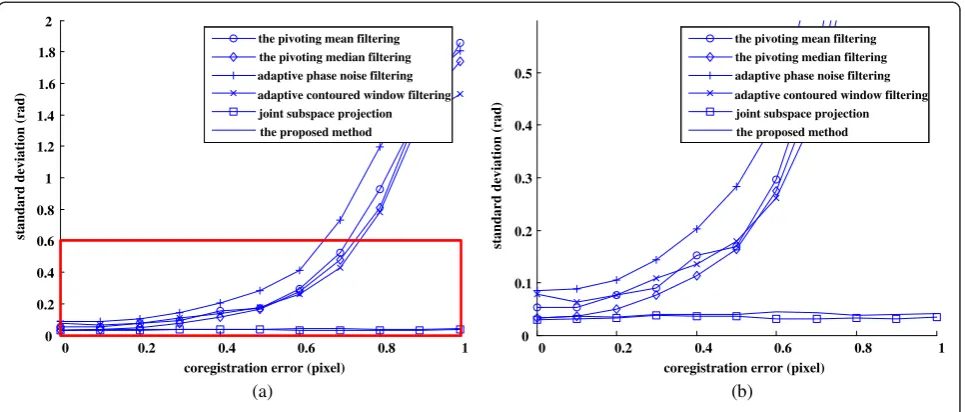
Here, the number of the samples to estimate the co-variance matrix is 7 (in range) × 7 (in azimuth) = 49. The variation of the standard deviation of the interfero-metric phase with the increasing coregistration error was computed by means of 1,000 Monte Carlo simulations.
Figures 5, 6, and 7 compare the simulation results for various techniques and coregistration errors. Compar-ing Figures 5, 6, and 7, we can observe that the large coregistration error heavily affects the interferograms obtained by pivoting mean filtering, pivoting median filtering, adaptive phase noise filtering, and adaptive contoured window filtering. On the contrary, the large coregistration error has almost no effect on the inter-ferograms obtained by the proposed method. We can see that the proposed method in this article is robust to large coregistration errors (up to 1 pixel).
Now we demonstrate the robustness of the method to local misregistration [16] (note that by “local mis-registration” we mean that the coregistration error is not same for every image pixel) using the simulated data above.
Figure 8 shows the interferograms obtained by various techniques for the local misregistration. From the simula-tion results, we can observe that the local misregistrasimula-tion heavily affects the interferograms obtained by pivoting mean filtering, pivoting median filtering, adaptive phase noise filtering, and adaptive contoured window filtering. However, the proposed method is robust to the increasing coregistration error. In other words, our method can ac-curately estimate the corresponding terrain interferomet-ric phase in the presence of the local misregistration.
Figure 9 shows the variation of the standard deviation of the interferometric phase with the increasing co-registration error. We can see that the performance of our method is as good as that of the joint subspace pro-jection method [14]. However, our method can avoid the trouble of calculating the noise subspace dimension before estimating the InSAR interferometric phase.
50 100 150 200 250 300 350 400 450 500 100
200
300
400
500
600
50 100 150 200 250 300 350 400 450 500 100
200
300
400
500
600
50 100 150 200 250 300 350 400 450 500 100
200
300
400
500
600
R
ange
(pixe
l)
Azimuth (pixel)
Rang
e(p
ixe
l)
Azimuth(pixel)
Range(pixel)
Azimuth(pixel)
(a)
(b)
(c)
50 100 150 200 250 300 350 400 450 500 100
200
300
400
500
600
50 100 150 200 250 300 350 400 450 500 100
200
300
400
500
600
R
a
nge(p
ixe
l)
Azimuth(pixel)
Range(pixel)
Azimuth(pixel)
(d)
(e)
Figure 6Image coregistration error of 0.5 pixels.Interferograms obtained by (a) pivoting mean filtering, (b) pivoting median filtering, (c) adaptive phase noise filtering, (d) adaptive contoured window filtering, and (e) the proposed method.
Range(pixel)
Azimuth(pixel)
50 100 150 200 250 300 350 400 450 500
100
200
300
400
500
600
Azimuth(pixel)
50 100 150 200 250 300 350 400 450 500
Range
(p
ixe
l)
Azimuth(pixel)
50 100 150 200 250 300 350 400 450 500
100
200
300
400
500
600
R
a
n
ge(pixel)
100
200
300
400
500
600
Range(pixel)
Azimuth(pixel)
50 100 150 200 250 300 350 400 450 500
100
200
300
400
500
600
R
ange
(pi
x
el)
Azimuth(pixel)
50 100 150 200 250 300 350 400 450 500
100
200
300
400
500
600
(e)
(d)
(b)
(a)
(c)
50 100 150 200 250 300 350 400 450 500 100
200
300
400
500
600
50 100 150 200 250 300 350 400 450 500 100
200
300
400
500
600
50 100 150 200 250 300 350 400 450 500 100
200
300
400
500
600
Range
(pixel)
Azimuth (pixel)
R
ang
e(
pixel)
Azimuth (pixel)
Rang
e(
pixe
l)
Azimuth (pixel)
(a)
(b)
(c)
50 100 150 200 250 300 350 400 450 500 100
200
300
400
500
600 50 100 150 200 250 300 350 400 450 500 100
200
300
400
500
600
R
a
n
ge
(pi
x
el
)
Azimuth (pixel)
Ra
ng
e(pixel
)
Azimuth(pixel)
(d)
(e)
Figure 8Local misregistration.Interferograms obtained by (a) pivoting mean filtering, (b) pivoting median filtering, (c) adaptive phase noise filtering, (d) adaptive contoured window filtering, and (e) the proposed method.
50 100 150 200 250 300 350 400 450 500 100
200
300
400
500
600
50 100 150 200 250 300 350 400 450 500 100
200
300
400
500
600
50 100 150 200 250 300 350 400 450 500 100
200
300
400
500
600
R
a
nge
(pix
el)
Azimuth (pixel)
Range(pixe
l)
Azimuth (pixel)
R
a
nge(pixel)
Azimuth (pixel)
(a)
(b)
(c)
50 100 150 200 250 300 350 400 450 500 100
200
300
400
500
600 50 100 150 200 250 300 350 400 450 500 100
200
300
400
500
600
Ra
n
ge
(pixel)
Azimuth (pixel)
Range(p
ixel)
Azimuth (pixel)
(d)
(e)
Figure 10 shows the interferograms generated from the Mount Etna data. Figure 10a is the interferogram obtained by conventional processing [16] (i.e., directly computing the interferometric phase pixel-by-pixel), and Figure 10b is the interferogram obtained by the ap-proach proposed in this article.
Figure 11 confirms the effectiveness of the proposed method in processing of the ERS1/ERS2 (European Re-mote Sensing 1 and 2 tandem satellites, ERS1 orbit = 32585, ERS2 orbit = 12912, frame = 2781, 1997-10-08/ 09, Zhangbei, China) real data.
Figure 11 shows the interferograms generated from the ERS1/ERS2 real data. Figure 11a is the interferogram obtained by conventional processing, and Figure 11b is
the interferogram obtained by the approach proposed in this article.
5. Conclusions
We have proposed a new method to estimate the terrain interferometric phases from the InSAR image pair. Bene-fiting from the new formulation of correlation weight joint data vector, the method does not need to calculate the noise subspace dimension before estimating the InSAR interferometric phase, thus the introduced trouble will be avoided. The method is based on the projection of the joint signal subspace onto the corresponding joint noise subspace, and takes advantage of the coherence informa-tion of the neighboring pixel pairs to auto-coregister the
0 0.2 0.4 0.6 0.8 1
0 0.2 0.4 0.6 0.8 1 1.2 1.4 1.6 1.8 2
coregistration error (pixel)
st
a
nd
ard
d
evi
ati
o
n
(ra
d
)
the pivoting mean filtering the pivoting median filtering adaptive phase noise filtering adaptive contoured window filtering joint subspace projection the proposed method
0 0.2 0.4 0.6 0.8 1
0 0.1 0.2 0.3 0.4 0.5
coregistration error (pixel)
standard
deviation
(rad)
the pivoting mean filtering the pivoting median filtering adaptive phase noise filtering adaptive contoured window filtering joint subspace projection the proposed method
(a) (b)
Figure 9Standard deviation of the interferometric phase versus the coregistration error.
Range(pixel)
Azimuth(pixel)
100 200 300 400 500 600 700 100
200
300
400
500
600
700
R
ange
(p
ixe
l)
Azimuth(pixel)
100 200 300 400 500 600 700 100
200
300
400
500
600
700
(a)
(b)
SAR images, where the phase noise is reduced simultan-eously. A fast algorithm is developed to implement the method, which can significantly reduce the computational burden. The effectiveness of the method is verified via simulated data and real data.
Appendix
Fast algorithm to compute the optimum interferometric phase estimate
If U,V, and W are arbitrary complex column vectors, then [14]
U⊙V
ð ÞHW⋅WHðU⊙VÞ
¼UHhW⋅WH⊙V∗⋅ðV∗ÞHiU ð
26Þ
Using Equation (26), we can rewrite the cost function of (24) as
J¼XK
k¼1
X
8K
l¼1
aið Þφi⊙β^k ð Þ rjs
H
^
βð Þnjsl^βnjsð ÞHl aið Þφi⊙^βk ð Þ rjs
¼XK
k¼1
X
8K
l¼1 aiH φ
i
ð Þ β^ð Þnjsl^βl ð Þ njsH
⊙ ^βð Þrjsk∗ ^βk ð Þ rjs∗
H
aið Þφi
¼aiH φ i
ð Þ XK
k¼1
X
8K
l¼1 ^
βð Þnjsl^βð ÞnjslH
⊙ ^βð Þrjsk∗ ^βð Þrjsk∗
H
( )
aið Þφi
ð27Þ
Let A¼X
K
k¼1
X
8K l¼1
^ βð Þnjsl ^βl
ð Þ
njsH
⊙ ^βð Þrjsk∗ ^βk
ð Þ
rjs∗
H
. It
can easily be proved thatA(8 × 8) is a Hermitian matrix.
Then (27) can be rewritten as
J¼aiH φ i ð Þ XK
k¼1
X
8K
l¼1 ^
βð Þnjsl^βð ÞnjslH
⊙ ^βð Þrjsk∗ β^ð Þrjsk∗
H
( )
aið Þφi
¼aiH φ i ð ÞAaið Þφi
¼ βH φ i ð Þ;βH φ
i ð Þ;βH φ
i ð Þ;βH φ
i ð Þ
A1 A2 A3 A4 A5 A6 A7 A8 A9 A10 A11 A12 A13 A14 A15 A16
2 6 6 4 3 7 7 5
βð Þφi βð Þφi
βð Þφi βð Þφi
2 6 6 4 3 7 7 5
¼X16 m¼1
βH φ i
ð ÞAmβð Þφi
¼βH φ i ð Þ X4
m¼1 Am
( )
βð Þφi
ð28Þ
where
βð Þ ¼φi 1;ejφi
T
ð29Þ
LetB¼X
16
m¼1
Am¼ bb11 b12 21 b22
. It can easily be proved
that Bis a Hermitian matrix, i.e., b12∗ = b21, Let b12 = | b12|ejμ. Then,
J ¼βH φ i
ð Þ X
16
m¼1
Am
( )
βð Þ ¼φi βHð ÞBφi βð Þφi
¼½1;ejφi b11 b12 b21 b22
1 ejφi
¼b11þb22þb21ejφiþb12ejφi
¼b11þb22þðjb12jejμ⋅ejφiÞ∗þjb12jejμ⋅ejφi
¼b11þb22þ2jb12jcosðμþφiÞ
ð30Þ Range(pixel)
Azimuth(
p
ixel)
500 1000 1500 2000
200 400 600 800 1000 1200 1400 1600 1800 2000 2200 Range(pixel) Azimuth(p ixe l)
500 1000 1500 2000
200 400 600 800 1000 1200 1400 1600 1800 2000 2200
(a)
(b)
Obviously, the minimization of J can be obtained for μ +φi =−π + 2kπ(k is an integer and μ= angle(b12)). Since–π≤μ<πand–π<φi<π, thus
φi¼ ππμμ ððμμ≤>0Þ0Þ
ð31Þ
Endnotes a
As shown in Figure 1, the horizon is along range and the verticality is along azimuth.
b
Epsilon Nought, Radar Remote Sensing: http://epsilon. nought.de/.
Competing interests
The authors declare that they have no competing interests.
Acknowledgements
This paper was supported by the National Natural Science Foundations of China under grant 61071194, 60979002 and 61231017, by the Fund of Civil Aviation University of China under grant 2011kyE06, and the National Key Technology Research and Development Program of China (2011BAH24B12).
Received: 27 June 2012 Accepted: 5 February 2013 Published: 20 February 2013
References
1. PA Rosen, S Hensley, IR Joughin, FK Li, SN Madsen, E Rodrìguez, RM Goldstein, Synthetic aperture radar interferometry. Proc. IEEE88(3), 333–382 (2000)
2. R Bamler, P Hartl, Synthetic aperture radar interferometry. Inverse Probl.
14, R1–R54 (1998)
3. Q Lin, JF Vesecky, HA Zebker, Registration of Interferometric SAR Images, in Proceedings of the International Geoscience and Remote Sensing
Symposium’1992, Houston, Texas, USA, vol. 2, 1992, pp. 1579–1581 4. R Scheiber, A Moreira, Coregistration of interferometric SAR images using
spectral diversity. IEEE Trans. Geosci. Remote Sens.38(5), 2179–2191 (2000) 5. D Fernandes, G Waller, JR Moreira, Registration of SAR images using the
chirp scaling algorithm, inProceedings of th International Geoscience and Remote Sensing Symposium’1996, Lincoln, NE, USA, vol. 1, 1996, pp. 799–801 6. X Wei, C Ian, A region-growing algorithm for InSAR phase unwrapping. IEEE
Trans. Geosci. Remote Sens.37(1), 124–134 (1999)
7. M Costantini, A novel phase unwrapping method based on network programming. IEEE Trans. Geosci. Remote Sens.36(3), 813–831 (1998) 8. RM Goldstein, HA Zebker, CL Werner, Satellite radar interferometry:
two-dimensional phase unwrapping. Radio Sci.23(4), 713–720 (1988) 9. MD Pritt, JS Shipman, Least-squares two-dimensional phase unwrapping
using FFT’s. IEEE Trans. Geosci. Remote Sens.32(3), 706–708 (1994) 10. PH Eichel, DC Ghiglia, CV Jakowatz Jr, PA Thompson, DE Wahl, Spotlight
SAR interferometry for terrain elevation mapping and interferometric change detection. Sandia National Labs Technical Report, SAND93, 2539–2546 (1993)
11. R Lanari, G Fornaro, D Riccio, M Migliaccio, KP Papathanassiou, JR Moreira, M Schwabisch, L Dutra, G Puglisi, G Franceschetti, M Coltelli, Generation of digital elevation models by using SIR-C/X-SAR multifrequency two-pass interferometry: the Etna case study. IEEE Trans. Geosci. Remote Sens.34(5), 1097–1114 (1996)
12. J-S Lee, KP Papathanassiou, TL Ainsworth, MR Grunes, A Reigber, A new technique for noise filtering of SAR interferometric phase images. IEEE Trans. Geosci. Remote Sens.36(5), 1456–1465 (1998)
13. Y Qifeng, X Yang, F Sihua, X Liu, X Sun, An adaptive contoured window filter for interferometric synthetic aperture radar. IEEE Geosci. Remote Sens. Lett.4(1), 23–26 (2007)
14. L Zhenfang, B Zheng, L Hai, L Guisheng, Image auto-coregistration and InSAR interferogram estimation using joint subspace projection. IEEE Trans. Geosci. Remote Sens.44(2), 288–297 (2006)
15. H Li, Z Li, G Liao, Z Bao, An estimation method for InSAR interferometric phase combined with image auto-coregistration. Sci. China, Ser. F.49(3), 386–396 (2006)
16. H Li, G Liao, An estimation method for InSAR interferometric phase based on MMSE criterion. IEEE Trans. Geosci. Remote Sens.48(3), 1457–1469 (2010) 17. F Lombardini, M Montanari, F Gini, Reflectivity estimation for multibaseline
interferometric radar imaging of layover extended sources. IEEE Trans. Signal Process.51(6), 1508–1519 (2003)
18. L Hai, L Guisheng, A phase unwrapping method for multibaseline InSAR systems based on correlation coefficient weight data vector. Prog. Nat. Sci. (in Chinese)18(3), 313–322 (2008)
19. L Hai, W Renbiao, InSAR interferometric phase estimation based on correlation weight subspace projection, in2011 IEEE CIE International Conference on Radar, Chengdu, China, vol. 1, 2011, pp. 398–401
20. IS Reed, JD Mallett, LE Brennan, Rapid convergence rate in adaptive arrays. IEEE Trans. Aerosp. Electron. Syst.10, 853–863 (1974)
21. CH Gierull, IC Sikaneta, Estimating the effective number of looks in interferometric SAR data. IEEE Trans. Geosci. Remote Sens.40(8), 1733–1742 (2002)
22. F Lombardini, Absolute phase retrieval in a three-element synthetic aperture radar interferometer, inProceedings of the 1996 CIE International Conference on Radar, Beijing, China, 1996, pp. 309–312
doi:10.1186/1687-6180-2013-27
Cite this article as:Li and Wu:An estimation method for InSAR
interferometric phase using correlation weight joint subspace projection.EURASIP Journal on Advances in Signal Processing20132013:27.
Submit your manuscript to a
journal and benefi t from:
7 Convenient online submission 7 Rigorous peer review
7 Immediate publication on acceptance 7 Open access: articles freely available online 7 High visibility within the fi eld
7 Retaining the copyright to your article