S
TRATHCLYDE
DISCUSSION PAPERS IN ECONOMICS
DEPARTMENT OF ECONOMICS
UNIVERSITY OF STRATHCLYDE
GLASGOW
INVERTED HAAVELMO EFFECTS IN A GENERAL
EQUILIBRIUM ANALYSIS OF THE IMPACT OF
IMPLEMENTING THE SCOTTISH VARIABLE RATE OF
INCOME TAX.
BY
PATRIZIO LECCA, PETER G MCGREGOR, KIM SWALES
AND YA PING YIN.
Inverted Haavelmo Effects in a General Equilibrium Analysis of
the Impact of Implementing the Scottish Variable Rate of Income
Tax.
*by
Patrizio Leccab Peter G. McGregora
J. Kim Swalesb Ya Ping Yinc
a
Fraser of Allander Institute, Department of Economics, University of Strathclyde b
Department of Economics, University of Strathclyde c
Department of Statistics, Economics, Accounting and Management Systems, University of Hertfordshire
*
The authors gratefully acknowledge the support of the ESRC (grant L219252102) under the Devolution and
Constitutional Change Research Programme. We thank Brian Ashcroft, Steve Bailey, Ayele Gelana, Gary
Gillespie, Jim Stevens and Karen Turner for help in the preparation of this paper and for comments on previous
drafts. We are also grateful to participants in seminars given on related material at Lancaster, Stirling and
Abstract
The Scottish Parliament has the authority to make a balanced-budget expansion or contraction in public expenditure, funded by corresponding local changes in the basic rate of income tax of up to 3p in the pound. This fiscal adjustment is known as the Scottish Variable Rate of income tax, though it has never, as yet, been used. In this paper we attempt to identify the impact on aggregate economic activity in Scotland of implementing these devolved fiscal powers. This is achieved through theoretical analysis and simulation using a Computable General Equilibrium (CGE) model for Scotland. This analysis generalises the conventional Keynesian model so that negative balanced-budget multipliers values are possible, reflecting a regional “inverted Haavelmo effect”. Key parameters determining the aggregate economic impact are the extent to which the Scottish Government create local amenities valuable to the Scottish population and the extent to which this is incorporated into local wage bargaining.
JEL Numbers: C68, D58, H71, R13, R23
1. INTRODUCTION
In 1997 the Scottish people voted to create a Scottish legislative assembly and to endow that body with tax-varying powers. Subsequently the Scotland Act (1998) established the Scottish Parliament and gave it the authority to make a balanced-budget expansion or contraction in public expenditure. This local fiscal adjustment would be funded by corresponding local changes in the basic rate of income tax of up to 3p in the pound. This is known as the Scottish Variable Rate of income tax, though it has never, as yet, been used. In this paper we attempt to identify and quantify the impact on aggregate economic activity in Scotland of implementing these devolved fiscal powers. This is achieved through theoretical analysis and simulation using a Computable General Equilibrium (CGE) model for Scotland.
The bulk of the funding for the Scottish Parliament comes through a block grant from the UK Government determined by the Barnett formula (Bell et al, 1997; Christie and Swales, 2010). According to official data, Scotland has higher per capita public expenditure than England and is generally thought to receive a substantial positive net fiscal transfer from the rest of the UK.1 This leads most commentators to believe that for Scotland the power to change the standard rate of income tax is, in practice, restricted to the power to increase it (Blow et al, 1996; McGregor et al 1997). We therefore focus here specifically on the consequences for the Scottish economy of a balanced-budget fiscal expansion.
Since Scottish devolution there has been an active, and often animated, debate about the funding of those expenditures controlled by the Scottish Parliament (Ashcroft et al, 2006; Bell, 2000; Christie and Swales, 2010; Cuthbert, 1998, 2001; Gallacher and Hinze, 2005; Hallwood and MacDonald, 2005, 2006; McLean and McMillan, 2003; Midwinter 1999, 2002)).2
1 The size of Scotland’s fiscal balance is not uncontested and depends on the treatment of the taxation associated with the extraction of North Sea oil (Scottish Government, 2010).
The Commission on Scottish Devolution (2009), chaired by Kenneth Calman, inter alia recommends that the extent to which the Scottish Government can vary the rates on a number of existing taxes should be significantly extended. The most important is income tax and the the report proposed a variation of up to 10p in the pound. But the key recommendation was
that the Scottish Parliament be forced to choose the appropriate income tax rate rather than have the present default position of accepting the rate set at the UK level. In the budget of 2010, the Coalition Government affirmed its commitment to implement the proposals of the Calman Commission in Scotland. A similar position had been taken in the Labour Government’s budget earlier in the same year.3
In this paper we concentrate on the impact of the operation of the Scottish Variable Rate. However, the recommendations of the Calman Commission relating to the expanded powers for devolved income tax setting are essentially as analysed here, except that the size of the allowable tax change will be increased. An obvious reference point for our analysis is the fiscal federalism literature (Cornes and Sandler, 1996, ch. 11; Oates, 1972, 1999;). However, the micro-theoretic literature assumes that greater fiscal autonomy will have a neutral impact on regional macro-economies. We argue that there can be no such presumption in the UK regional context. Further, it is not possible, a priori, to determine the sign of the change in regional activity that would be generated by a balanced budget fiscal expansion at the regional level.
Section 2 outlines our theoretical approach. We adopt an explicitly general equilibrium variant of the disaggregated Layard et al. (1991) model, augmented to allow for the effect on regional wage determination and migration of regional-specific tax-funded amenities. Section 3 uses this analysis to generalise the conventional Keynesian balanced-budget multiplier model. In this setting, negative balanced-budget multipliers values are possible, reflecting a regional “inverted Haavelmo effect” (Haavelmo, 1945; Knoester and van der Windt, 1987). Section 4 identifies the structure of AMOS, a Computable General Equilibrium (CGE) model parameterized on data for Scotland. This is a fleshed out version of the skeletal theoretical model set out in Section 3,. Section 5 reports the simulation results for the impact of the introduction of the Scottish Variable Rate on long-run equilibria, and Section 6 explores a number of extensions. Section 7 concludes with the implications for future research and for the
3 The Independent Commission on Funding and Finance for Wales (2010), chaired by Gerry Holtham has
similarly argued, inter alia, for the Welsh Assembly to have the power to change the basic rate of income tax
wider debate on regional fiscal issues.
2. THE THEORETICAL MODEL
We adopt a long-run, open-economy model of the region which is in the spirit of the disaggregated approach developed by Layard et al. (1991, ch. 6) with imperfect competition in the regional labour market. We employ the small-region assumption that the price of imports and the cost of capital are both determined exogenously in perfectly integrated national/international markets. However, we do not impose the law of one price for the region's exports but rather employ conventional trade functions (Armington, 1969; Engle and Rogers, 1996). That is to say, whilst output is produced under conditions of perfect competition within the region, it is not a perfect substitute for the output of other regions.4 This permits adjustments in the price of the regional good relative to the price of extra-regional goods and allows variation in the extra-regional real and nominal wage in the long run.
Production occurs under a well-behaved, linear homogeneous production function with two factors, capital and labour. Households are assumed to be homogeneous, so that there is no distinction between workers and citizens or migrants and non-migrants. In this section and the next we focus on a comparative-static long-run analysis where equilibrium implies that both the regional capital stock and population are optimally adjusted. There is zero net investment and zero net migration in long-run equilibrium states. We adopt the Layard et al (1991) regional migration function, in which net migration is a positive function of the inter-regional relative real wage and employment rates.5 Capital stock is fully adjusted when actual and desired capital stocks in all sectors are equal.
We approach the analysis of the balanced-budget fiscal expansion (henceforth fiscal expansion) in the following way. The precise composition of the additional expenditure to be financed by the Scottish Variable Rate is unknown. However, we assume such a fiscal
4 Layard et al (1991, ch. 6) also assume competitive commodity markets in their exposition of disaggregated
labour markets.
5 This function has its roots in Harris and Todaro (1970) and has been widely employed elsewhere. See for
expansion has a positive demand-side impact on regional output through a variant of the standard balanced budget multiplier. However, there are likely to be accompanying negative supply-side effects. In particular, we assume that the increased government expenditure generates a regional-specific amenity whose existence is generally reflected in a shift in the zero net migration function (Tiebout, 1956). We argue that in an imperfectly competitive labour market the fiscal expansion also affects the real wage bargaining function. We focus on the key role played by the nature of these labour market effects in determining changes in aggregate regional activity consequent upon the introduction of the fiscal expansion. We begin with a more detailed specification of our analytical model.
Equation (1) is the zero net migration condition. It identifies the set of values of the post-tax real consumption wage, w, and the employment rate, e, for which net migration is zero:
(1 ) ( ) 0;1 0; e 1; , 0
w= −τ βz e β ≥ > ≥τ z < w wβ τ ≤ (1)
whereτ is the proportionate rate of income tax and β is a parameter indicating the degree to which households value public, as against private, consumption. Equation (1) indicates that there is a negative relationship between the post-tax real wage and the employment rate: across zero net migration (long-run) equilibria, a high local wage is compensated for by a low local employment rate. However, equation (1) is rather unconventional in that it includes the term
β
τ) 1
( − in an attempt to capture the effect on the migration decision of the locally financed amenity.
Where individuals attach no value to this amenity, β = 0 and the standard formulation of the net migration condition applies, with the post-tax real consumption wage governing migration decisions. However if, as is emphasised in the literature on fiscal federalism, there is a positive amenity effect, then β > 0, and the value of this parameter measures the potential migrant's relative marginal valuation of public expenditure versus private consumption. For a given employment rate, this implies that the larger the value of β, the lower the post-tax real consumption wage required to preclude net outmigration. When β = 1, the potential migrant is indifferent between marginal changes in local public expenditure and private consumption so that in this case the pre-tax real consumption wage drives migration.6
6 That is to say, the individual is indifferent between £1 marginal private consumption and the public good implications of paying £1 more in tax.
positive marginal preference for local public expenditure over private consumption.
The pre-tax nominal wage (W) is defined in equation (2):
τ
− ⋅ =
1 cpi w
W (2)
where cpi is the regional consumer price index defined as:
( )
0< ≤1=cpiW cpiW
cpi (3)
Equation (3) expresses the regional consumer price index as a function solely of the regional nominal wage. This parsimonious specification is permitted by the import-price and cost-of-capital exogeneity assumptions, together with the linear homogeneous nature of production.
Labour demand is given as a function of the nominal pre-tax wage and the tax rate, so that:
(
,)
0; W 0n=n W τ nτ > n < (4)
It is important to note that equation (4) represents a general equilibrium relationship, constructed on the basis of full income endogeneity. Labour demand is negatively related to the nominal pre-tax wage through competitiveness and factor substitution effects.7
On the other hand, labour demand is a positive function of the tax rate as a reflection of the operation of the conventional Keynesian balanced budget multiplier, the differential import propensities of public and private consumption expenditure, and the greater labour intensity of public sector activity.
Finally, through the bargaining function, the real consumption wage is positively related to the regional employment rate (Layard et al, 1991):
(
1)
( ) e 0, , , 0, 0 1w= −τ αβb e b > w w wα β τ ≤ ≤ ≤α (5)
In this formulation of the regional bargaining function, the local amenity generated by the expenditure is allowed to influence wage bargaining behaviour directly. The parameter α, which takes a value between 0 and 1, reflects the extent to which the value of the amenity is taken into account in the wage bargaining process.
The possible amenity effects on the local bargained real wage appear to be neglected in the literature on fiscal federalism. This is partly attributable to that literature's typical presumption of competitive labour markets. In such a situation, since the amenity provision is exogenous to the individual worker, it is ignored in the individual's work/leisure choice, so that only the post-tax real consumption wage matters.8 This corresponds to a situation where the value of α is zero. However, in the bargaining context the public good externality will be internalised in so far as local unions cover a significant section of the labour force and act co-operatively. Given that the scale of the amenity (under the proposed form of the Scottish Variable Rate) is tied directly to income and therefore to the bargained wage, the value of α will rise above zero. This formulation of the wage-setting function has echoes of the "social wage" that enjoyed some currency under earlier UK Labour administrations, although here the effect is region-specific.
3. THE THEORETICAL ANALYSIS OF THE SCOTTISH VARIABLE RATE AND OTHER FISCAL INNOVATIONS
3.1 Regional Bargained Real Wage and Flow Migration Equilibria
If equations (1)-(5) are expressed in total differentials, the change in the five endogenous variables dn, de, dcpi, dw and dW, can be determined, given the change in the value of the exogenous tax rate, dτ. The normalisation adopted is to set the initial values of w, W, and cpi
equal to unity and τ equal to zero. The relevant total differential equations are given in
Appendix 1.
A key variable in the analysis is the change in regional competitiveness that accompanies the fiscal expansion. In the present model, this is identified by the change in the nominal pre-tax wage, dW. This, together with the change in the employment rate, is determined by the interaction of the migration and bargaining functions (equations 1 and 5), suitable adopted to convert the change in real consumption wage to the change in nominal pre-tax wage. Combining equations (1), (2) and (3) produces the expression:
1
1 1
e
W W
z
dW de d
cpi cpi
β τ
−
= +
− − (6)
If dτ is set equal to zero, equation (6) gives the initial zero net migration (ZNM) function in the change in nominal pre-tax wage-employment rate space. This is represented by the curve Z0 in Figure 1, which has a slope equal to ze/(1-cpiW) < 0 and passes through the origin.
Similarly, combining equations (2), (3) and (5) expressed as total differentials gives: 1
1 1
e
W W
b
dW de d
cpi cpiαβ τ
−
= +
− − (7)
Again, setting dτ to zero in equation (7) produces the initial bargained real wage function (BRW) with a slope equal to be/(1-cpiW) > 0 which also passes through the origin. This is curve B0 in Figure 1.
Equations (6) and (7) are sufficient to tie down the change in the employment rate and
nominal wage, de and dW, that accompany the fiscal expansion, dτ:
(1 ) 0
e e
de d
b z
β −α τ
= − ≤
− (8)
and
(1 ) (1 )
(1 )( )
e e
W e e
b z
dW d
cpi b z
β αβ τ
− − −
=
− − (9)
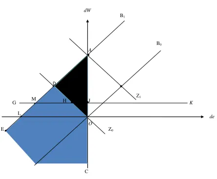
It is useful to analyse these results diagrammatically using Figure 1. Where a local income tax increase of dτ is levied, the ZNM function (equation 6) moves vertically by an amount equal to ((1-β)/(1-cpiW))dτ. The tax increase also shifts the BRW function vertically, but by ((1-αβ )/(1-cpiW))dτ. Note that the parameter restrictions imply that 1-αβ ≥1-β so that the BRW function cannot experiences a smaller upward movement than the ZNM function. We consider the impact of the fiscal expansion under alternative assumptions about the labour market.
3.1.1 A single regional bargain: α = 1
Begin where α = 1, so that the amenity value of the public expenditure is fully reflected in the
amount. There is no change in the employment rate, (de=0), so that the equilibrium lies on the dW axis, that is on the line AJ0C in Figure 1.
Consider the extreme situation where together with α = 1, simultaneously β = 0. This is where the additional public expenditure produces an amenity that has no value to local residents. Under these conditions, both the ZNM and the BRW functions shift upwards by dτ/(1-cpiW) to B1 and Z1 respectively and the equilibrium is at A. The change in the pre-tax nominal wage is dτ/(1-cpiW) so that the full tax increase is incorporated into higher nominal wages, including an element (1-cpiW)-1 to accommodate the increase in regional cpi.
Another benchmark is where α = 1 together with β = 1, so that the value of the increased public expenditure to local residents just equals the forgone private consumption implied by
the higher taxes. Under these circumstances, with α also equal to unity, neither the ZNM nor
the BRW curve moves. There is simply a transfer of a part of the pre-tax wage from private to public expenditure: there is no change in the employment rate and no loss of competitiveness through higher nominal wages. The new equilibrium remains at the origin. As the value of β varies between zero and one, the equilibrium moves between points A and the origin, 0. If the
value of β is greater than unity, so that the residents have a positive preference for public as
against private consumption, the ZNM and BRW functions move downwards so that the nominal pre-tax wage will actually fall and the equilibrium would be at a point such as C.
3.1.2 Perfectly competitive labour market: α = 0
Where the labour market is perfectly competitive, α = 0. From equation (7) this means that in
Figure 1, for any value of β the BRW curve moves upwards by the amount dτ/(1-cpiW) to B1. The subsequent competitive labour market equilibrium will lie on this line, ADMLE. Where
the public amenity has no value, so that β = 0, the ZNM curve moves upwards by the same amount as the BRW curve, to Z1 and the new equilibrium is at A with the change in the nominal pre-tax wage as dτ/(1-cpiW). Where public consumption is valued equally with private
consumption, so that β = 1, the ZNM curve remains static at Z0, the new equilibrium is at D. Using equation (9) and substituting in the values α = 0 and β = 1 gives the result that at D the
0
(1 )( )
e
W e e
z d dW
cpi b z
τ
= − >
− − (10)
so that regional competitiveness falls. Values of β between zero and one generate equilibria
along the line segment AD and values of β greater than 1 lead to equilibria further down the
BRW function B1, to points such as M, L and E.
3.1.3 The general case of imperfectly competitive labour market: 1 ≥ α ≥ 0
The previous two subsections investigate two extreme labour market cases: that is, where the
regional labour market is perfectly competitive (α = 0) or where it is covered by a single regional bargain (α = 1). Between these two extremes, the extent to which the value of the public consumption that is financed by the local income tax will be incorporated in the wage
bargain (the value of α) can lie between zero and unity. For a particular value of β, the
associated change in the nominal wage and employment rate lie on the appropriate ZNM line.
For example, if the value of β is unity, the appropriate ZNM function is Z0. The equilibrium will lie on the line 0HD, where the closer the value of α is to unity, the closer the equilibrium
is to the origin. On the other hand, where the value of α is close to zero, the equilibrium is closer to D. For lower values of β (1>β≥0), the ZNM function is above and parallel to 0HD.
The relevant range of equilibrium values will again lie between the vertical zero employment rate change line, AJ0C, and the B1 BRW function ADMLE. The more competitive the labour market, the closer the equilibrium will be to the ADMLE curve, whereas the more that individual bargains cover a large percentage of the labour market, the closer the equilibrium will be to the line AJ0C.
It is clear that the equilibrium must lie in the shaded area in Figure 1. Where 1 ≥ β ≥ 0, the equilibrium is within the darker shaded triangle, AD0. With these parameter restrictions, there is only one point where inter-regional competitiveness is not negatively affected by the fiscal
expansion. This is where α = β = 1, so that public consumption is valued equally to private
consumption and this valuation is fully reflected in the wage bargaining outcome. This equilibrium is at the origin. In every other outcome in the triangle AD0, regional
competitiveness is reduced. Where β > 1 the possible equilibria are represented by the lighter
change in the nominal wage is negative, so that regional competitiveness could increase with a local fiscal expansion.
3.1.4 Changes in employment, dn
The results in Figure 1 give changes in the nominal wage and the employment rate, but our central concern is changes in the level of economic activity and specifically changes in employment level. In general the employment level and the employment rate diverge because the population (and therefore the work force) is endogenous. Figure 1 shows that under a wide range of parameter values, a balanced fiscal expansion generates an increase in the nominal wage and therefore reduces regional competitiveness. However, where this is the case, the change in employment is the result of the trade-off between the positive demand side stimulus, generated by the Keynesian balanced budget multiplier, and the potential negative competitiveness effects, produced by the higher nominal wage.
This analysis follows that of Knoester and van der Windt (1987) who argue that, at a national level, forward tax shifting by workers produces a reduction in competitiveness and therefore a possible inverted Haavelmo effect; that is, a negative balanced budget multiplier. Substituting equation (9) into equation (4), expressed in terms of total differentials, gives the employment change as;
(1 )( ) ( (1 ) (1 ))
(1 )( )
W e e W e e
W e e
n cpi b z n b z
dn d
cpi b z
τ β αβ τ
− − + − − −
= − −
(11)
where
2
( ) ( ) ( )
, , 0
dn dn dn
α β α β
∂ ∂ ∂
≥
∂ ∂ ∂ ∂
9
9 The actual partial derivatives are given as:
.
( )
0
(1 )( )
W e
W e e
n z dn
d cpi b z
β τ α ∂ = ≥ ∂ − − , ( ) ( ) 0
(1 )( )
W e e
W e e
n b z dn
d cpi b z
α τ
β
−
∂
= − ≥
∂ − − and
2
( )
0
(1 )( )
W e
W e e
n z dn
d
cpi b z τ
α β
∂ = ≥
Clearly the change in employment is positively related to the value of the amenity generated by the government expenditure, β, and the extent to which this is reflected in the regional
bargained wage, α. However, our central concern is the sign of the employment change that
accompanies a balanced fiscal expansion. Again we approach this both diagrammatically and algebraically.
First, setting dn equal to zero in equation (4), again expressed as total differentials, and rearranging gives the value for dW for which the fiscal expansion has a zero employment impact:
0
W
n
dW d
n τ τ
= − ≥ (12)
This line is plotted in Figure 1 as GMHJK, where the intercept J on the dW axis is
W
n d n
τ τ
− .
All combinations of the change in pre-tax nominal wage and employment rate below GHJK produce an increase in employment.
Equilibria involving no increase in the pre-tax nominal wage are unambiguously associated with an expansion in employment. This includes the origin, which would be the equilibrium where α = β = 1. Here no price changes accompany the fiscal expansion so that the regional economy operates as under the standard Keynesian balanced budget multiplier with dn = nτdτ.
But there is also a range of equilibria where the change in pre-tax nominal wage is positive, so that regional competitiveness falls but employment still rises. The corollary is that as long as there is a positive demand side stimulus from the balanced fiscal expansion, so that nτ > 0,
there is always some set of values for α and β in the range 1 ≥ α, β ≥ 0 where employment
change will be positive. In Figure 1 the equilibria falling in the triangle 0HJ are in this category.
An alternative way of approaching this issue is to set dn equal to zero in equation (11), and
rearrange to generate the combinations of the parameters α and β that produce zero
(1 )
1e e W
e e W
b z n cpi
b z n
τ β β
α
− −
> = +
− (13)
where β 0
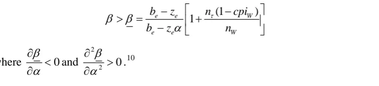
α ∂ < ∂ and 2 2 0 β α ∂ > ∂ . 10
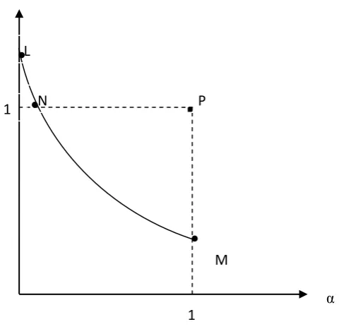
Equation (13) is represented schematically in Figure 2. In this diagram the values of α lies within the range α∈
[ ]
0,1 and whilst in principle β can take any value, we confine our attention to positive values and are particularly interested in range β ∈[ ]
0,1 .11 Combinationsof α and β above the zero employment change locus, LNM, generate an increase in
employment, whilst those below this line are associated with employment decline. We know from the analysis earlier in this sub-section, that where α = β = 1 the employment change associated with the fiscal expansion is positive. This is given as point P in Figure 2. The zero employment change (ZEC) locus therefore lies below this point but its exact position depends upon the general equilibrium elasticities nw, nτ and cpiw, together with the bargaining and migration parameters be and we.
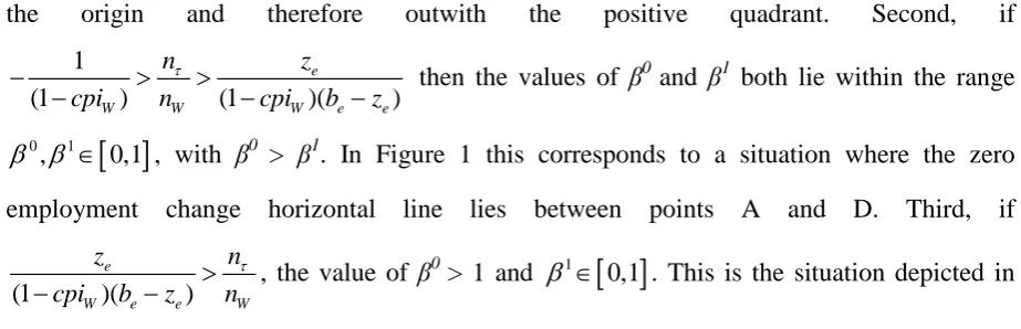
There are three interesting general cases, which are specified by the value of the ratio of the two general equilibrium employment elasticities, nτ/nW. These general cases can be linked back to Figure 1. The partial derivatives from equation (13) show that the relationship between
β and α along the ZEC locus in Figure 2 is downward sloping and convex. We are interested additionally in the values of β at the end points, that is where α is zero and one, identified as β0 and β1respectively.
First, if 1
(1 )
W W
n
n cpi
τ ≥ −
[image:15.595.75.464.71.160.2]− then employment increases for all positive values of α and β. In
Figure 1, this corresponds to the situation where the horizontal zero employment line, there shown as GMHJK, lies above the point A. In this case the ZEC locus in Figure 2 lies below
10. The actual values are given by e
e e z b z β β α α ∂ =
∂ − and
2 2 2 2 2 ( ) e e e z b z β β α α ∂ = ∂ − .
the origin and therefore outwith the positive quadrant. Second, if 1
(1 ) (1 )( )
e
W W W e e
n z
cpi n cpi b z
τ
− > >
− − − then the values of β
0
and β1 both lie within the range
[ ]
0 1
, 0,1
β β ∈ , with β0 > β1. In Figure 1 this corresponds to a situation where the zero employment change horizontal line lies between points A and D. Third, if
(1 )( )
e
W e e W
z n
cpi b z n
τ >
− − , the value of β
0
[image:16.595.68.530.73.222.2]> 1 and β ∈1
[ ]
0,1 . This is the situation depicted in Figure 2 where the point L is (0, β0) and M is (1, β1). It also corresponds to the outcome represented in Figure 1, where the GMHJK zero employment change line lies between points D and L.3.2 National Wage Bargaining with Regional Flow Migration Equilibrium
In Section 3.1 we have adopted a local real wage bargaining framework for the determination of the regional wage. However, it is often argued that within the UK the regional wage is set at the national level, either by national bargaining or through company-wide wage setting in multi-plant firms. Expressed in total differentials, equation (5) can be replaced by dW =0. Doing the appropriate substitutions in this case generates the results: dcpi=0, dn=n dτ τ >0,
0
dw= −dτ < and (1 ) 0 1
e
de d iff
zβ τ β
−
= − > < . Employment increases. However the real
wage falls by the full amount of the tax change and employment rate rises for values of β less than unity, in order to satisfy the zero net migration constraint. Essentially, with national wage bargaining there are the familiar expansionary demand effects associated with the shift from private consumption to public expenditure, but no adverse competitiveness impacts.
In terms of Figure 1, bargaining function, B0, can be replaced by a zero-change pre-tax nominal wage line, which is the de axis, line 0L. The equilibrium is now where the zero net migration function cuts the de axis. The equilibrium value of dW is clearly zero but as argues
above, the change in de depends on the value of β. Where β <1, the equilibrium lies to the right of the origin so that de > 0. Where β >1, the equilibrium is to the left of the origin and de
3.3 Regional Real Wage Bargaining and Zero Labour Mobility Equilibria
Inter-regional migration has played a central role in the analysis up to this point. However, UK regional problems are often linked to restrictions in geographic labour mobility.12 It is therefore valuable to investigate the consequences of imposing the limiting case of zero labour mobility.
The implication of removing migration from the analysis is that equation (1) is dropped. The nominal wage, employment (and employment rate) are now determined by the interaction of the real wage bargaining function, derived as equation (7) in Section 3.1 and the labour demand function, equation (4), suitably expressed in total differentials as:
0, 0
W
W W
n dn
dW d n n
n n
τ
τ τ
= − ≤ ≥ (14)
The model is calibrated with the initial labour force set to unity, which implies that with no migration de = dn. This result, together with equations (7) and (14), generates the expression for the change in total employment and the employment rate as:
(1 ) (1 )
1
W W
W W e
cpi
de dn d
cpi b
τ
η αβ η τ
η
− + −
= =
− − (15)
where de>0iff ητ(1−cpiW)> −ηW(1−αβ);
( ) ( ) ( )
, , 0
de de de
τ
η α β
∂ ∂ ∂ >
∂ ∂ ∂ ; ( ) 0 W de cpi ∂ < ∂ .and ( )
0 e 1
W
de
iff bητ αβ η
∂ > + >
∂ .
13
12 This is not to support the supposed conflict between the bargained real wage function and the zero net migration condition implied in Blanchflower and Oswald (1994). But Blanchflower and Oswald’s (1994)
objection to the Harris-Todaro (1970) function on which the net migration function of Layard et al, (1991) is
based, does reflect the conventional wisdom in the UK that labour mobility is very low, even though Layard et
al’s analysis is based on econometrically estimated net migration functions.
Equation (15) again shows the net employment impact to be the result of two opposing forces. These are the conventional expansionary balanced-budget
13 The actual values are given by: ( ) 1 , ( ) ,
1 1
W W
W W e W W e
cpi
de de
cpi b cpi b
τ
βη
η η α η
− ∂ = ∂ = − ∂ − − ∂ − − ( ) ( ) , 1 1 W
W W e W W W e
de de
cpi b cpi cpi b
τ
αη η
β η η
∂ = − ∂ = −
∂ − − ∂ − − and 2
(1 )( 1 )
( )
(1 )
W e
W W W e
cpi b de cpi b τ η αβ η η − + − ∂ =
∂ − − . For
high values of αβ the change in employment is negatively related to the elasticity of demand for labour. This is
demand shock and the negative competitiveness effects. Employment change will be greater the more inelastic the labour demand function, the higher the valuation of public expenditure, the greater the extent to which this valuation is incorporated into the bargaining function and the lower the feedback of wage changes to the cpi.
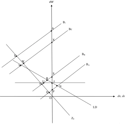
The comparison of the impact of the fiscal expansion under zero labour mobility and flow equilibrium migration can be studies more fully using Figure 3, which adopts the same notation as in Figure 1. Under flow equilibrium migration the equilibrium is at the intersection of the bargained real wage and zero net migration functions whilst under zero labour mobility it is at the intersection of the bargained real wage and the labour demand function.
In interpreting the results from Figure 3, recall that whilst under the zero mobility case changes in employment and the employment rate are identical, under flow migration, this is no longer the case. Because the labour force is endogenous under flow migration, it is quite possible for the employment rate to fall but the absolute level of employment to rise. However, in order to compare the employment change in the two cases it is sufficient to compare the change in the nominal wage. From equation (14) it is clear that for the same fiscal injection, the outcome with the lowest change in nominal wage will have the highest increase in employment.
In Figure 3, the labour demand function is represented by the curve LD. This cuts the de and dW axes with the positive values n dτ τ and
W
n d n
τ τ
− respectively. Note that the labour demand
curve cuts the dW axis at point J, the value for the change in nominal wage which generates zero employment change in the model with migration. The correspondingly points at which the bargaining functions cut the de and dW axis are (1 )
e
d bαβ τ −
− (a negative value) and
(1 )
(1 cpiW)d
αβ τ
−
− respectively. BA, BB and BC correspond to different values of the combined parameter αβ, which represents the value of the public expenditure incorporated into the
bargaining function. As αβ falls the bargaining function makes a parallel upward shift. Note
Begin with the relatively high value of αβ represented by BA. The equilibrium for the zero labour mobility case is at N, representing an increase in employment and the nominal wage. However, recall from the discussion in Section 3 that where the parameters lie in the range 1 ≥
α,β ≥ 0, the equilibrium with flow migration lies within the triangle AD0. This implies that
with these parameter restrictions, the equilibrium must be located on the line segment PQ and the corresponding change in the nominal wage must be lower than in the zero labour mobility case. Therefore where the employment change under zero labour mobility is positive, the long-run employment increase with flow migration will be higher. Essentially, if the employment rate increases where there is zero labour mobility, the introduction of migration will lead to in-migration, reducing the nominal wage and increasing employment.
The bargaining function BBillustrates a situation where the value αβ is slightly lower. In this case the equilibrium with zero labour mobility is at R, and employment falls. However, in this case, given that the regional flow migration equilibrium position lies on the line segment TS,
the change in employment could be positive or negative, depending on the value of β.
Moreover, with a negative employment change that value could be greater or less than under zero labour mobility.
Assign the value of αβ that corresponds to the bargaining function BB the value Β (<1), so that in this case, αβ = Β. Point T identifies the equilibrium where β =1,α = Β. Alternatively, point S is where β = Β,α =1. This implies that for relatively high values of β the equilibrium under flow migration lies in the range TU and employment change will be positive:
W
n
dW d
n τ τ
< − . With lower values of β leading to an equilibrium in the range UR the
employment change is negative but has a smaller absolute value than with zero labour
mobility. However with values of β that generate equilibria in the range RS, the employment
reduction with zero labour mobility is less than with flow migration. In this case the low value
With bargaining function BC the value of αβ is further reduced. In this case, the zero labour mobility equilibrium is at V, whilst the regional flow migration equilibria lie within the range WX. In this case employment falls for both closures but the decline under flow migration is greater than with for zero labour mobility because the increase in the nominal wage is greater.
4. COMPUTABLE GENERAL EQUILIBRIUM MODELLING WITH A SCOTTISH MODEL
4.1 Regional Computable General Equilibrium Modelling
General equilibrium numerical simulation augments the analysis by providing a more extensive treatment. The use of CGE models to identify the likely impacts of fiscal innovations is well established both at the national (e.g. Shoven and Whalley, 1992) and regional (e.g. Hirte, 1998; Jones and Whalley, 1988; Morgan et al. 1989) levels.14 In this case, CGE analysis is particularly appropriate for a number of reasons. First, it is clear from the analysis in the previous subsections that the key general equilibrium elasticities determine not just the quantitative but also the qualitative characteristics of the balanced fiscal expansion equilibrium. Such elasticities are difficult to determine without general equilibrium simulation. Second, the analytical model gives only long-run equilibrium values: it tells us nothing about the time path to this equilibrium. Third, a CGE model gives the change in values for a wide range of aggregate variables and allows for sectoral disaggregation.
However, one problem in tackling this issue through simulation is that existing UK empirical work on regional wage and migration functions offers no direct evidence on the parameter values α and β since the UK has no experience of a local income tax. Furthermore, there is no consensus on the nature of long-run tax effects on the bargained real wage even at the national level (Church et al, 1993), and the relevance of such evidence to the present regional context is, in any case, questionable. Further, whilst there is evidence from other countries on values of α and β, the results are extremely mixed and appear to depend on the composition of public expenditures. (Bartik, 1992; Cebula, 2002; Dahlberg and Fredriksson, 2001; Dalenberg and Partridge, 1995; Day, 1992; Fisher, 1997; Feld and Kirchgassner, 2002; Gabe and Bell, 2004;
Helms, 1985; Mofidi and Stone, 1990; Wallace, 1993).
The available empirical evidence therefore does not allow us to tie down the values of α and β at all precisely. However, our reading of the literature is that the tendency of conventional neoclassical analysis to ignore the potentially beneficial impacts of regional public expenditures is rejected by those studies that provide a balanced treatment of tax and expenditure effects (e.g. Gabe and Bell, 2004). Furthermore, the suggestion that the composition of expenditures influences the values of key parameters implies that they are sensitive to policy choices.
Against this background, there is a strong case for progressing the analysis via numerical simulation as long as the sensitivity of the results to the values taken for α and β is a central feature. However, qualitative and quantitative results concerning the change in the level of economic activity associated with a balanced budget expansion typically depend upon the entire empirical general equilibrium system, as well as the values of α and β. Using a regional CGE model, we are able to estimate the likely size of these effects via simulation over a plausible range of values for α and β. This allows us to identify the combinations of these parameter values associated with positive and negative balanced-budget employment multipliers.
4.2 AMOS: A macro-micro model of Scotland
AMOS is a CGE modelling framework parameterised on data from Scotland.15 Essentially, it is a fully specified, empirical implementation of the skeletal theoretical model developed in Sections 2 and 3. It has three domestic transactor groups, namely the personal sector, corporations and government; and four major components of final demand: consumption, investment, government expenditure and exports. There are eleven commodities/activities but in the simulation results reported in Tables 1, 2 and 3, these are aggregated into three broad industrial groups: manufacturing, non-manufacturing traded and a sheltered sector.16
15 AMOS is an acronym for A Macro-micro Model Of Scotland. The model is calibrated using a Social
Accounting Matrix based around the 2004 Scottish Input-Output Tables (Scottish Government 2007).
Consumption and investment decisions reflect intertemporal optimization with perfect foresight (Lecca et al, 2010). The detailed treatment is given in Appendix 2. Real government expenditure is equal to the base year level plus an additional amount that just exhausts the increment to tax revenue raised by the local income tax. This implies that government expenditure becomes dependent on the entire general equilibrium of the system, which is exactly what would happen if the Scottish Variable Rate were to be implemented. The demand for Scottish Rest of the UK (RUK) and Rest of the World (ROW) exports is determined via conventional export demand functions where the price elasticity of demand is set at 2.0. Imports are obtained through an Armington link (Armington, 1969) and therefore relative-price sensitive with trade substitution elasticities of 2.0 (Gibson, 1990).
In all the simulations in this paper we impose a single Scottish labour market characterised by perfect sectoral mobility. All sectors are taken to be perfectly competitive and produce using multi-level CES production functions with elasticities of substitution of 0.3 (Harris, 1989). We do not explicitly model financial flows, our assumption being that Scotland is a price-taker in competitive UK financial markets.
As regards demographic developments, we assume no natural population change but in the default version of the model, the labour force adjusts using the econometrically parameterised regional net migration function reported in Layard et al (1991), augmented to accommodate the amenity effects discussed in Sections 2 and 3. The model starts in long-run equilibrium with zero net migration flow and, in any subsequent period, migration is taken to be positively related to the gap between regional and national real tax-adjusted wages, and negatively related to the gap between national, and regional unemployment rates:
0.08 ln( ) ln( ) 0.06 ln ln(1 ) ln
S R
S R
S R
w w
m u u
cpi cpi
ς β τ
= − − + − − −
(16)
where m is net in-migration as a proportion of the regional population; u is the unemployment rate for Scotland, β is the relative valuation of the public expenditure and the S and R
superscripts stand for Scotland and the Rest of the world, respectively.17
(
)
ln ln( ) ln 1
S
S S
w
= b + 1.33 u +
cpi β τ
−
In the long run, there is an implied zero-net-migration condition that yields estimates of the optimal spatial distribution of population. This is:
(17) where b again is a calibrated parameter. Wage setting is determined by a regional bargained real wage function that embodies the econometrically derived specification given in Layard et al (1991), again augmented by amenity effects:
( )
(
)
ln 0.113ln ln 1
S
S S
w
= c u +
cpi αβ τ
− −
(18)
where α represents the extent to which the amenity effect is reflected in the wage bargain and c is a calibrated parameter.
5. SIMULATION RESULTS
In this section, we use AMOS to conduct simulations to illustrate the long-run effects of the Scottish Variable Rate on the Scottish economy. Given that the model is parameterised on 2004 data we use the 2004 HM Treasure Budget estimate that exercising these fiscal powers would raise £810 million at 2004 prices, which represents a 1.52 percentage point rise in average personal income tax in AMOS.
5.1 Inter-regional migration and regional bargaining
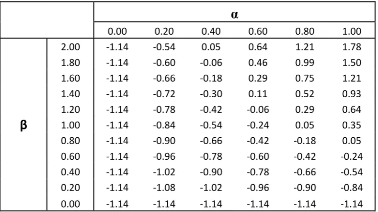
In Table 1 we report the long-run proportionate changes in Scottish employment after the introduction of such a tax for combinations of α and β, where αlies in the range 0 to 1 and β in the range 0 to 2. Figure 4 illustrates these results graphically. These outcomes are consistent
with the analytical results generate in Section 3.4. When the parameters α and β both take a
value of unity, the employment change is positive at 0.68%. Recall that this case produces results that replicate the standard Keynesian balanced budget multiplier, although here the outcome depends on endogenous population and investment effects. Moreover, the level of
employment change is positively related to the values of the parameters α and β. Even a
relatively small reduction in the value of either of these parameters below unity leads to employment falling with a balanced budget fiscal expansion.
A critical point is that once supply-side considerations are included, for a fiscal expansion to have a positive impact on employment, government expenditure must be valued by existing
and potential Scottish residents. Where α = 1, so that the value of the consumption of the public good is fully reflected in the wage bargain, employment falls with a fiscal expansion for
values of β less than 0.76: for α = 0.8, employment falls for values of β less than 0.93.
However, equally, an increase in public expenditure that has a high marginal value for existing and potential Scottish residents will have a depressing aggregate long-run economic impact if these benefits are not incorporated into the wage bargain. In Table 1 results are shown for simulations where the maximum value of β is 2; that is, where marginal valuation of public
expenditure is twice that of private expenditure. Even in this case, for values of α less than 0.32, employment falls with a fiscal expansion. Where β equals unity, so that actual and potential Scottish residents are indifferent between marginal increases in private consumption
and public expenditure, if α takes a value below 0.74, employment falls. This is represented by
point H in Figure 1 and N in Figure 2. Again, where β = 0.8, employment falls for any value of
α below 0.95. Note that where the labour market is perfectly competitive (α = 0), employment always falls with the range of values for β given here.
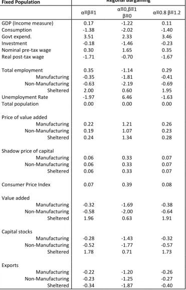
In Table 2 we give the proportionate changes in a more comprehensive set of economic
variables for four particular combinations of α and β. This allows a fuller investigation of the
economic forces at work in each of these cases. In the first column we report results from
simu latio n s wh ere α = β = 1 . Th is is th e situation that corresponds to the conventional Keynesian balanced budget multiplier, albeit with endogenous investment and population.
each sector, output, employment and capital stock vary by the same proportionate amount.18 The demand disturbance comes through the replacement of a proportion of private consumption expenditure by public expenditure.
As argued in Sections 2 and 3, this has a general expansionary impact on the regional economy. The 3.77% increase in government expenditure produces an increase in Scottish GDP of 0.47% and in employment and population of 0.68%. However, the adjustment in consumption and government demand has an uneven effect across sectors. Value added in the sheltered sector, which is most strongly represented in government expenditure, increases by 2.26%. In the other two sectors value added falls, but by a relatively small amount, -0.02%, in manufacturing and by -0.26% in non-manufacturing traded.
The second column gives the simulation results with the parameter values α = 0 and β = 1.
This simulation corresponds to the equilibrium represented by point D in Figure 1. Here private consumption and public expenditure are equally valued at the margin but this is not reflected in the bargained wage. We know from the previous analysis that with this combination of parameter values the nominal pre-tax wage and the unemployment rate rise. In this case the figures are 2.39% and 1.35% respectively. This generates a negative competitive effect. Value-added prices rise by 1.76% in Manufacturing, 1.56% in Non-Manufacturing Traded and by 1.94% in the Sheltered sector. Exports therefore fall in all sectors and this swamps any expansionary impacts generated by the other final demand shifts. Scottish GDP, total employment and population decline by 1.97%, 1.95% and 1.71% respectively, with activity falling in all sectors, though particularly the non-sheltered sectors. The decline in Scottish real income is associated with a smaller rise in the endogenous public expenditure, which increases by 1.69% with these parameter values.
The results in the third column are derived where β = 0. This corresponds to a situation where
the amenity funded by the tax revenue has no value to existing or potential Scottish residents.
The outcome is independent of the value of α and corresponds to point A in Figure 1. In this
simulation there is no change in the post-tax real consumption wage or the unemployment rate. The nominal pre-tax wage increases by 2.60%, the full extent of the tax plus the rise in the consumer price index. This results in an increase in value added prices in all sectors with a corresponding reduction in exports. The impact on individual sectors is qualitatively similar to
the case where α = 0 and β = 1, except that the results here are more extreme. The percentage
change in government expenditure is now 1.52% and Scottish GDP falls by 2.18%, with employment and population both decline by 2.17%. This is the "worst-case" scenario for the Scottish Variable Rate.
The final simulation, reported in column four, adopts the parameter values α = 0.80, β = 1.20
and represents an equilibrium lying in the area 0HML in Figure 1 where β > 1 and both
employment and the nominal pre-tax wage increase. The 0.05% rise in the pre-tax nominal wage following the introduction of the Scottish Variable Rate reduces exports in all sectors. However, the other expansionary fiscal demand impacts produce a more than offsetting effect on overall Scottish aggregate activity. Therefore, although there are small employment falls in the manufacturing and non-manufacturing traded sectors of 0.08% and 0.35%, employment in the sheltered sector rises by 2.20% producing an aggregate increase in GDP, total employment and population of 0.42%, 0.62% and 0.67% respectively.
5.2 Inter-regional migration and national bargaining
The results presented in the first column of Table 2 also give the outcome where there is
national bargaining with the value of β = 1. The nominal wage and unemployment rate remain
unchanged, and population rises by 0.68%. There is a positive stimulus to the Scottish economy that corresponds to the conventional Keynesian balanced budget multiplier. For
alternative values of β under national bargaining, the changes in the unemployment rate and
population level do vary so as to maintain the zero net migration requirement. But in the present parameterisation of the model, this has no direct impacts on household expenditure, so
that the change in all other variables is as under column one of Table 2. Where β equals zero,
so that the additional public expenditure has no value to Scottish residents, population rises by
0.42% and the unemployment rate falls by 1.45%. On the other hand, where β = 1.2,
5.3 Zero population mobility and regional bargaining
Table 3 shows the percentage changes in key variables for the fiscal expansion in a model with bargaining and zero population mobility. As discussed in Section 3.3, in this case the migration function is dropped and the bargaining function is affected by the product of the two
parameters: αβ. This composite parameter measures the extent to which the increase in public
expenditure is incorporated into reduced wage claims.
The first column gives results where αβ = 1, which would correspond, inter alia, to the set of
values α = 1, β = 1. In this case the public consumption is valued equally with private
consumption and this is fully reflected in the bargaining function. In Figure 3 this is represented by a position where the bargaining function remains unchanged as a result of the fiscal expansion and still passes through the origin (the BRW function B0 in Figure 1). Here GDP increases by 0.17%, employment by 0.35% and the nominal pre-tax wage by 0.30%. Increased nominal wages lead to higher value added prices and exports fall in all sectors. Value added increases in the Sheltered sector, by 1.96%, but falls in the Manufacturing and Non-Manufacturing sectors by 0.32% and 0.58% respectively.
The simulation results for α = 0.8, β = 1.2 (so that αβ = 0.96) there is again a stimulus to GDP
but here slightly lower with a slightly greater loss in competitiveness. The bargaining function moves upwards with the fiscal expansion to a position such as BA in Figure 3. Finally where αβ = 0, there is a decline in GDP, and employment by 1.22% and 1.14%. This corresponds to the simulations previously where β = 0 or where α = 0, β = 1, and the bargaining function is
given by B1 in Figure 3. In this case there a large reductions in exports in all sectors and although value added in the Sheltered sector rises by 0.63%, it falls in the Manufacturing and Non-Manufacturing Traded sectors by 1.69% and 2%.
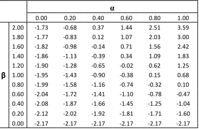
Table 4 gives the percentage change in employment for combinations of the parameters α and
β with zero population mobility. It is instructive to compare these numerical results with
the model incorporating inter-regional migration, reported in Table 1. These results are consistent with the situation represented by bargaining function BAand apply for values of αβ ≥ 0.8.
There is one set of parameters (α = 0.4, β = 1) where the employment change under zero population mobility is negative, but under inter-regional migration it is positive. There is also
one set of parameters, where α = 0.6, β = 1.2, where employment change in both models is negative, but the zero population mobility model has a larger negative value. Both cases are on
the same bargaining function where αβ = 0.72, which corresponds to BB in Figure 3.
In all other case, the employment falls in both models and the fall is greater where there is inter-regional migration. This applies where the value of αβ ≤ 0.64. It corresponds to the bargaining function BC in Figure 3
6. THE ADJUSTMENT PROCESS AND SENSITIVITY
6.1 Time Period of Adjustment
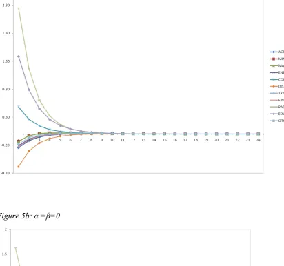
The analysis in the paper deals with long-run equilibria. However, it is also important to consider the adjustment process so as to identify the length of time for equilibrium to be attained and the relevant shorter-run impacts. Figure 5a and 5b plot the period-by-period percentage changes for the Tobin’s q, disaggregated by sector, associated with the introduction of the Scottish Variable Rate. Figure 5a is for the case where α and β are both unity and Figure 5b where both are zero. Note that the adjustment process, which depends on the interaction of migration, consumption and investment decisions, is relatively rapid where the two parameters are both unity but rather protracted for the case in which α and β are both zero. In the first case it it seems that the adjustment is complete something after 10 periods while in the second case takes almost 20 years for the Tobin’s q to achieve constant accumulation rate
expenditure is more concentrated. However, after period 5, the value of Tobin’s q is below its initial value in all sectors due to the depression in economic activity. When α = β = 1, positive investment results occur not only in sheltered sectors but also in Construction. For all the other sectors, although there is a general expansion in economic activity with the introduction of the SVR, there is a long-run reduction in capital stock and therefore disinvestments. Most of these sectors are relatively open to inter-regional and international trade. The rise in the pre-tax bargained nominal wage has adverse competitiveness effects that reduce profit expectations in these sectors.
6.2 Sensitivity Analysis
One criticism of CGE models is that they are not econometrically estimated and that the results might be very sensitive to imposed parameter values. In the existing simulations, the values of the constant elasticity of marginal utility, the CES production substitution elasticities between labour and capital are 0.9 and 0.3. Also the substitution elasticities between locally produced and imported commodities used in production and final demand and the export demand price elasticity take the value 2.0. In this sensitivity exercise, the values of the constant elasticity of marginal utility are selected from the range (0.2 – 1.6), the production substitution elasticities from the range (0.1 - 0.5) and the trade elasticities from the range (0.1 - 4.0).
We assume that all the elasticities have uniform distributions that are symmetric about their means, which are the default point estimates in AMOS. Following Harrison and Vinod (1992), we divide the distribution into 4 equal intervals and since there are 66 elasticities selected, the set of all possible parameter perturbations is 466. However, we adopt a complete randomized factorial design and selected only a subset (1000) of the possible configurations. Each of the 1000 simulations is run for 50 periods.
range of results. Note that, in general, the one standard deviation confidence limits are small and fall over time. This is because in these two cases, migration and investment reduce the price deviations upon which the production and demand elasticities bite. This is particularly apparent in the simulation results reported in Figure 6, where α and β are both unity. From Table 2 it is apparent that in this case extended Input-Output results hold in the long run: there are no relative price changes, so that variation in price elasticities play no role and the confidence range ultimately collapses to a single point (McGregor et al, 1996b). In Figure 7, where (α, β) values are (0.8, 1.2), price changes are still present in the long run so that employment is still sensitive to these parameter values in this case.
7. CONCLUSIONS
In this paper we focus primarily on the potential impact on economic activity of the Scottish Parliament’s exercising its current limited degree of fiscal autonomy through implementing the Scottish Variable Rate. Algebraic and geometric approaches, using a stripped-down regional general equilibrium variant of the Layard et al (1991) model, provide powerful conceptual insights. These include extending the conventional balanced-budget multiplier analysis to accommodate the supply side in a long-run, regional context. Numerical CGE simulation results reinforce and extend this analysis.
However, if the recommendations of the Calman Commission are introduced, the probability that such powers will be used in the future is much increased.
REFERENCES
Armington, P. (1969), "A Theory of Demand for Products Distinguished by Place of Production", IMF Papers, vol. 16, pp. 157-178.
Ashcroft B., Christie, A. and Swales, K. (2006) “Flaws and Myths in the Case for Scottish Fiscal Autonomy”, Fraser of Allander Quarterly Economic Commentary, vol. 13, no. 1, pp. 33-39.
Bartik, T. (1992) “The Effects of State and Local Taxes on Economic Development: A Review of Recent Research,” Economic Development Quarterly, vol. 6, pp.102-110.
Bell D. (2000) ‘The Barnett Formula’, mimeo, Department of Economics, University of Stirling, Stirling.
Bell, D., Dow, S., King, D.and Massie, N. (1996), Financing Devolution, Department of Economics, University of Stirling, Stirling.
Blanchflower, D.G. and Oswald, A. (1994), The Wage Curve, MIT Press, Cambridge Massachussetts.
Blow, L., Hall, J. and Smith S. (1996),"Financing Regional Government in the UK: Some Issues", Fiscal Studies, vol 17, No. 4, pp. 99-120.
Bradley, J., Whelan, K. and Wright, J. (1995), “HERMIN Ireland”, Economic Modelling, 12(3), July, pp. 28-54.
Cebula, R (2002) “Migration and the Tiebout-Tullock Hypothesis Revisited”, Review of Regional Studies, vol. 32, no 1, Spring/ Summer, pp55-62.
Christie, A. and Swales, J.K. (2010), “The Barnett Allocation Mechanism: Formula Plus Influence?”, Regional Studies, vol. 44, pp. 761-775.
Church, K.B., Mitchell, P.R., Smith, P.N. and Wallis, K.F. (1993), "Comparative Properties of Models of the UK Economy", National Institute Economic Review, August, pp. 87-107.
Commission on Scottish Devolution (2009), Serving Scotland Better: Scotland and the United Kingdom in the 21st Century, Final Report, Edinburgh.
Cornes, R. and Sandler, T. (1996), The Theory of Externalities, Public Goods and Club Goods, Cambridge University Press, 2nd Edition.
Cuthbert, J. (1998) ‘The Implications of the Barnett formula’, Saltire Paper No 1, Scottish National Party, Edinburgh.
Dahlberg, M and Fredriksson, p. (2001), “Migration and Local Public Services”, University of Uppsala, Department of Economics, mimeo.
Dalenberg, D. and Partridge, M. (1995), “The Effects of Taxes, Expenditures and Public Infrastructure on Metropolitan Area Employment”, Journal of Regional Science, vol. 35, pp. 617-640.
Day, K.M. (1992), "Interprovincial Migration and Local Public Goods", Canadian Journal of Economics, vol. 25, pp. 123-144.
Ermisch, J. (1995), “Demographic Developments and European Labour Markets”, Scottish Journal of Political Economy, vol. 42, pp. 331-246.
Engel, C. and Rogers, J.H. (1996), "How Wide is the Border", American Economic Review, vol.86, pp. 1112-1125.
Feld, L P and G Kirchgassner (2002) “The Impact of Corporate and Personal Income Taxes on the Location of Firms and on Employment: Some Panel Evidence for the Swiss Cantons, Journal of Public Economics, vol. 87, pp. 129-155.
Fisher, R. (1997), “The Effects of State and Local Public Services on Economic Development”, New England Economic Review, March/April, pp. 53-67.
Gabe, T. M. and Bell K. P. (2004), “Tradeoffs Between Local Taxes and Government Spending As Determinants Of Business Location”, Journal of Regional Science, vol. 44, pp. 21-41.
Gallagher, J. and Hinze, D. (2005) “Financing Options for Devolved Government in the UK”, Discussion Paper 2005-24, Department of Economics, University of Glasgow.
Gibson, H. (1990), "Export Competitiveness and UK Sales of Scottish Manufactures", Paper given at the Scottish Economists Conference, The Burn, Edzell.
Gordon, R H (1983) “An Optimal Taxation Approach to Fiscal Federalism”, Quarterly Journal of Economics, vol 98, pp567-586.
Greenwood, M. J., Hunt, G., Rickman, D.S., and Treyz, G (1991), “Migration, Regional Equilibrium, and the Estimation of Compensating Differentials”, American Economic Review, vol. 81, pp. 1382-90.
Haavelmo, T. (1945), “Multiplier Effects of a Balanced Budget”, Econometrica, vol. 13, pp. 311-318.