D
Demography, Volume 44-Number 2, May 2007: 199–223 199
USING AGE AND SPATIAL FLOW STRUCTURES IN THE
INDIRECT ESTIMATION OF MIGRATION STREAMS*
JAMES RAYMER AND ANDREI ROGERS
This article outlines a formal model-based approach for inferring interregional age-specifi c migration streams in settings where such data are incomplete, inadequate, or unavailable. The esti-mation approach relies heavily on log-linear models, using them to impose some of the regularities exhibited by past age and spatial structures or to combine and borrow information drawn from other sources. The approach is illustrated using data from the 1990 and 2000 U.S. and Mexico censuses.
emographic estimation in countries with inadequate, inaccurate, or incomplete data-reporting systems often must rely on methods that are said to be “indirect.” Such methods utilize inferential techniques that produce estimates of a particular variable by using data that may be only indirectly related to its value. The indirect estimation of fertility and mortality has a long history in demography. A common strategy there has been to combine empirical regularities with other information to fi ll in the missing data. Functional rep-resentations (Heligman and Pollard 1980) and relational reprep-resentations (Brass 1974) of observed age patterns have occupied a central position in such efforts.
A somewhat dated 1983 United Nations manual serves as a useful entry into the vast literature on the topic. Unfortunately, like most of that literature, it ignores migration: “There are other demographic processes affecting the populations of these countries (mi-gration, for example) which are not treated here” (United Nations 1983:1). More recently, a chapter on indirect estimation methods in an important text on formal demography (Pres-ton, Heuveline, and Guillot 2000) also totally ignores migration. Demographic texts that do include topics on migration estimation tend to focus on residual methods (e.g., Rowland 2003; Siegel and Swanson 2004) similar to those presented by Bogue (1969:758–59) over 30 years ago.
The indirect estimation of migration fl ows has a briefer history, in part because the estimation task is more complicated. The age pattern of migrants depends on the directions of migration. To be effective, therefore, a method must somehow integrate the age pattern with the corresponding spatial pattern. Nonetheless, efforts to indirectly estimate migration streams continue (Ahmed and Robinson 1994; Hill 1985; Nair 1985; Schmertmann 1992; Warren and Kraly 1985; Warren and Peck 1980; Willekens 1999; Zaba 1987), notably those attempting to infer international or undocumented fl ows. This article adds to that literature contributing an operational method for estimating age- and origin-destination-specifi c migration fl ows from data on population stocks and auxiliary information. Much of the background for this approach comes from developments in spatial interaction mod-eling made by geographers in the late 1970s and early 1980s (Plane 1981, 1982; Snickars and Weibull 1977; Willekens 1980, 1982, 1983).
Two procedures are outlined, each of which requires a particular data set. One, past migration estimation, requires a complete set of migration fl ow data for one period and regional population stocks or gross migration fl ows for another. This method essentially
“updates” the migration data of a census in order to satisfy the marginal totals obtained or estimated for a later period of interest. If such migration data are not available, then the second method, infant migration estimation, instead uses an inferred migration spatial structure based on the birthplace-specifi c stock of children under 5 years of age at the time of the census.
This article sets out a methodology that allows for such an integration of estimation strategies. Since the problem is to predict the number of migrants by origin, destination, and age, the appropriate model is the log-linear model. It becomes a vehicle for determining whether the distribution of counts presented in the cells of a table matrix can be accounted for by an underlying structure. If the data are incomplete, then the underlying structure is determined by whatever auxiliary data are available, with the parameters of the log-linear model identifying the contributions of the various partial data sets to the predicted migra-tion fl ows.
We begin the article with the description of a general modeling framework for describ-ing and analyzdescrib-ing the age and spatial structures of interregional migration fl ows and show how it can be used to represent a particular pattern of age and spatial profi les. The approach decomposes an observed pattern into multiplicative components and then transforms that mathematical representation of migration into a statistical one by adopting the log-linear modeling framework for analyzing contingency tables. Two applications follow: the fi rst is a discussion of past migration estimation, and the second is a discussion of infant migration estimation. A nine-region representation of migration fl ows in the United States and a four-region representation of migration fl ows in Mexico are used to illustrate the methods.
The results of this study should be of interest to at least two user communities: (1) migration analysts studying mobility patterns in data-poor, less-developed countries, and (2) population researchers faced with the prospective loss of the detailed migration data formerly contained in the “long-form” questionnaire of past U.S. decennial censuses and replaced in the forthcoming 2010 census by the smaller continuous monthly sampling sur-vey called the American Community Sursur-vey.
DESCRIBING AND ESTIMATING THE AGE AND SPATIAL STRUCTURES OF INTERREGIONAL MIGRATION STREAMS
Migration fl ow patterns exhibit strong age and spatial regularities. In a discussion of new “laws” of migration, Tobler (1995:335) argued that “one of the most studied regularities is the age profi le of migrants.” He then focused on spatial patterns of migrants, presenting a table that “shows the correlation between all six U.S. state-to-state tables for the contiguous United States. Thirty-eight percent of the 1985–1990 migration table . . . can be explained by the 1935–1940 table, and 52% of it can be explained by the 1975–1980 table” (p. 336– 37). A deeper analytical examination of this issue appears in a sequence of recent papers of-fering a formal defi nition of what constitutes the age and spatial structures of migration and how they can be represented by a multiplicative log-linear modeling framework (Raymer, Bonaguidi, and Valentini 2006; Rogers, Willekens, and Raymer 2001, 2002, 2003; Rogers, Willekens, Little, and Raymer 2002). This article adds to that research in two ways. First, a multiplicative component model is used to describe and model age-specifi c interregional migration fl ows in the United States and Mexico—two seemingly different situations. And, second, a consistent model-based framework is applied to estimate migration patterns using two types of auxiliary information, past migration and infant migration.
A Multiplicative Component Approach
two-way origin-destination interaction component representing the impacts of physical or social distance between places (those not explained by the overall and main effects). This breakdown is multiplicative, such that
nij = (T)(Oi)(Dj)(ODij), (1)
where nij is an observed fl ow of migration from region i to region j, T is the total number
of migrants (i.e., n++), Oi is the proportion of all migrants leaving from region i (i.e., ni+ / n++), and Dj is the proportion of all migrants moving to region j (i.e., n+j / n++ ). The interac-tion component ODij is defi ned as nij / [(T)(Oi)(Dj)], or the ratio of observed migration to
expected migration (for the case of no interaction). This general type of model is called a multiplicative component model.
Next, consider the representation of age-specifi c migration patterns between these regions. The multiplicative component model for this table is specifi ed as
nijx = (T)(Oi)(Dj)(Ax)(ODij)(OAix)(DAjx)(ODAijx), (2)
where Ax is the proportion of all migrants in age group x. This model is more complicated
because there are now three two-way interaction components and a single three-way in-teraction component between the origin, destination, and age variables. However, the interpretations of the parameters remain relatively simple and follow the same format as presented for the two-way table. That is, the interaction components represent ratios of observed fl ows or marginal totals to expected ones. For example, the destination-age in-teraction (DAjx) component is calculated as n+jx / [(T)(Dj)(Ax)] and represents the ratios of
observed age patterns of in-migration to each region divided by the expected age pattern of in-migration.
The Log-Linear Model
The multiplicative component descriptive model set out in Eq. (2) can be expressed as a saturated log-linear statistical model,
ln(nijx) iO j D
x A
ij OD
ix OA
jx DA
i
= +λ λ +λ +λ +λ +λ +λ +λODAjjx , (3)
where the λs are simply the natural logarithms of the variables appearing in Eq. (2). In multiplicative form, this model is expressed as
nijx iO j D
x A
ij OD
ix OA
jx DA
ijx ODA
=ττ τ τ τ τ τ τ , (4)
where the τs denote the model’s multiplicative parameters or “effects.” We use this form to
be consistent with the multiplicative component model. The saturated model is expressed as (ODA), using the notation set out in Agresti (2002:320). The parameters of the log-linear model can be analyzed by using standard statistical techniques for categorical data analysis to identify key structures in the data.
Reduced forms of the models set out in Eqs. (3) and (4) are called unsaturated models. For example, the model that includes only the main effects of origin, destination, and age is specifi ed as
ˆ ,
nijx iO
j D
x A
=ττ τ τ (5)
main effects is designated as (OD, A) and is specifi ed as nˆijx iO j D
x A
ij OD
=ττ τ τ τ . Such notations are used because these models are hierarchical; that is, for two-way interaction terms, the main effect parameters must be included, and for three-way interaction terms, all the main effects and two-way interactions must be included.
Migration fl ow tables are complicated because they can mix migrants with nonmigrants or intraregional migrants. To remove nonmigrant elements from the analysis, structural zeros can be inserted using an indicator function (Agresti 2002; Willekens 1983). When structural zeros are included in the model, Eq. (5) is called a quasi-independence model.
An offset, a matrix with auxiliary information, can be used to incorporate such informa-tion (as well as structural zeros) to improve the estimainforma-tion procedure. Auxiliary informainforma-tion can be, for example, a historical table of migration fl ows. The log-linear-with-offset model is specifi ed as
ˆ * ,
nijx nijx iO j D
x A
= ττ τ τ (6)
where n*
ijx denotes the auxiliary information (refer to Rogers et al. 2003:60–61). In this case,
the fl ows contained in the offset would be forced to fi t the marginal totals represented by the overall level and main effects of age, origin, and destination.
We use known data in this article to test our ideas. The migrant-only models make the strong assumption that the current marginal totals are known—that is, the overall level of migration, the proportions migrating from and to each region, and the proportions in each age group are given. Our emphasis is on identifying and modeling the age and spatial patterns within these marginal totals. However, some examples are provided in the past migration and infant migration estimation sections that do not make such a strong assump-tion and instead use age-specifi c population stocks at the beginning and end of the interval as the marginal total information to estimate both migrants and nonmigrants. Of course, the marginal totals could also have been modeled independently (Little and Rogers 2007). Furthermore, the modeling framework presented in this paper can be applied to unknown situations. For example, the multiplicative component approach has been applied to project future age-specifi c interregional migration fl ows in Italy (Raymer et al. 2006) and to esti-mate age-specifi c international fl ows between countries in the European Union, Iceland, Norway, and Switzerland during the 2001–2002 period (Raymer forthcoming).
The models in this paper are evaluated using the likelihood ratio statistic, G2,
G2=2 nijx nijx nijx
Σ ln( / ˆ ), (7)
where values closest to zero are associated with “good” fi ts (see, e.g., Agresti 2002). We also use the coeffi cient of determination, R2, when examining particular age-specifi c fl ow estimates. The former is useful for assessing overall fi t in terms of levels; the latter is useful for assessing overall fi t in terms of patterns (or shapes).
APPLICATIONS
The United States
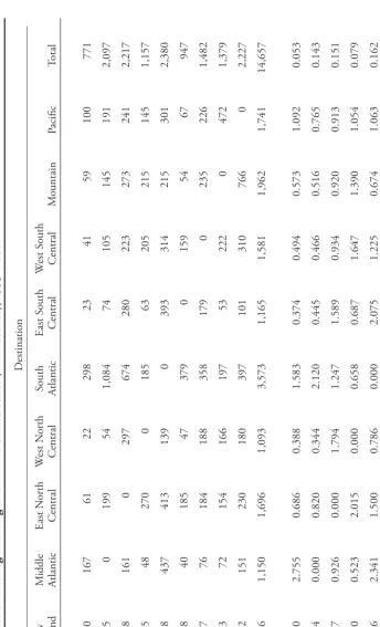
To illustrate the advantages of analyzing migration in terms of multiplicative components, consider the U.S.-born migration fl ows between the nine Census Bureau–defi ned regions (Divisions) during the 1995–2000 time period set out in Panel A of Table 1. Note that non-migrants (i.e., nii) are not included in the table. During this period, 14.6 million U.S.-born
persons over the age of 5 years made an interregional migration. Nearly half of all migrants came from the East North Central, South Atlantic, and Pacifi c regions, and about a quarter of all migrants went to the South Atlantic region. The largest origin-destination-specifi c fl ow was from the Middle Atlantic region to the South Atlantic region.
The multiplicative components corresponding to the migration fl ows discussed above are set out in Panel B of Table 1. Note that the overall component (T) is set out in the total sum (i.e., n++) location of the table, the origin components (Oi) are set out in the row-sum
locations (i.e., ni+), the destination components (Dj) are set out in the column-sum locations
(i.e., n+j), and the origin-destination interaction components (ODij) are set out in the cells
in-side the marginal totals (i.e., nij). For example, consider the Middle Atlantic to South Atlantic
fl ow of 1,084 thousand persons disaggregated into the four multiplicative components:
n25 = (T)(O2)(D5)(OD25)
= ⎛ ⎝ ⎜⎜⎜ ⎜ ⎞ ⎠ ⎟⎟⎟ ⎟⎟ ⎛ ⎝ ⎜⎜⎜ ⎜ ⎞ ⎠ ⎟⎟⎟ ⎟⎟ ++ + ++ + ++ n n n n n n
2 5 225
2 5 n n n n n ++ + ++ + ++
( )
⎛ ⎝ ⎜⎜⎜ ⎜ ⎞ ⎠ ⎟⎟⎟ ⎟⎟ ⎛ ⎝ ⎜⎜⎜ ⎜ ⎞ ⎠ ⎟⎟⎟⎟ ⎟⎟ ⎡ ⎣ ⎢ ⎢ ⎢ ⎢ ⎢ ⎢ ⎢ ⎤ ⎦ ⎥ ⎥ ⎥ ⎥ ⎥ ⎥ ⎥ = ⎛ ⎝ ⎜⎜⎜⎜ ⎞⎠⎟⎟⎟⎟ ( , ) , , , , 14 657 2 09714 657
3 573 14 657
⎛⎛ ⎝
⎜⎜⎜⎜ ⎞⎠⎟⎟⎟⎟⎛⎝⎜⎜⎜⎜1 084511, ⎞⎠⎟⎟⎟⎟ = (14,657)(0.143)(0.244)(2.120)
= 1,084,
where the subscripts 2 and 5 denote the Middle Atlantic and South Atlantic regions, respectively. The interpretations of these components are relatively simple. The overall component is the reported total number of U.S.-born interregional migrants aged 5 years and over; 14.6 million persons made an interregional move between 1995 and 2000. The origin component represents the shares of all migrants from each region: 14%of all mi-grants originated in the Middle Atlantic region. The destination component represents the shares of all migrants to each region: 24% of all migrants moved to the South Atlantic region. And, fi nally, the interaction component represents the ratio of observed migration to expected migration; there were roughly two observed migrants for every one expected migrant. The expected fl ow is based on the marginal total information, for example, (T)(O2)(D5).
T able 1. Th e S patial S tr uctur e of Interr egional M
igration in the U
nited S
tates (in thousands), 1995–2000
D estination ______________________________________________________________________________________________________________________ N ew M iddle East N or th W est N or th South East S outh W est S outh O rigin E ngland A tlantic Central Central A tlantic Central Central M ountain P acifi c T otal A. O bser ve d F lo w s N ew E ngland 0
167 61 22
298 23 41 59
100 771 M iddle A tlantic 245 0 199 54 1,084 74 105 145 191 2,097 East N or th Central 68 161
0 297 674 280 223 273 241
2,217 W est N or th Central 25 48 270 0 185
63 205 215 145
1,157
So
uth
A
tlantic
168 437 413 139
0 393 314 215 301
2,380 East South Central 18 40 185 47 379 0 159 54 67 947 W est South Central 37
76 184 188 358 179
0 235 226
1,482
M
ountain
43
72 154 166 197
53 222 0 472 1,379 Pa ci fi c
92 151 230 180 397 101 310 766
0
2,227
T
otal
696 1,150 1,696 1,093 3,573 1,165 1,581 1,962 1,741
14,657 B. M ultiplicativ e Components N ew E ngland
0.000 2.755 0.686 0.388 1.583 0.374 0.494 0.573 1.092 0.053
M
iddle
A
tlantic
2.464 0.000 0.820 0.344 2.120 0.445 0.466 0.516 0.765 0.143
East
N
or
th
Central
0.647 0.926 0.000 1.794 1.247 1.589 0.934 0.920 0.913 0.151
W est N or th Central
0.460 0.523 2.015 0.000 0.658 0.687 1.647 1.390 1.054 0.079
So
uth
A
tlantic
1.486 2.341 1.500 0.786 0.000 2.075 1.225 0.674 1.063 0.162
East
South
Central
0.393 0.532 1.688 0.664 1.641 0.000 1.554 0.425 0.592 0.065
W
est
South
Central
0.519 0.652 1.071 1.704 0.992 1.516 0.000 1.185 1.281 0.101
M
ountain
0.653 0.662 0.967 1.612 0.587 0.481 1.495 0.000 2.883 0.094
Pa
ci
fi
c
0.873 0.862 0.892 1.082 0.732 0.570 1.291 2.570 0.000 0.152
T
otal
0.047 0.078 0.116 0.075 0.244 0.080 0.108 0.134 0.119
The extension of the above analysis to include age is straightforward. The age groups used in this article start with 5–9 years and end with 85+ years and are measured at the time of the census. There are 17 age groups total. The age main effect component de-scribes the age composition of all migrants in the multiregional system. The origin-age interaction components can be used to identify important differences between age-specifi c out-migration levels from each region and the overall age profi le of migration found in the corresponding expected fl ows (i.e., (T)(Oi)(Ax)). The same is true for the destination-age
interaction components, but with a focus on the differences between age-specifi c in-migra-tion levels to each region and their corresponding expected fl ows (i.e., (T)(Dj)(Ax)).
The origin-age and destination-age interaction components are useful for identifying relative differences found in age patterns of in-migration and out-migration, respectively. For example, in examining the origin-age components (not shown for space reasons; see Figure 3 for example), we found particularly high propensities of young adult migration from the New England, Middle Atlantic, East North Central, and West North Central re-gions. The opposite was true for young adults migrating from the South Atlantic and Pa-cifi c regions. Not surprisingly, out-migration from the New England, Middle Atlantic, and East North Central regions contained age profi les with higher than expected levels around retirement years. The same was true for migration to the South Atlantic and Mountain regions found in the destination-age interaction components (also not shown; see Figure 3 for example).
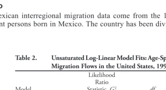
Finally, we compare unsaturated log-linear models to analyze underlying structures in the U.S. migration data. All models include structural zeros to remove nonmigrants from the predictions, and the results, set out in Table 2, are compared using the likelihood ratio statistic. The most obvious fi nding is that the origin-destination interaction term is very important for accurately predicting the age-specifi c migration fl ows. Most of the fl ows do not contain a large retirement peak or major deviations from the overall age profi le of migration. However, the fi ts are slightly improved when the origin-age or destination-age interactions (with the latter doing a better job) are included. Of course, to capture different age profi les found in some of the fl ows, such as those with retirement peaks, origin-age or destination-age interactions have to be included.
Mexico
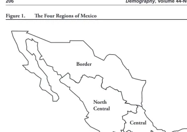
[image:8.612.112.380.509.654.2]The Mexican interregional migration data come from the 1990 and 2000 censuses and represent persons born in Mexico. The country has been divided into four regions on the
Table 2. Unsaturated Log-Linear Model Fits: Age-Specifi c Interregional Migration Flows in the United States, 1995–2000
Likelihood Ratio
Model Statistic, G2 df G2 / df
basis of economics and history (see Figure 1). The Border region has the most formal employment. The North Central region is an area of medium-level development, with an economy focused on manufacturing and export agriculture. The Central region, formerly the most dynamic area in Mexico, remains the country’s fi nancial and political hub, with Mexico City, the capital, as its center. The South region, historically the country’s poorest, currently has an economy based on tourism and petroleum.
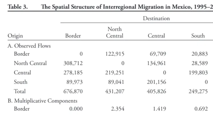
The aggregate migration fl ows between the Border, North Central, Central, and South regions during the 1995–2000 period are set out in Panel A of Table 3, and the correspond-ing multiplicative components are presented in Panel B. Durcorrespond-ing the 1995–2000 period, 1.76 million persons over the age of 5 years (in the year 2000) made an interregional migration in Mexico, with 40% coming from the Central region. The Border region received nearly the same number of migrants. The largest origin-destination-specifi c fl ow was the North Central–Border fl ow. This fl ow had an origin-destination association of 1.7. Other fl ows that exhibited high levels of association (i.e., values greater than 1.5) were the Border– North Central, Central-South, and the South-Central fl ows. In all of these instances, the regions share a border.
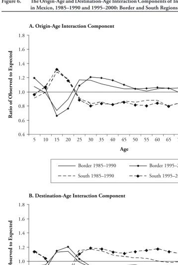
[image:9.612.47.425.75.342.2]Some interesting regional patterns were found in the origin-age and destination-age patterns (again, not shown for space reasons; see Figure 6 for examples). For example, children exhibited higher than expected levels of migration from the Border region. Young adults had higher than expected levels of migration from the South region, whereas from the Border region, the fl ows were lower than expected. Persons older than 25 years were less likely to leave the South, whereas persons aged 30–44 were more likely to leave the Border region. And the elderly were more likely to leave the North Central region. As for the destination-age interaction components, young adults exhibited higher than expected levels of migration to the Border and Central regions. Elderly migrants clearly Figure 1. Th e Four Regions of Mexico
North Central Border
Central
preferred the Central region (home to the capital, Mexico City, and its healthcare facili-ties) to other regions.
A log-linear analysis was also carried out for the Mexican fl ow data. Again, the origin-destination interaction term was found to be very important for accurately pre-dicting the age-specifi c migration fl ows. Most of the age-specifi c regional fl ows did not deviate much from the overall age profi le of migration. However, the fi ts were slightly improved when the origin-age or destination-age interactions were included (with the lat-ter doing a betlat-ter job).
PAST MIGRATION ESTIMATION
The 1995–2000 age-specifi c interregional migration patterns in the United States and in Mexico are estimated in this section, using some of the structures found in the previous census. In particular, the log-linear-with-offset model (i.e., Eq. (6)) is applied to estimate the 1995–2000 age-specifi c interregional migration fl ows. The offset in this case is the matrix of observed 1985–1990 age-specifi c interregional migration fl ows. Depending on the available data, the estimation can focus on (1) migrants or on (2) both migrants and nonmigrants. The fi rst implies that the aggregate numbers of persons in-migrating and out-migrating for each region are known, whereas the second implies that only the beginning and ending regional population stocks are known (a more common situation). For the second case, T denotes the overall population size of persons aged 5 years and older, Oi denotes the proportion of the population residing in a region at the beginning of
the interval, Dj denotes the proportion of the population residing in a region at the end of
the interval, and Ax denotes the proportions of the total population in each age group x.
[image:10.612.60.432.95.296.2]The main concern with modeling both migrants and nonmigrants is the tendency of non-migrants to dominate the results. During the 1985–1990 and 1995–2000 periods, about 93% of the U.S.-born populations and about 98% of the Mexican-born populations were nonmigrants. For direct estimation modeling, this means that any substantial changes in the nonmigrant origin-destination interaction components will have a sizable impact on the predicted fl ows of migration. To demonstrate the implications for the U.S. and Mexico Table 3. Th e Spatial Structure of Interregional Migration in Mexico, 1995–2000
Destination
______________________________________________________________________
North
Origin Border Central Central South Total
A. Observed Flows
Border 0 122,915 69,709 20,883 213,507 North Central 308,712 0 134,961 28,589 472,262 Central 278,185 219,251 0 199,803 697,239 South 89,973 89,041 201,156 0 380,170 Total 676,870 431,207 405,826 249,275 1,763,178
B. Multiplicative Components
Border 0.000 2.354 1.419 0.692 0.121
North Central 1.703 0.000 1.242 0.428 0.268
Central 1.039 1.286 0.000 2.027 0.395
South 0.616 0.958 2.299 0.000 0.216
Total 0.384 0.245 0.230 0.141 1,763,178
migration estimations, we used two offsets to estimate the 1995–2000 age-specifi c inter-regional migration fl ows: one that included only migrants and another that included both migrants and nonmigrants.
The United States
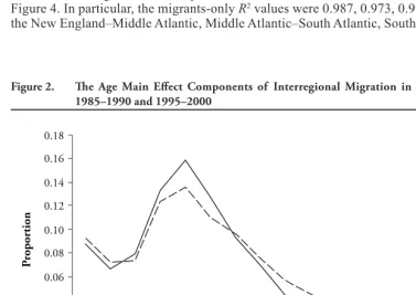
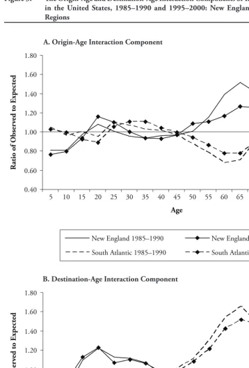
The age and spatial structures of U.S. interregional migration have exhibited stability over time. The age main effect components for the 1985–1990 and 1995–2000 periods are set out in Figure 2. The main differences between the two periods are that the labor force peak became slightly wider in the later period and that the retirement peak disap-peared entirely. New England’s and South Atlantic’s origin-age and destination-age interaction components have been set out in Figure 3 for the two migration periods as a another example of stability over time. Here, the most noticeable differences were found in the retirement years, where the patterns of the 1995–2000 period were less extreme than in the 1985–1990 period. Overall, the comparisons of the age and spatial structures of migration between the two periods show continuity over time and suggest that a model relying on the 1990 census data to estimate the 1995–2000 migration patterns should perform well.
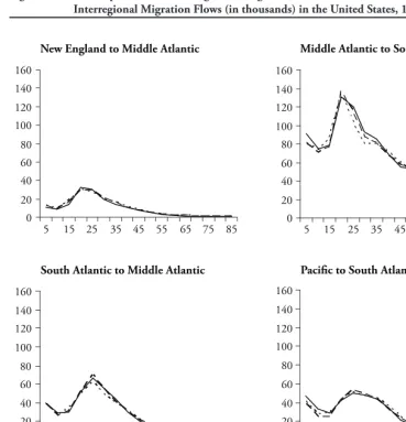
[image:11.612.49.426.380.646.2]The log-linear-with-offset model was applied to estimate the 1995–2000 age-specifi c interregional migration fl ows by “borrowing” the two-way and three-way associations found in the migration data captured in the previous census. Both the “migrants only” and “with nonmigrants” models performed well, as illustrated with some selected fl ows in Figure 4. In particular, the migrants-only R2 values were 0.987, 0.973, 0.994, and 0.971 for the New England–Middle Atlantic, Middle Atlantic–South Atlantic, South Atlantic–Middle
Figure 2. Th e Age Main Eff ect Components of Interregional Migration in the United States, 1985–1990 and 1995–2000
0.00 0.02 0.04 0.06 0.08 0.10 0.12 0.14 0.16 0.18
5 10 15 20 25 30 35 40 45 50 55 60 65 70 75 80 85+
Age
P
ropor
tion
Figure 3. Th e Origin-Age and Destination-Age Interaction Components of Interregional Migration in the United States, 1985–1990 and 1995–2000: New England and South Atlantic Regions
0.40 0.60 0.80 1.00 1.20 1.40 1.60 1.80
5 10 15 20 25 30 35 40 45 50 55 60 65 70 75 80 85+
Age
R
atio of O
bser
ved to E
xpected
New England 1985–1990 New England 1995–2000
0.40 0.60 0.80 1.00 1.20 1.40 1.60 1.80
5 10 15 20 25 30 35 40 45 50 55 60 65 70 75 80 85+
Age
R
atio of O
bser
ved to E
xpected
South Atlantic 1985–1990 South Atlantic 1995–2000
A. Origin-Age Interaction Component
Atlantic, and Pacifi c–South Atlantic fl ows, respectively. For the migrants and nonmigrants model, the R2 values were 0.971, 0.958, 0.986, and 0.984, respectively. The G2 statistics, calculated for these fl ows, correspond with the R2 patterns. Note that these fl ows were selected because of their different age-specifi c shapes. The South Atlantic–Middle Atlantic fl ow has a relatively sharp labor force peak in comparison to the relatively fl at-peaked New England–Middle Atlantic fl ow and the wide labor force curved Pacifi c–South Atlantic fl ow. The Middle Atlantic–South Atlantic fl ow is an example of a fl ow with a retirement peak. In terms of overall fi t, the migrant-only model performed better with a G2 of 236,326 versus –425,830 for the migrants and nonmigrants model.
Figure 4. A Comparison of Past Migration Log-Linear Model Predictions: Selected Age-Specifi c Interregional Migration Flows (in thousands) in the United States, 1995–2000
New England to Middle Atlantic
0 20 40 60 80 100 120 140 160
5 15 25 35 45 55 65 75 85
Middle Atlantic to South Atlantic
0 20 40 60 80 100 120 140 160
5 15 25 35 45 55 65 75 85
South Atlantic to Middle Atlantic
0 20 40 60 80 100 120 140 160
5 15 25 35 45 55 65 75 85
Pacific to South Atlantic
0 20 40 60 80 100 120 140 160
5 15 25 35 45 55 65 75 85
Mexico
A comparison of Mexico’s spatial structures of migration over time illustrates some in-teresting patterns (Table 4). The overall level increased by 6%. The share of migration originating in the Border and South regions increased by 8% and 10%, respectively, and decreased by slightly more than 11% in the North Central region. The proportions of mi-grants going to the Border region increased substantially, whereas those going to the North Central and Central regions declined. For the origin-destination associations, the extremes were those corresponding with the South to Border fl ow, which increased by 67%, and the Central to North Central fl ow, which decreased by 17%.
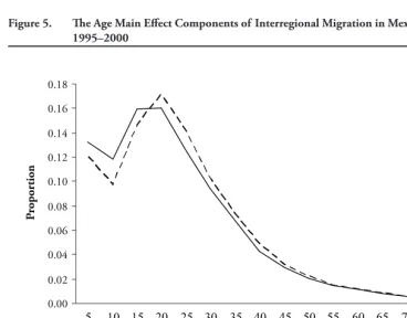
The age main effect components for the 1985–1990 and 1995–2000 periods are set out in Figure 5. The main difference between the two periods is that the labor force peak shifted slightly to the right and that there were slightly lower proportions of young children migrating in the later period. A comparison of origin-age and destination-age interaction components for the Border and South regions during the two migration periods shows strong continuity over time, as illustrated in Figure 6. These age profi les illustrate that young adults were more likely to migrate from the South region and to migrate to the Bor-der region. Not surprisingly, young adults were also less likely to migrate from the BorBor-der region and migrate to the South region. Again, the comparisons of the age and spatial structures of migration between the two periods show general continuity over time and suggest that a model relying on the 1990 census data to estimate the 1995–2000 migration patterns should perform well.
As for the U.S. case study, two offsets were used to estimate the 1995–2000 specifi c interregional migration fl ows in Mexico: one that included only migrants and another that included both migrants and nonmigrants. The model that included both mi-grants and nonmimi-grants overpredicted the number of mimi-grants by 249,000 and had a G2 of –173,004. For the migrants-only model, the G2 was 26,420. A selection of the estimated fl ows is presented in Figure 7. For the migrants-only model, the R2 values were 0.986, 0.996, 0.999, and 0.998 for the Border–North Central, North Central–Border, Central-South, and South-Central fl ows, respectively, and 0.993, 0.996, 0.996, and 0.998, respec-tively, for the migrants and nonmigrants model. Note, for the above fl ows, that the G2 statistics were all substantially closer to zero for the migrants-only model.
INFANT MIGRATION ESTIMATION
[image:14.612.60.433.106.208.2]A new method for indirectly estimating migration patterns was recently put forward by Rogers and Jordan (2004), in which regional birthplace-specifi c population stock data of 0- to 4-year-olds was used to predict age-specifi c interregional patterns of migration in the Table 4. A Comparison of Mexico’s Migration Spatial Structures Over Time: Ratios of 1995–2000
Multiplicative Components to 1985–1990 Multiplicative Components
Destination
_____________________________________________________________________
North
Origin Border Central Central South Total
Border 1.068 1.128 1.273 1.083
North Central 0.857 1.086 1.297 0.886
Central 1.240 0.831 0.942 1.014
South 1.674 1.253 0.876 1.102
Figure 5. Th e Age Main Eff ect Components of Interregional Migration in Mexico, 1985–1990 and 1995–2000
0.00 0.02 0.04 0.06 0.08 0.10 0.12 0.14 0.16 0.18
5 10 15 20 25 30 35 40 45 50 55 60 65 70 75 80 85+ Age
P
ropor
tion
1985–1990 1995–2000
United States. The fi rst age group was used to capture the interregional patterns (not the levels) of the fi ve-year interval migration question. That is, if a child is living in a differ-ent place than his or her place of birth, that child must have migrated at least once during the past fi ve years. The same cannot be said for other age groups. And the reason why the migration pattern of a single age group can predict the corresponding patterns for other age groups comes from the age regularities found in observed migration patterns.
Migration propensities differ greatly according to age. Typically, an age-specifi c profi le of migration shows a downward slope from the early childhood age groups to about age 16, is followed by a rise to a peak in the young adult age groups (usually around age 22), and then gradually tapers off to the oldest age groups. This “standard” age profi le of migration can be fully described by using a multi-exponential model migration schedule (Rogers and Castro 1981; Rogers and Little 1994).
The most often used model migration schedule is the seven-parameter version:
Nijx= +a0 a1exp
(
−α1x)
+a2exp{
−α2(
x−μ2)
−exp⎡⎣⎢−λ2(
x−μμ2)
⎤⎦⎥}
, i≠j, (8)where Nijx denotes standardized (to unit area) age profi les of migration from region i to
region j at age group x. The a0, a1, and a2 are level parameters, whereas the α1, α2, μ2, and
Figure 6. Th e Origin-Age and Destination-Age Interaction Components of Interregional Migration in Mexico, 1985–1990 and 1995–2000: Border and South Regions
A. Origin-Age Interaction Component
0.4 0.6 0.8 1.0 1.2 1.4 1.6 1.8
5 10 15 20 25 30 35 40 45 50 55 60 65 70 75 80 85+
Age
R
atio of O
bser
ved to E
xpected
Border 1985–1990 Border 1995–2000
South 1985–1990 South 1995–2000
B. Destination-Age Interaction Component
0.4 0.6 0.8 1.0 1.2 1.4 1.6 1.8
5 10 15 20 25 30 35 40 45 50 55 60 65 70 75 80 85+
Age
R
atio of O
bser
ved to E
Figure 7. A Comparison of Past Migration Log-Linear Model Predictions: Selected Age-Specifi c Interregional Migration Flows (in thousands) in Mexico, 1995–2000
Border to North Central
0 10 20 30 40 50 60 70 80
5 15 25 35 45 55 65 75 85+
North Central to Border
0 10 20 30 40 50 60 70 80
5 15 25 35 45 55 65 75 85+
Central to South
0 10 20 30 40 50 60 70 80
5 15 25 35 45 55 65 75 85+
South to Central
0 10 20 30 40 50 60 70 80
5 15 25 35 45 55 65 75 85+
Observed Migrants only With nonmigrants
United States and Mexico during the 1995–2000 period. The estimated parameters for the United States are
ˆ . . exp . . exp .
Nijx=0 00 0 11+
(
−0 04x)
+0 19{
−0 061(
x−199 24.)
−exp⎣⎢⎡−0 23.(
x−19 24.)
⎤⎦⎥}
.And for Mexico, they are
ˆ . . exp . . exp .
Nijx=0 00 0 18+
(
−0 07x)
+0 22{
−0 066(
x−155 20.)
−exp⎣⎢⎡−0 30.(
x−15 20.)
⎤⎦⎥}
.The log-linear-with-offset model can be thought of as a relational model (Rogers et al. 2003). In this situation, the offset is the collection of 0- to 4-year-old birthplace-specifi c population stocks. We can specify a log-linear-with-offset model that uses the 0- to 4-year-old birthplace-specifi c population stocks to predict the aggregate patterns (assuming the marginal totals are known):
ˆ * ,
nij nij iO j D
= νν ν (9)
where the offset n*
ij contains the “migration” patterns of those aged 0–4 years at the time
of the census, and effectively serves as a “proxy” for the interaction patterns of the current migration fl ows.
For age-specifi c patterns, the log-linear-with-offset model specifi ed in Eq. (6) can be used. In this case, the offset contains structural zeros in the diagonal and the “migration” patterns of those aged 0–4 years at the time of the census in the off-diagonals. The overall age profi le and aggregate proportions migrating from and to each region are assumed to be known. If instead one has to work with population totals, then one needs to estimate or borrow the aggregate age-specifi c proportions of migrants and nonmigrants. The model used in this case would be
ˆ * ,
nijxz nijxz iO j D
x A
z M
xz AM
= νν ν ν ν ν (10)
where M denotes migrant status (i.e., migrant or nonmigrant status). This specifi cation is required to distinguish between the age profi les of migrants and those of nonmigrants.
The United States
The 0- to 4-year-old “migration” patterns for U.S.-born persons are set out in Table 5. The spatial structure of these “infant” migrants closely resembles that of the period migrants set out earlier in Table 1. The predicted aggregate fl ows from New England and South Atlantic are presented in Figure 8. These predicted fl ows come from the model specifi ed in Eq. (9), but with two alternative offsets being used: (1) migrants only and (2) migrants and nonmigrants. Although both models appear to predict the observed data well, the migrants-only model did considerably better. The likelihood ratio statistics for the two models were 132,799 and –1,632,755, respectively. The corresponding R2 values were 0.985 and 0.955, respectively.
The age-specifi c predictions using the models in Eq. (6) and Eq. (10) also did well, capturing the levels and most of the age profi les. Examples of such predictions are set out in Figure 9. Our illustration applied a single age profi le to estimate all age-specifi c patterns. The age profi le is the same for both the migrants-only and the migrants and non-migrants models. This means that the shapes of some fl ows, such as the retirement migra-tion peak found in the Middle Atlantic to South Atlantic fl ow, were not captured. For the fl ows set out in Figure 9, the R2 values were 0.878, 0.940, 0.967, and 0.948 for the New England–Middle Atlantic, Middle Atlantic–South Atlantic, South Atlantic–Middle Atlantic, and Pacifi c–South Atlantic fl ows, respectively. The corresponding likelihood ratio statistics were lower for the migrants-only model, except for the Pacifi c–South Atlantic fl ow. Over-all, the migrants-only model performed better with an overall G2 of 678,641 versus 890,321 for the migrants and nonmigrants model.
Mexico
T able 5. Th e S patial S tr uctur
e of 0- to 4-Y
ear-O ld B ir thplace-S pecifi c P opulation S
tocks in the U
nited S tates, 2000 D estination ______________________________________________________________________________________________________________________ N ew M iddle East N or th W est N or th South East S outh W est S outh O rigin E ngland A tlantic Central Central A tlantic Central Central M ountain P acifi c T otal A. O bser ve d F lo
ws (in thousands)
N
ew
E
ngland
0
14 5 2
17 2 3 3 6
52 M iddle A tlantic 17 0 19 5 62 6 10 8 14 140 East N or th Central 5 15
0 25 39 24 17 15 18
158 W est N or th Central 2 5 36 0 15 6 19 14 11 106 So uth A tlantic
12 42 44 13
0 35 30 15 28
219 East South Central 2 5 27 6 34 0
18 4 7
103 W est South Central 4
8 20 19 33 15
0 23 26
147
M
ountain
4
8 13 14 17
5 20 0 43 123 Pa ci fi c
8 15 25 18 42 10 32 65
0
214
T
otal
54 111 189 102 258 102 148 147 152
1,264 B. M ultiplicativ e Components N ew E ngland
0.000 3.126 0.678 0.500 1.572 0.464 0.505 0.469 0.915 0.041
M
iddle
A
tlantic
2.824 0.000 0.886 0.472 2.152 0.536 0.594 0.467 0.843 0.111
East
N
or
th
Central
0.708 1.063 0.000 1.918 1.204 1.903 0.929 0.835 0.958 0.125
W est N or th Central
0.471 0.501 2.242 0.000 0.681 0.674 1.502 1.096 0.867 0.084
So
uth
A
tlantic
1.317 2.166 1.344 0.743 0.000 1.974 1.160 0.594 1.063 0.173
East
South
Central
0.506 0.506 1.756 0.735 1.626 0.000 1.450 0.373 0.550 0.082
W
est
South
Central
0.587 0.653 0.920 1.591 1.099 1.231 0.000 1.328 1.438 0.117
M
ountain
0.729 0.733 0.726 1.438 0.657 0.475 1.380 0.000 2.862 0.098
Pa
ci
fi
c
0.882 0.779 0.771 1.017 0.967 0.559 1.277 2.617 0.000 0.170
T
otal
Figure 8. A Comparison of Infant Migration Log-Linear Model Predictions: Interregional Migration Flows (in thousands) From New England and South Atlantic, 1995–2000
From New England
0 100 200 300 400 500
Middle
Atlantic NorthEast Central
West North Central
South
Atlantic SouthEast Central
West South Central
Mountain Pacific
Destination
Observed Migrants only With nonmigrants
From South Atlantic
0 100 200 300 400 500
New England
Middle Atlantic
East South Central
West North Central
East South Central
West South Central
Mountain Pacific
Figure 9. A Comparison of Infant Migration Log-Linear Model Predictions: Selected Age-Specifi c Interregional Migration Flows (in thousands) in the United States, 1995–2000
New England to Middle Atlantic
0 20 40 60 80 100 120 140 160
5 15 25 35 45 55 65 75 85+
Middle Atlantic to South Atlantic
0 20 40 60 80 100 120 140 160
5 15 25 35 45 55 65 75 85+
South Atlantic to Middle Atlantic
0 20 40 60 80 100 120 140 160
5 15 25 35 45 55 65 75 85+
Pacific to South Atlantic
0 20 40 60 80 100 120 140 160
5 15 25 35 45 55 65 75 85+
Observed Migrants only With nonmigrants
migrants-only model once again did a better job, with an overall likelihood ratio statistic of 104,962 versus 150,888 for the migrants and nonmigrants model. The Border–North Central, North Central–Border, Central-South, and South-Central fl ows had R2 values of 0.911, 0.988, 0.929, and 0.933, respectively. The likelihood ratio statistics for these fl ows were lower for all the fl ows in Figure 10, except the South-Central fl ow.
Table 6. Th e Spatial Structure of 0- to 4-Year-Old Birthplace-Specifi c Population Stocks in Mexico, 2000
Destination
______________________________________________________________________
North
Origin Border Central Central South Total
A. Observed Flows
Border 0 26,511 15,549 2,072 44,132
North Central 41,664 0 21,826 4,052 67,542 Central 17,394 31,564 0 28,438 77,396
South 4,147 8,771 25,701 0 38,619
Total 63,205 66,846 63,076 34,562 227,689 B. Multiplicative Components
Border 0.000 2.046 1.272 0.309 0.194
North Central 2.222 0.000 1.166 0.395 0.297
Central 0.810 1.389 0.000 2.421 0.340
South 0.387 0.774 2.402 0.000 0.170
Total 0.278 0.294 0.277 0.152 227,689
and mortality patterns in each region simply shifts the problem to a different potential fl aw—that is, the need to specify the fertility and mortality patterns of migrant populations. Finally, a suggestion was made that a possibly better option would be to use the 5–9 years age group, despite the problem posed by multiple moves. We tried this option and came away with mixed results. We found that when the 5–9 birthplace-specifi c stocks of migrants were used in the offset (i.e., where structural zeros were inserted in the diagonal), the results were indeed somewhat better. But in that alternative, the migration fl ow marginal totals are assumed to be known. However, when 5–9 birthplace-specifi c population stocks were used in the offset (a more common situation), then the predicted fl ows of migrants were overestimated.
DISCUSSION AND CONCLUSION
The age structure of a population is a fundamental concept in demography, one that is normally depicted in the form of an age pyramid. The age structure of migration has also become a fundamental concept, one that can be expressed in the form of a model migra-tion schedule (Rogers and Castro 1981). The spatial structure of an interregional system of origin-destination-specifi c migration streams, however, is a notion that lacks a widely accepted defi nition. In this article, we adopt the defi nition presented in Rogers, Willekens, Little, and Raymer (2002), which draws on the log-linear specifi cation of the spatial inter-action model (Willekens 1983)—a specifi cation that involves a multicomponent breakdown of the matrix of fl ows under study. Such a formulation allows one to capture different fea-tures of a particular spatial structure of migration, with one set of parameters representing the effects of sizes of origin populations, another set representing the corresponding effects of the sizes of destination populations, and still another set representing the strengths of the linkages between these two populations.
Figure 10. A Comparison of Infant Migration Log-Linear Model Predictions: Selected Age-Specifi c Interregional Migration Flows (in thousands) in Mexico, 1995–2000
Border to North Central
0 20 40 60 80
5 15 25 35 45 55 65 75 85+
Age
North Central to Border
0 20 40 60 80
5 15 25 35 45 55 65 75 85+
Age
Central to South
0 20 40 60 80
5 15 25 35 45 55 65 75 85+
Age
South to Central
0 40 60 80
5 15 25 35 45 55 65 75 85+
Age 20
Observed Migrants only With nonmigrants
data because the model then has structural zeroes in the diagonals and avoids the over-whelming infl uence carried by the otherwise nonzero diagonal elements representing the nonmigrants. But the improved accuracy comes at a cost: it needs an estimate of the non-migrant populations that are subtracted from the marginal totals in order to obtain zeroes in the diagonals.
( interactions) between each pair of origins and destinations may be obtained from other auxiliary sources of information, for example, from the migration spatial structure exhib-ited by the under-5 population—one inferred from birthplace-specifi c residence data of that age group in a current census count (Rogers and Jordan 2004). The unique contribu-tion of the log-linear modeling framework for the indirect estimacontribu-tion of migracontribu-tion is its ability to “discipline” these alternative initial estimates by imposing constraints on the es-timated values—constraints that arise from associated historical data, partial data, or even qualitative or judgmental data (Rogers et al. 2003).
As we explained earlier, the U.S. Census Bureau is dropping its long-form question-naire in 2010 and replacing it with a continuous monthly survey called the American Com-munity Survey. This change provides more timely data, but the samples are smaller than have been provided by the decennial census, and the strategy of averaging accumulated samples over time mixes changing migration patterns. Moreover, the migration question re-fers to a one-year time interval instead of the fi ve-year interval used since the 1960 census. For all of these reasons, it may be useful to have at hand a method for complementing or augmenting the collected data with indirect estimates of missing observations, particularly at fi ne levels of age, sex, and spatial disaggregation.
The migration data in less-developed countries, such as Mexico, can be even more problematic, making the log-linear framework presented in this article even more useful. However, certain hurdles posed by, for example, signifi cant differential age misreport-ing and undercountmisreport-ing across regions, will need to be overcome. A National Academy of Sciences report on age-selective underenumeration concluded that, “Although age misre-porting and selective underenumeration will continue to plague demographic studies, the recent evidence suggests that we can do a much better job of adjusting data for misreport-ing errors and of developmisreport-ing techniques for estimatmisreport-ing fertility and mortality that are less sensitive to age reporting errors” (Ewbank 1981:87). The same can be said for the task of estimating migration.
In conclusion, the following observations need to be made. First, the multiplicative component model is a fl exible and powerful framework for analyzing migration fl ows. Second, the log-linear model is an equally fl exible and powerful framework for estimating migration fl ows. Third, estimation of migrant counts alone (with structural zeroes entered in the diagonals) yields more accurate estimates than does the corresponding migrants-plus-nonmigrants estimation procedure. Finally, future work should be directed at the potential improvements provided by the introduction of covariates in the statistical estimation process, for example, the association between the age composition of a population and that of its out-migrants (Little and Rogers 2007).
REFERENCES
Agresti, A. 2002. Categorical Data Analysis. Hoboken, NJ: John Wiley and Sons.
Ahmed, B. and J.G. Robinson. 1994. “Estimates of Emigration of the Foreign-Born Population: 1980–1990.” Technical Working Paper No. 9. Population Division, U.S. Bureau of the Census, Washington, DC.
Bogue, D.J. 1969. Principles of Demography. New York: John Wiley and Sons.
Brass, W. 1974. “Perspectives in Population Prediction: Illustrated by the Statistics of England and Wales.” Journal of the Royal Statistical Society A 137:532–70.
Ewbank, D.C. 1981. Age Misreporting and Age-Selective Underenumeration: Sources, Patterns, and Consequences for Demographic Analysis. Washington, DC: National Academy Press.
Heligman, L. and J.H. Pollard. 1980. “The Age Pattern of Mortality.” Journal of the Institute of Ac-tuaries 107(434):49–80.
Little, J.S. and A. Rogers. 2007. “What Can the Age Composition of a Population Tell Us About the Age Composition of Its Outmigrants?” Population, Space and Place 13:23–39.
Nair, P.S. 1985. “Estimation of Period-Specifi c Gross Migration Flows From Limited Data: Proportional Adjustment Approach.” Demography 22:133–42.
Plane, D.A. 1981. “Estimation of Place-to-Place Migration Flows from Net Migration Totals: A Minimum Information Approach.” International Regional Science Review 6(1):33–51.
———. 1982. “An Information Theoretic Approach to the Estimation of Migration Flows.” Journal of Regional Science 22:441–56.
Preston, S.H., P. Heuveline, and M. Guillot. 2000. Demography: Measuring and Modeling Population Processes. New York: Blackwell.
Raymer, J. Forthcoming. “Obtaining an Overall Picture of Population Movement in the European Union.” In The Estimation of International Migration in Europe: Issues, Models and Assessment,
edited by J. Raymer and F. Willekens. Chicester, United Kingdom: John Wiley and Sons. Raymer, J., A. Bonaguidi, and A. Valentini. 2006. “Describing and Projecting the Age and Spatial
Structures of Interregional Migration in Italy.” Population, Space and Place 12:371–88.
Rogers, A. and L.J. Castro. 1981. “Model Migration Schedules.” RR-81-30, International Institute for Applied Systems Analysis, Laxenburg, Austria.
Rogers, A. and L. Jordan. 2004. “Estimating Migration Flows From Birthplace-Specifi c Population Stocks of Infants.” Geographical Analysis 36(1):38–53.
Rogers, A. and J.S. Little. 1994. “Parameterizing Age Patterns of Demographic Rates With the Mul-tiexponential Model Schedule.” Mathematical Population Studies 4(3):175–94.
Rogers, A., F.J. Willekens, J.S. Little, and J. Raymer. 2002. “Describing Migration Spatial Structure.”
Papers in Regional Science 81:29–48.
Rogers, A., F.J. Willekens and J. Raymer. 2001. “Modeling Interregional Migration Flows: Continuity and Change.” Mathematical Population Studies 9:231–63.
———. 2002. “Capturing the Age and Spatial Structures of Migration.” Environment and Planning A 34:341–59.
———. 2003. “Imposing Age and Spatial Structures on Inadequate Migration-Flow Datasets.” The Professional Geographer 55(1):56–69.
Rogerson, P.A. 1984. “New Directions in the Modelling of Interregional Migration.” Economic Geography 60(2):111–21.
Rowland, D.T. 2003. Demographic Methods and Concepts. Oxford: Oxford University Press. Schmertmann, C.P. 1992. “Estimation of Historical Migration Rates From a Single Census:
Inter-regional Migration in Brazil 1900–1980. Population Studies 46(1):103–20.
Siegel, J.S. and D.A. Swanson, Eds. 2004. The Methods and Materials of Demography. Amsterdam: Elsevier Academic Press.
Snickars, F. and J.W. Weibull. 1977. “A Minimum Information Principle: Theory and Practice.”
Regional Science and Urban Economics 7:137–68.
Tobler, W. 1995. “Migration: Ravenstein, Thornthwaite, and Beyond.” Urban Geography 16: 327–43.
United Nations. 1983. Manual X: Indirect Techniques for Demographic Estimation. New York: Department of International Economic and Social Affairs.
Warren, R. and E.P. Kraly. 1985. “The Elusive Exodus: Emigration From the United States.” Popula-tion Trends and Public Policy Occasional Paper, No. 8. Population Reference Bureau, Washing-ton, DC.
Warren, R. and J.M. Peck. 1980. “Foreign-Born Emigration From the United States: 1960 to 1970.”
Demography 17:71–84.
Willekens, F.J. 1980. “Entropy, Multiproportional Adjustment and the Analysis of Contingency Tables.” Systemi Urbani 2/3:171–201.
———. 1982. “Multidimensional Population Analysis With Incomplete Data.” Pp. 43–111 in
———. 1983. “Log-Linear Modelling of Spatial Interaction.” Papers of the Regional Science Association 52:187–205.
———. 1999. “Modeling Approaches to the Indirect Estimation of Migration Flows: From Entropy to EM.” Mathematical Population Studies 7:239–78.