Psychovisual video coding using wavelet transform

(1)

Psychovisual Video Coding using

Wavelet Transform

by

Dadang Gunawan, Jr., M.Eng.

Department of Electrical and Electronic Engineering

Submitted in fulfillment of the requirements

for the degree of

Doctor of Philosophy

University of Tasmania

(2)

-

TLA_k_z_ s

G-u

N AA A J 1. K 1

V99 9 6-

■

(3)

Statement of Originality

This thesis contains no material which has been accepted for the award of any other

degree or diploma in any tertiary institution. To the best of my knowledge and belief,

the thesis contains no material previously published or written by another person, ex

cept when due reference is made in the text.

(4)

Abstract

Visual communications services are now making a significant impact on modern society. Video conferencing, HDTV and multimedia are just examples where this technology is being used to good effect. Communicating using video signals does, however, require a large volume of data to be transmitted, and even with modern high-bandwidth com-munication links this can be expensive. This requires the implementation of efficient video coding and compression schemes. This thesis investigates both image and video coding compression schemes and aims to develop a scheme with the highest possible performance.

In image coding there are two main types of compression: statistical and psychovisual. This thesis concentrates on the latter, since it is shown that psychovisual techniques, in general, provide greater levels of compression than statistically based methods. The standardised technique for video coding uses psychovisual compression of the coeffi-cients of the discrete cosine transform (DCT). Despite being an international standard for low bit rate video coding the DCT suffers from a number of drawbacks. Firstly, the psychophysical and psychological models of the human visual system (HVS) are based on a multiresolution approach whereas the basis functions of the DCT are fixed in resolution. Secondly the basis functions of the DCT only possess good localisation properties in the frequency domain and not the spatial domain, a characteristic that blurs edges and discontinuities in an image. By contrast the wavelet transform is a mul-tiresolution approach and its basis functions can possess good localisation properties in both the spatial and frequency domains. Furthermore, due to the excellent localisation properties of the wavelet function most of the transform coefficients are practically zero and the use of wavelet transform can be expected to achieve a higher compression ratio than the DCT. This thesis therefore investigates psychovisual transform coding using the wavelet transform instead of the DCT.

(5)

iv

Abstract

Wavelet basis functions are characterised by a number of parameters, often mutually exclusive. These are spatial compactness, orthonormality, regularity or smoothness and symmetry or anti-symmetry. Since orthonormal and biorthonormal wavelet bases have recently been applied in image coding, a discussion on the design of orthonormal and biorthonormal wavelet bases is presented. By including the properties of the HVS sensitivity function into transform coding using the wavelet transform it is shown that certain design parameters can be relaxed in the construction of an effective image coding scheme [1]. Experimentation using orthonormal wavelets in conjunction with the HVS demonstrated that the length of the filter used to implement the orthonormal wavelet decomposition has only a slight effect on the quality of the reconstructed image. The HVS sensitivity function effectively de-emphasizes the high frequency components thereby relaxing the requirement for smooth wavelets which require longer filters and are more expensive computationally [2].

In image analysis and synthesis the properties of symmetrical or linear phase filters are highly desirable. This can only be achieved by using biorthonormal rather than orthonormal wavelets. Often, the decomposition and reconstruction filters associated with biorthonormal wavelets are of different lengths. Due to the HVS smoothing action, high compression ratios can be achieved at a reasonably low computational cost by using short filters or less regular wavelets on the analysis side [2].

The use of the wavelet transform in image coding can be further divided into two ap-proaches, i.e. a conventional approach and a best basis approach. In the conventional approach, the wavelet basis functions are recursively applied to successively coarser approximation signals, in order to extract the difference in information between con-secutive resolutions. The best basis approach involves transforming the image into a set of over-complete basis functions, and permits the choice of a basis function which best suits the image. In terms of computational cost, however, the best basis approach is much more expensive. The comparative computational cost of the conventional and the best basis approaches is 3j + 1 operations and 43 operations respectively, where

j

is the level of decompositions [3].

(6)

Abstract

(7)

Acknowledgements

First of all, I would like to express my deepest gratitude to my supervisor Professor D. Thong Nguyen for his valuable guidance, encouragement, helpful discussions and availability for consultation during the years it took to complete my research. I wish also to express my sincere thanks to Dr. Richard G. Lane, for his helpful and expert advice. I would also like to thank all the staff of the Electrical & Electronics Engineering Department at the University of Tasmania, and all my fellow Ph.D students, especially Marc A. Stoksik for his encouragement and proof-reading of the manuscript. Finally, I would like to thank the EMSS - AIDAB and Yayasan Pendidikan Teknik Indonesia for financing this research, especially Mr. Christ Street and Mrs. Robin Bowden for their help throughout the course of my research. Needless to say, very special thanks must be given to my beloved family, my wife and my children.

(8)

Glossary

This thesis contains a certain amount of mathematics. The following notations and symbols are employed.

f (x), f (x, y) One and two dimensional signals.

/(x, y) Two-dimensional image.

Z and R Set of integers and real numbers.

L2 (R) Vector space of measurable, square-integrable

one-dimensional functions.

L2 (R2) Vector space of measurable, square-integrable two-dimensional functions.

12(z) Vector space of square-summable sequences.

V3 One-dimensional ladder spaces of j. V3 Two-dimensional ladder spaces of j.

W3 Orthogonal complement of space Vi in V3 _ 1 .

Wi Orthogonal complement of space V3 in V3 _ 1 .

0(x), (x, y) One and two dimensional scaling functions. ( x ) , (x , y) One and two dimensional wavelet functions.

Bandpass filter in time domain. Bandpass filter in frequency domain. Lowpass filter in time domain. Lowpass filter in frequency domain.

Tb Number of bits. Ct Channel capacity.

Fr Frame rates.

In

nth sample -6f the sequence input.

(9)

Glossary

E[x]

or

E(x)

Expected value of

x.

0.2 variance.

WL,

Code word length.

PO

Probability.

He (x)

Entropy of random variable

x.

ix

I Absolute value of

x.

(x, y)

Inner product of

x

and y.

Fourier transform of

x.

x*

Complex conjugate of

x.

The Kronecker delta, equal 1 if i =

j

and 0 otherwise.

Proportional to.

oo Infinity.

A member of.

A subset of.

Union.

fl

Intersection.

4—* If and only if.

Sum.

II Product.

A

Matrix realization of operator A.

An identity matrix.

A-1

Inverse of the matrix A.

AT

Matrix transpose of A.

Tensor product.

0 Convolution.

A

sum operation.

Identically equal to.

7r

Pi (3.1415...).

The following abbreviations have also been used:

(10)

Glossary

xi

BISDN Broadband Integrated Services Digital Network.

BMA Block Matching Algorithm.

BMA-MC Block Matching Algorithm-Motion Compensation.

BOS Beginning Of Subblock.

bpp Bits per pixel.

bps Bits per second.

CCF Cross Correlation Function.

CCIR Consultative Committee International on Radio

CCITT Consultative Committee International on Telegraph

and Telephone.

CIF Common Intermediate Format.

CWT Continuous Wavelet Transform.

cpd Cycles per degree.

dB Decibels.

DCT Discrete Cosine Transform.

DFT Discrete Fourier Transform.

DM Delta Modulation.

DPCM Differential Pulse Code Modulation.

DWT Discrete Wavelet Transform.

FFT Fast Fourier Transform.

FIR Finite Impulse Response.

HDTV High Definition Television.

HVS Human Visual System.

Hz Hertz.

IWT Inverse Wavelet Transform.

KLT Karhunen-Loeve Transform.

Kbits Kilo (10

3 ) bits.

MAD Mean Absolute Difference.

Mbps Mega (10

6 ) bits per second.

MC Motion Compensation.

MSE Mean Square Error.

MSPE Mean Square Prediction Error.

NTSC National Television System Committee.

PAL Phase Alternation Line.

(11)

xii

Glossary

PSNR Peak Signal-to-Noise Ratio.

QCIF Quadrature Common Intermediate Format.

QMF Quadrature Mirror Filter.

RLP Run-Length Prefix.

SECAM Sequentiel Couleur Avec Memoire.

SNR Signal-to-Noise Ratio.

STFT Short-Time Fourier Transforms.

WHT Walsh-Hadamard Transform.

(12)

Preface

The standardized techniques for image and video coding use a psychovisual compression of the coefficients of the discrete cosine transform (DCT). Despite being an international standard for low bit rate video coding the DCT suffers from a number of drawbacks. Firstly, the psychophysical and psychological models of the human visual system (HVS) are based on a multiresolution approach whereas the DCT basis functions are fixed in resolution. Secondly the basis functions of the DCT only possess good localisation properties in the frequency domain and not the spatial domain, a characteristic that blurs edges and discontinuities in an image. By contrast the wavelet transform is a multiresolution approach and its basis functions can possess good localisation prop-erties in both the spatial and, frequency domains. Furthermore, due to the excellent localisation properties of the wavelet function most of the transform coefficients are practically zero and the use of the wavelet transform can be expected to achieve a higher compression ratio than the DCT. The original purpose of this research was to design and develop a high performance image and video scheme using a technique that involves the psychovisual coding of wavelet transform coefficients.

Thesis Organization

(13)

xiv Preface

the coding schemes using various wavelet bases are also investigated in this chapter. Chapter 5 outlines the extension of the proposed scheme for a sequence of images. A comparison of the performances of the proposed scheme and existing schemes is then presented. Finally, Chapter 6 contains a summary of the major results and suggestions for future research.

Supporting Publications

This research resulted in a number of journal and conference publications during the course of this study. There are listed below :

1. D. Gunawan and D. T. Nguyen, "Psychovisual Image Coding Using Wavelet Transform", In Australian Journal of Intelligent Information Processing Systems,

Autumn Issue Vol. 2, No. 1, pp. 45 - 52, March 1995.

2. D. Gunawan, R. G. Lane and D. T. Nguyen, "Adaptive Motion-Compensated In-terframe Prediction Coding Using Subjective Thresholding of Wavelet Transform Coefficients", In 1994 IEEE Singapore International Conference on

Communica-tion Systems, ICCS'94, pp. 1135 - 1137, Singapore, November 1994,

3. D. T. Nguyen and D. Gunawan, "Wavelets and Wavelets - Design Issues", In 1994

IEEE Singapore International Conference on Communication Systems, ICCS'94,

pp. 188-194, Singapore, November 1994.

4. D. Gunawan and D. T. Nguyen, "Subjective Coding of Wavelet Coefficients for Multiresolution Analysis", In Proceedings of Image E4 Vision Computing

Confer-ence, pp. 163-168, Auckland, New Zealand, August 1993.

5. D. L. McLaren, D. Gunawan and R. G. Lane, "Motion Detection and Adaptive Compensation for Efficient Interframe Video Coding", In The Third International

Symposium on Signal Processing and Its Applications (ISSPA'92) Proceedings,

pp. 634-637, Gold Coast, Australia, August 1992.

6. D. Gunawan, D. T. Nguyen and R. G. Lane, "Subjective Coding of Best Basis Wavelet Coefficients for Multiresolution Analysis", Submitted to Signal

(14)

2.1 Introduction

2.2 Statistical Image Compression Techniques

2.2.1 Pulse Code Modulation (PCM)

2.2.2 Predictive Coding

2.2.3 Code word assignment and Huffman Coding

2.2.4 Transform Coding

2.2.5 Pyramid Coding

2.2.6 Subband Coding

2.3 Psychovisual Image Compression Techniques

2.3.1 Visual Phenomena

2.4 Combining Compression Techniques

2.5 Video Coding

2.6 Summary

Wavelet Transforms

3.1 Introduction

3.2 Continuous Wavelet Transform

3.3 Discrete Wavelet Transform

3.4 Multiresolution Analysis

3.5 Subband Filtering and Multiresolution Analysis

26

31

33

35

11

12

13

14

16

17

23

25

26

30

35

36

37

39

(16)

xvii

3.6 Design of Compactly Supported Orthonormal Wavelet Bases 46

3.6.1 Maximum Vanishing Moment Orthonormal Wavelet Bases. . . . 47

3.6.2 Near Linear Phase Orthonormal Wavelet Bases 53

3.6.3 Least Asymmetrical Orthonormal Wavelet Bases 56

3.6.4 Design of Compactly Supported Biorthonormal Wavelet Bases . 59

3.7 Summary 73

4 Psychovisual Coding of Wavelet Transform Coefficients 75

4.1 Introduction 75

4.2 Image representation of Mallat's Pyramid scheme 76

4.3 Conventional Wavelet Transform Coding Scheme 80

4.3.1 Extension of the HVS Model into 2 Dimensions 80

4.3.2 Subjective Thresholding 81

4.3.3 Subjective Quantization 89

4.3.4 Entropy Coding 91

4.3.5 Compression Results 93

4.4 Best Basis Wavelet Transform Coding Scheme 104

4.4.1 Selecting the Best Basis 106

4.4.2 Simulation Results 112

4.5 Summary 114

(17)

xviii

5.1

5.2 Introduction

Motion Compensation using Block Matching Algorithm (BMA-MC) .

117

118 5.2.1 Displacement Vector Detection

118 5.2.2 Performance of BMA-MC

120 5.2.3 Simulation Results

121 5.3 The variable size BMA-MC

129 5.3.1 The principle of the algorithm

129 5.3.2 Coding Requirements

131 5.3.3 Simulation Results

132 5.4 Motion-compensated Wavelet Transform Coding

141 5.4.1 Multiresolution Motion Compensation

142 5.4.2 Simulation Results

143 5.5 Summary

151

6 Summary and Future Extensions 153

6.1 Introduction

153 6.2 An Overview

153 6.3 Summary of Results

155 6.3.1 The Image Compression Scheme

155 6.3.2 The Video Compression Scheme

156

(18)

Contents xix

6.5 Concluding Remarks 158

A Test Images and Sequences 159

B A Subjective Image Quality Measure 163

B.1 Measurement Criterion 163

B.2 Viewing Conditions 164

B.3 The Testing Method 165

C Average Energy Distributions 167

D Tables of Huffman Code Words 173

E A Weighted PSNR Measure 177

F Tables of Displacement Vector Code Words 179

G Graphed and Tabulated MAD Values 181

(19)

List of Figures

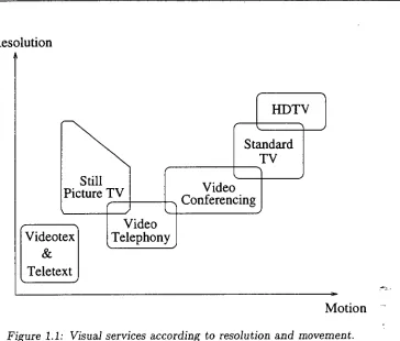
1.1 Visual services according to resolution and movement. 3

2.1 Block diagrams of a PCM encoder and decoder. 13

2.2 Block diagram of an encoder and decoder for Predictive Coding. . 15

2.3 Block diagram of Transform Coding technique. 18

2.4 Zig-zag scanning of transform coefficients 18

2.5 Example of DCT transform image compression. (a) Original image, (b) reconstructed image for a compression ratio of 8 : 1 and (c) reconstructed image for a compression ratio of 16 : 1. 22

2.6 Block diagram of pyramid coding 23

2.7 Example of pyramid coding. (a) Original image, (b) reduced image for k = 1, (c) reduced image for k = 2 and (d) reduced image for k = 3. . . 24

2.8 Block diagram of subband coding. 25

2.9 A simple single channel model of a transfer function for test stimuli. . 27

2.10 The contrast sensitivity function characteristic which has been explored by Kelly [55], Wilson and Giese [56], Wilson [57], King et al. [58] and

Bowon et al. [59] 28

(20)

List of Figures

2.11 The results of a simple experiment showing the relationship between visibility threshold and the distance from a dark-light transition. . . 29

2.12 Block diagram of psychovisual compression using the wavelet transform. 31

3.1 Typical basis functions and the time-frequency resolution of the wavelet transform, (a) basis functions and (b) the time-frequency plane. 37

3.2 The lattice of time-frequency location centers corresponding to lpj,„. . . 38

3.3 The orthogonal system of scaled and translated wavelets of the Haar basis. The upper plot shows 1/)( -1) of the dilated version and the lower

shows the translated versions of

7,b(x)

and

1/)(x

— 1) 39

3.4 The octave structure of V3 and 1473 42

3.5 Subband filtering scheme with exact reconstruction 43

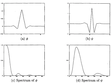
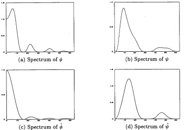
3.6 The scaling functions 20 and wavelets 20 and their spectra for the com-pactly supported wavelets with a maximum number of vanishing moments. 50

3.7 The scaling functions 24) and wavelets 20 and their spectra for the com-pactly supported wavelets with a maximum number of vanishing moments. 51

3.8 The scaling functions 4q and wavelets 40 and their spectra for the com-pactly supported wavelets with a maximum number of vanishing moments. 51

3.9 The scaling functions 60 and wavelets _01/) and their spectra for the com-pactly supported wavelets with a maximum number of vanishing moments. 52

3.10 The scaling functions 4 and wavelets 41/) and their spectra for near linear

phase wavelet bases. 55

3.11 The scaling functions 6q5 and wavelets 60 and their spectra for near linear

(21)

List of Figures

3.13 The coiflet and scaling functions for

L =

4 and their spectra. 59

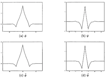
3.14 The B-spline scaling and wavelet functions for

L =

2 and

L =

2. (a) and

(b) for analysis, (c) and (d) for synthesis.

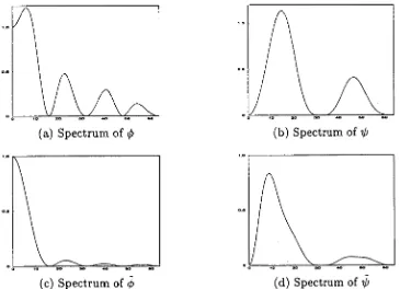
63 3.15 The spectra of the B-spline scaling and wavelet functions for

L =

2 and

L =

2. (a) and (b) for analysis, (c) and (d) for synthesis

63 3.16 The B-spline scaling and wavelet functions for

L =

2 and

L =

4. (a) and

(b) for analysis, (c) and (d) for synthesis.

64 3.17 The spectra of the B-spline scaling and wavelet functions for

L =

2 and

L =

4. (a) and (b) for analysis, (c) and (d) for synthesis

64 3.18 The B-spline scaling and wavelet functions with filters of similar length

for

L +

L =

8. (a) and (b) for analysis, (c) and (d) for synthesis. . . 66

3.19 The spectra of the B-spline scaling and wavelet functions with filters of

similar length for

L +

L =

8. (a) and (b) for analysis, (c) and (d) for

synthesis. 66

3.20 The biorthonormal close to orthonormal scaling and wavelet functions for

a = 0.03125. (a) and (b) for decomposition, (c) and (d) for reconstruction. 69

3.21 The spectra of the biorthonormal close to orthonormal scaling and wavelet

functions for a = 0.03125. (a) and (b) for decomposition, (c) and (d) for

reconstruction. 70

3.22 The biorthonormal close to orthonormal scaling and wavelet functions for

a = 0.05000. (a) and (b) for decomposition, (c) and (d) for reconstruction. 70

3.23 The spectra of biorthonormal close to orthonormal scaling and wavelet

functions for a = 0.05000. (a) and (b) for decomposition, (c) and (d) for

reconstruction.

71

(22)

x.xiv List of Figures

3.25 The spectra of biorthonormal close to orthonormal scaling and wavelet functions for a = 0.06250. (a) and (b) for decomposition, (c) and (d) for

reconstruction. 72

3.26 The biorthonormal close to orthonormal scaling and wavelet functions for a = 0.07500. (a) and (b) for decomposition, (c) and (d) for reconstruction. 72

3.27 The spectra of biorthonormal close to orthonormal scaling and wavelet functions for a = 0.07500. (a) and (b) for decomposition, (c) and (d) for

reconstruction. 73

4.1 Two-dimensional decomposition of an image for j = 1 using the pyramid

scheme. 78

4.2 Two-dimensional reconstruction of an image / -i_i for j = 1 using the

pyramid scheme. 79

4.3 Decomposition and reconstruction of an image for 3 levels of

decompo-sition (j — 3) 80

4.4 The spectrum of sensitivity function HVS. (a) Magnitude spectrum in 3D and (b) magnitude expressed as gray scale image 82

4.5 Impulse in subband W,F G at coordinate (47,47) in a 512 x 512 image

plane. 83

4.6 Example of the Daubechies wavelet with L = 2 and its spectrum, ex-pressed as a gray scale image. (a) the wavelet function, (b) the magnitude spectrum of the Fourier transform 84

4.7 The subband energy distributions of the wavelet coefficients obtained using the Daubechies wavelet for L = 2, where on the horizontal axis v corresponds to V4HH, a corresponds to WGH,1) corresponds to WHG, and

(23)

List of Figures XXV

4.8 The scanning order for the wavelet coefficients. 93

4.9 The block diagram of the statistical image compression scheme using the

wavelet transform 94

4.10 The block diagram of the psychovisual image compression scheme using

the wavelet transform 94

4.11 Performance of psychovisual image compression. (a) Original image "Lenna", (b) reconstructed image using the orthonormal Daubechies wavelet basis and (c) reconstructed image using the orthonormal near

linear phase wavelet basis 97

4.12 Performance of psychovisual image compression. (a) Reconstructed im-age "Lenna" using the orthonormal coiflet wavelet basis, (b) recon-structed image "Lenna" using the biorthonormal spline wavelet basis and (c) reconstructed image "Lenna" using the biorthonormal Laplacian

wavelet basis 98

4.13 Performance of psychovisual image compression, (a) The original and (b) the reconstructed test image "Airplane", (c) the original and (b) reconstructed test image "Bird" 102

4.14 Performance of psychovisual image compression. (a) The original and (b) the reconstructed test image "Peppers", (c) the original and (b)

reconstructed test image "Zelda" 103

4.15 The complete wavelet basis set for the decomposition of a signal 104

4.16 The complete wavelet basis set for the decomposition of an image. . . 104

4.17 Some permissible binary wavelet packets for 3 levels of decomposition. 105

(24)

xxvi List of Figures

4.19 The diagram for generating the wavelet function for the best basis ap-proach with 3 levels of decomposition. IWT is an inverse wavelet trans-form. HH, GH, HG and GG correspond to the wavelet functions of 1.1111 ,

AFGH , THG and TGG _{respectively. 109}

4.20 The selected bases for the decomposition of the test image "Lenna", (a) for the conventional approach and (b) for the best basis approach with three levels of decomposition. 113

4.21 The reconstruction test image "Lenna". (a) For the conventional

ap-proach and (b) for the best basis apap-proach. 113

5.1 The basic Block Matching Algorithm (BMA) 119

5.2 The block diagram of the simulation 122

5.3 Characteristic displacement vectors for the test image (a) "Miss Amer- ica", (b) "Salesman", (c) "Band", (d) "Skiing" and (e) "Scenic view". . 127

5.4 The "patch-work" characteristic of the variable block matching algorithm. 130

5.5 A possible subdivision of an original frame. 131

5.6 Examples of the subdivision of the test image sequence "Miss America" into a maximum block size of 8 x 8 and a minimum block size of 2 x 2 in the variable block size block matching algorithm. (a) The original image, (b) an example for a threshold value = 3, (c) an example for a threshold = 4, (d) an example for a threshold value = 5, (e) an example for a threshold value = 6 and (f) an example for a threshold value = 7. The brightest colour represents a block size of 8 x 8, the next brightest represents a block size of 4 x 4 and the darkest colour represents a block

(25)

List of Figures

xxvii

5.7 Examples of subdivision for the test image sequences "Salesman" and

"Band' into a maximum block size of 8 x 8 and a minimum block size

of 2 x 2 in the variable block size matching algorithm. (a) The original

image sequence "Salesman", (b) an example for a threshold value = 3, (c)

the original image sequence "Band" and (d) an example for a threshold

value = 3. The brightest colour represents a block size of 8 x 8, the next

brightest represents a block size of 4 x 4 and the darkest colour represents

a block size of 2 x 2

134 5.8 Examples of subdivision for the test image sequences "Skiing" and "Scenic

view" into a maximum block size of 8 x 8 and a minimum block size of

2 x 2 in the variable block size matching algorithm. (a) The original

im-age sequence "Skiing", (b) an example for a threshold value = 3, (c) the

original image sequence "Scenic view" and (d) an example for a

thresh-old value = 3. The brightest colour represents a block size of 8 x 8, the

next brightest represents a block size of 4 x 4 and the darkest colour

represents a block size of 2 x 2. 135

5.9 The block diagram of hybrid motion-compensated scheme. 142

5.10 A typical multiresolution motion estimation using a scaled block size.

M denotes a motion vector, the numbers 30, 31, 32 and 33 correspond

to the subbands HH, GH, HG and

GG

at the third decomposition

respectively. The numbers 21, 22 and 23 for the second decomposition

and 11, 12 and 13 for the first decomposition. A denotes the difference

in the position of the motion vector from the actual position. 144

5.11 The block diagram of the proposed scheme.

145 5.12 The comparison of the proposed scheme and standard DCT scheme for

image sequences "Miss America", (a) in terms of PSNR and (b) in terms

of total bits

150 5.13 The comparison of the proposed scheme and standard DCT scheme for

image sequences "Salesman", (a) in terms of PSNR and (b) in terms of

(26)

List of Figures

A.1 The standard single frame test image "Lenin" 159

A.2 The standard single frame test image "Airplane" 160

A.3 The standard single frame test image "Bird" 160

A.4 The standard single frame test image "Peppers" 160

A.5 The standard single frame test image "Zelda" 161

A.6 The first frame of the standard test image sequence "Miss America". . . 161

A.7 The first frame of the standard test image sequence "Salesman". . . . 161

A.8 The first frame of the standard test image sequence "Band" 162

A.9 The first frame of the standard test image sequence "Skiing" 162

A.10 The first frame of the standard test image sequence "Scenic view". . . 162

B.1 The viewing conditions. 164

B.2 The placement of the original and reconstructed images 165

C.1 The average energy distribution of twenty standard test images using orthonormal wavelet bases. (a) Daubechies wavelets and (b) near linear

phase wavelets. 167

C.2 The average energy distribution of twenty standard test images using orthonormal wavelet bases for coiflet wavelets. 168

C.3 The average energy distribution of twenty standard test images using biorthonormal wavelet bases. (a) Spline wavelets and (b) Laplacian

wavelets 168

(27)

List of Figures

xxix

D.2 The quantized coefficient distributions for the standard test images. (a) "Bird" image, (b) "Peppers" image and (c) "Zelda" image. 174

E.1 The block diagram for computing the WPSNR 178

G.1 The MAD value versus block number for the image sequence divided into subblocks of 2 x 2. (a) Test image "Miss America", (b) test image

"Salesman", (c) test image "Band", (d) test image "Skiing" and (e) test

image "Scenic view" 183

G.2 The MAD value versus block number for the image sequence divided into subblocks of 4 x 4. (a) Test image "Miss America", (b) test image "Salesman", (c) test image "Band", (d) test image "Skiing" and (e) test

(28)

List of Tables

1.1 Parameters of CCIR 601 Source Format Standard.

6 1.2 Parameters of the Common Intermediate Format

7 3.1 Filter coefficients

h(n)

for compactly supported Daubechies wavelet bases

for

L =

2,3, 4 and 6.

50 3.2 The regularity estimation of

LO

E

C. 3.3 Filter coefficients

h(n)

for near linear phase wavelet bases for

L =

4 and

L —

6

54 3.4 Filter coefficients

h(n)

for coiflets with

L =

2 and

L —

4

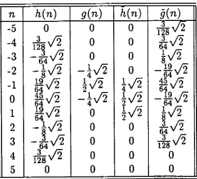
58 3.5 The B-spline filter coefficients

h(n), g (n), h(n)

and

:g(n)

for

L =

2 and

L =

2 .

62 3.6 The B-spline filter coefficients

h(n), g (n), h(n)

and §(n) for

L =

4 and

L -

2

62 3.7 The B-spline filter coefficients

h(n), g(n), h(n)

and

a(n)

for

L +

L =

8 with filters of similar length.

65 3.8 The Laplacian filter coefficients

h(n), g(m), h(n)

and

Tg(n)

for a = 0.03125. 68

3.9 The Laplacian filter coefficients

h(n), g(m), h(n)

and

§(n)

for a = 0.05000. 68

(29)

x3ocii

List of Tables

3.11 The Laplacian filter coefficients

h(n), g(n), h(n)

and

4(n)

for a = 0.07500. 69

4.1 Sensitivity factors of orthonormal Daubechies wavelet bases. 84

4.2 Sensitivity factors of orthonormal near linear phase wavelet bases. . 85

4.3 Sensitivity factors of orthonormal Coiflet wavelet bases. 85

4.4 Sensitivity factors of biorthonormal Spline wavelet bases. 86

4.5 Sensitivity factors of the biorthonormal close to the orthonormal wavelet

bases. 86

4.6 The optimum value of

K

for various wavelet bases 89

4.7 The optimum value of

q

for various wavelet bases. 92

4.8 Comparison of results between the Statistical and Psychovisual compres-sion schemes for constant bit rate of 0.40 bbp for the standard image

"Lenna" 95

4.9 Comparison of bit rates for Statistical and Psychovisual compression schemes for on the basis of comparable PSNR. 95

4.10 Effect on the coding performance by interchanging analysis and synthesis

wavelets 99

4.11 Results of the subjective assessment for statistical and psychovisual image compression using the standard image "Lerma" 100

4.12 Comparison of simulation results of three schemes 101

4.13 Performance of psychovisual image compression for the test images "Air-plane", "Bird", "Peppers" and "Zelda" 101

4.14 Sensitivity factors for the first decomposition 110

(30)

List of Tables xxxiii

4.16 Sensitivity factors for the third decomposition

111 4.17 Comparison of the WPSNR for the

.

conventional and best basis approaches. 113

5.1 Performance of the fixed block size BMA-MC for the image sequence

"Miss America"

124 5.2 Performance of the fixed block size BMA-MC for the image sequence

"Salesman"

124 5.3 Performance of the fixed block size BMA-MC for the image sequence

"Band"

125 5.4 Performance of the fixed block size BMA-MC for the image sequence

"Skiing"

125 5.5 Performance of the fixed block size BMA-MC for the image sequence

"Scenic view"

126 5.6 Results for the variable block size BMA-MC for the image sequence "Miss

America"

136 5.7 Results for the variable block size BMA-MC for the image sequence

"Salesman"

137 5.8 Results for the variable block size BMA-MC for the image sequence

"Band"

138 5.9 Results for the variable block size BMA-MC for the image sequence

"Skiing"

139 5.10 Results for the variable block size BMA-MC for the image sequence

"Scenic view"

140 5.11 Performance of the existing scheme using the DCT transform as shown

(31)

xxxiv List of Tables

5.12 Performance of the existing scheme using the wavelet transform. This scheme is similar to that proposed by Zhang [133] except that a constant step size in the quantization is used so as to allow a comparison with our method that incorporates the HVS 146

5.13 Performance of our proposed scheme for the image sequence "Miss Amer-

ica" 146

5.14 Performance of our proposed scheme for the image sequence "Salesman". 147

5.15 Performance of our proposed scheme for the image sequence "Band". . . 148

5.16 Performance of our proposed scheme for the image sequence "Skiing". . 148

5.17 Performance of our proposed scheme for the image sequence "Scenic view".149

C.1 The average energy in the subbands for the orthonormal Daubechies

wavelet bases 169

C.2 The average energy in the subbands for the orthonormal near linear

C.3 The average energy in the subbands for the orthonormal Coiflet wavelet

bases. 170

C.4 The average energy in the subbands for the biorthonormal Spline wavelet

bases. 170

C.5 The average energy in the subbands for the biorthonormal close to

or-thonormal wavelet bases (Laplacian wavelet bases) 171

D.1 The Huffman code words for the transform coefficients. 175

D.2 The Huffman code words for the run length. 176

(32)

List of Tables

G.1 The MAD values for the test image sequence "Miss America" 181

G.2 The MAD values for the test image sequence "Salesman" 182

G.3 The MAD values for the test image sequence "Band" 182

G.4 The MAD values for the test image sequence "Skiing" 182

(33)

Chapter 1 Introduction

Nowadays, video applications such as digital laser disc, electronic camera, videophone and video conferencing systems, image and interactive video tools on personal comput-ers and workstations, program delivery using cable and satellite, and high-definition television (HDTV) are available for visual communications. Many of these applica-tions, however, require the use of data compression because visual signals require a large communication bandwidth for transmission and large amounts of computer mem-ory for storage. In order to make the handling of visual signals cost effective it is important that their data be compressed as much as possible. Fortunately, visual sig-nals contain a large amount of statistically and psychovisually redundant information. By removing this unnecessary information, the amount of data necessary to adequately represent an image can be reduced.

The removal of unnecessary information generally can be achieved by using either statis-tical compression techniques or psychovisual compression techniques. Both techniques result in a loss of information, but in the former the loss may be recovered by signal processing such as filtering and inter or intra-polation. In the latter, information is in fact discarded, but in way that is not perceptible to a human observer. The lat-ter technique offers much grealat-ter levels of compression but it is no longer possible to perfectly reconstruct the original image. While the aim in psychovisual coding is to keep these differences at an imperceptible level, psychovisual compression inevitably involves a tradeoff between the quality of the reconstructed image and the compression

(34)

2

Chapter 1. Introduction

rate achieved. This tradeoff can often be assessed using mathematical criteria, although a better assessment is in general provided by a human observer.

The compression techniques can be applied to single or still images and to sequences of video images. There are two main techniques of image compression. The first technique, known as intra-frame aiding, relies on removing the spatial redundancies in the images a single frame at a time. Very often these techniques are simply called image compression techniques. The second technique, inter-frame coding, exploits the redundancies caused by temporal correlations as well as spatial correlations in successive video images. This technique holds the promise of a significantly large reduction in the data required to transmit the image sequence.

There are numerous ways to achieve compression in both image compression and video compression techniques. Predictive coding and transform coding are widely used for image compression techniques. Predictive schemes compress each of the picture ele-ments (pixels) by quantizing the difference between a predicted value whose value is based on the previous pixels. Transform coding especially using the Discrete Cosine Transform (DCT) is an international standard and one of the most powerful compres-sion techniques [6]. In successive video images, each picture frame is typically very close to those temporally adjacent to it and each picture usually contains a background and a number objects, which are essentially unchanging from frame to frame. When some of the objects are moving, and assuming that movement in the picture is only a shift or displacement of object position, then the location of a pixel or a group of pixels on the same part of the moving object can be predicted from the previous frame. This technique is called motion compensation.

This thesis is largely concerned with psychovisual compression techniques. The appli-cations of intra-frame and inter-frame coding in conjunction with transform coding and psychovisual compression are presented in this study.

1.1 Visual Communication

(35)

Video

, Conferencing

HDTV

Standard

TV

Still

Picture

TV

Videotex

Teletext

Video

Telephony

1.1. Visual Communication

3

Resolution

A

[image:35.559.138.502.87.397.2]

Motion

Figure 1.1: Visual services according to resolution and movement.

visual communication services. These visual communication services can be distin-guished as "interactive services" and "distribution services" [7]. Interactive services contain conversation services, messaging services and retrieval services. Conversation services provide dialogue communication with real time end-to-end information transfer such as data processing. Messaging services offer user-to-user communication between individual users via storage units with store-and-forward functions. Retrieval services can retrieve information stored in information centres and, in general, be provided for public use. The distribution services, also known as broadcast and narrowcast services, provide the customer with an information flow from a central source. Figure 1.1 illus-trates a collection of some of the common video and image-based services in accordance to resolution and movement.

Videotex, Teletext and Still Picture TV

(36)

4

Chapter 1. Introduction

retrieved from the computer on a modified television set or specially designed visual display unit. Videotex services enable information in the forms of words, pictures and graphics to be transmitted and displayed electronically on demand, and with which the user can interact by sending electronic messages or commands in response.

Teletext [9] refers to any broadcasting system which displays selected frames of infor-mation as they are being continuously recycled by the originator of the signal. The broadcast signal is generated with the aid of a computer. The information is prepared and stored digitally and is usually broadcast as a portion of the regular television sig-nal. Still picture TV [7, pp. 8-111, often referred to as slow-scan television or freeze frame, was developed for applications where the update of movement is not critical.

Video Conferencing

Video conferencing systems are used for two or more groups of people at widely sepa-rated locations who wish to communicate in real time, both visually and orally [10] [11]. The objective of video conferencing is to save time and costs that would be incurred by physically bringing all of the conference participants to the same location and to be a useful alternative form of communication between co-workers, business associates and managerial staff. During the video conference several types of information can be transmitted such as sound, still and moving video, messages, handwriting and facsimile.

(37)

1.2. Source Format of Video Signals 5

Video Telephony

Video telephony is a bidirectional service in which speech and moving images are com-municated as in normal face-to-face conversation, including facial expressions, posture and gestures [11, pp. 115-120) [13]. The picture information transmitted is sufficient for the adequate representation of smooth motions of persons displayed in head and shoulder view. The video telephone has a mode for normal telephone, and narrow band video telephony can basically be seen as scaled-down video conferencing with limited functionality. The standard transmission format of Quadrature CIF (QCIF) and tem-poral frequencies below 15 frames-per-second with grey-scale images are commonly used for video telephony.

Multimedia Communication

Recent advances in networking, storage, personal computers, workstations and inte-grated circuit technology as well as demands for better communication accommodations have fostered tremendous interest in the development of multimedia communication sys-tems [14]. Multimedia communication [15) is the field referring to the representation, storage, retrieval and dissemination of machine-processable information expressed in multimedia, such as text, audio, voice, graphics, image and video in a range of config-urations to suit the end user.

Applications in education and training, office and business systems, information and point of sales are the main multimedia services [16]. In all of these different fields, the visual aspects of the multimedia applications are still image, motion video and graphics based.

1.2 Source Format of Video Signals

(38)

PAL

NTSC

Parameters

625/50

525/60

sampling frequency

sampling structure

number of active lines

number of pixels

per active line

luminance (Y)

chrominance (U)

chrominance (V)

Field frequency

quantization

13.5 MHz (luminance Y)

6.75 MHz (chrominance U,V)

orthogonal

576 720 pixels/line

360 pixels/line

50 Hz

8 bit PCM

13.5 MHz

6.75 MHz

orthogonal

480 720 pixels/line

360 pixels/line

59.94 Hz

8 bit PCM

6

Chapter 1. Introduction

NTSC systems. The PAL system is used in Europe (with the exception of France which

uses SECAM) and Australia with the main scanning standard of 50 fields-per-second

and 625 lines-per-frame. The NTSC system is used in North America and Japan with

60 fields-per-second and 525 lines-per-frame. These standards have been adopted by

the CCIR recommendation 601 [17]and are depicted in Table 1.1.

Table 1.1: Parameters of CCIR 601 Source Format Standard.

The luminance component Y is sampled at 13.5 MHz and the chrominance components

U and V at 6.75 MHz. Therefore the number of chrominance pixels is half the number of

luminance pixels. The number of bits in one frame for either standard can be computed

by

Tb = Hor(m) x V er(n) x bPP

where

Tb

denotes the number of bits in one frame,

bpp

the number of bits per pixel,

H or (m)

the number of horizontal samples and Ver(n) the number of active lines. When

dealing with PAL and NTSC systems, the total number of bits becomes

Tb _{PAL =}

(720 x 576 x 8) + 2(360 x 576 x 8)

= 6, 635, 520bits/frame,

and

Tb NTSC = (720

x 480 x 8) + 2(360 x 480 x 8)

= 5, 529, 600bits/frame,

(39)

1.2. Source Format of Video Signals

7

The overall bit rate is defined by

Ct = Tb X

F

r

where

F

r

denotes the frame rates. The frame rate,

F

r

,

for PAL is 25 Hz and for NTSC

is approximately 30 Hz. Therefore the channel capacity to transport CCIR rec. 601

signals is

C

t

PAL =

166 Mbps and Ct

NTSC =

166 Mbps respectively.

Common Intermediate Format

Many regions have different national television standards and it is therefore necessary

to convert standards for use in inter-regional television broadcasting. The Common

Intermediate Format (CIF) was created when an agreement was reached to overcome

the differences between inter-regional television standards [7, pp. 31-33]. The NTSC

system actually has 480 active lines, whereas the PAL system has 576 active lines. It

was agreed internationally that the countries using NTSC would convert the number of

lines towards 288 non-interlaced lines and the countries using PAL would convert the

number of fields. The basic parameters for CIF are depicted in Table 1.2. A fallback

mode is based on one quarter of the CIF, and is denoted by QCIF.

CIF QCIF

Number of active lines

Luminance (Y)

288

144 Chrominance (U, V)

144

72 Number of active pixels per line

Luminance (Y)

360

180 Chrominance (U, V)

180

90

(40)

8

Chapter 1. Introduction

1.3 Structure of the thesis

The main focus of this thesis is the design of psychovisual image and video compres-sion schemes using the wavelet transform. The next two chapters describe the available techniques for image and video coding and the chapter after that introduces the wavelet transform. The last two chapters focus on the design of a psychovisual image compres-sion and video comprescompres-sion technique using the wavelet transform respectively.

Chapter II describes an overview of the techniques available for image and video com-pression of visual information. The statistical image comcom-pression techniques such as PCM, Predictive coding, Transform coding, Pyramid coding and Sub-band coding, as well as psychovisual image coding techniques are presented. Combinations of these techniques are also outlined.

Chapter III describes the wavelet transform which is a useful sub-band coding scheme based on a multiresolution decomposition of signals and images. The wavelet basis functions can be generated using many different functions. We construct, in particular, wavelet bases by using the methodology for generating compactly supported orthonor-mal and biorthonororthonor-mal wavelet bases. The properties of such wavelets are also pre-sented. These wavelet bases are then employed for statistical as well as psychovisual image compression.

Chapter IV explores psychovisual image compression techniques using the wavelet transform coefficients. The application of the wavelet transform in signal and image processing can be divided into two schemes: the conventional approach based directly on Mallat's multiresolution wavelet decomposition [18] and the best basis approach [19]. This chapter firstly examines the conventional scheme using both psychovisual com-pression as well

as

statistical compression with various wavelet bases. The simulation results of both the statistical and psychovisual schemes are compared for the various wavelet bases. Only the wavelet bases which produced the best result are applied to the best basis approach and used for a comparison with the conventional scheme.

(41)

1.3. Structure of the thesis 9

is examined, in particular for the conventional wavelet transform scheme. The best basis scheme is not carried out using the multiresolution motion compensation scheme, due to a large computational cost that renders the algorithm impractical for real-time applications.

(42)

(43)

Chapter 2 From Image to Video

Compression

2.1 Introduction

An image is usually represented by a two-dimensional array of numbers over a rectan-gular or square lattice. The gray level variations are used to represent the information in the image. In many practical cases, an image is often defined over a 256 x 256 or 512 x 512 lattice. Typically each pixel is represented by 8 bits, corresponding to a gray level variation between 0 and 255. Storing a 512 x 512 image requires approximately 2096 Kbits memory which constitutes a significant quantity of memory. It is therefore desirable to compress the information in the image into a considerably fewer number of bits whilst maintaining the ability to reconstruct the image such that it is close to the original image. Thus an image needs to be compressed for efficient data storage applications or to reduce the bandwidth capacity required to transmit the image.

The applications of image data compression, in general, are primarily in the trans-mission and storage of information. In transtrans-mission, applications such as broadcast television, teleconferencing, videophone, computer-communication, remote sensing via satellite or aircraft, etc., require the compression techniques to be constrained by the need for the real time compression and on-line consideration which tends to severely

(44)

12

Chapter 2. From Image to Video Compression

limit the size and hardware complexity. In storage applications such as medical images, educational and business documents, etc., the requirements are less stringent because much of the compression processing can be done off-line. However, the decompression or retrieval should still be quick and efficient to minimise the response time [20].

When dealing with images the data compression techniques may be divided into two schemes. There are image compression techniques and video compression techniques. The former techniques exploit the redundancy in the images a single frame at a time, whilst the latter ones exploit the temporal correlations between successive images in the sequence. If the sequence is highly correlated, this technique holds the promise of significantly greater compression in the data when transmitting an image sequence. If there exists no correlation within the various images making up the sequence, the problem of video compression reduces to one of image compression, with each individual image within the sequence treated separately [21].

All images of interest usually contain a considerable amount of statistically and subjec-tively superfluous information [11, pp. 148-150]. A statistical image compression tech-nique exploits statistical redundancies in the information in the image. This techtech-nique reduces the amount of data to be transmitted or to be stored in an image without any information being lost. The alternative is to discard the subjective redundancies in an image, which leads to psychovisual image compression. These psychovisual techniques rely on properties of the Human Visual characteristic System (HVS) to determine which features will not be noticed by a human observer.

In the following section a brief overview of image coding and video coding in terms of compression techniques is provided. Both statistical and psychovisual compression schemes are presented. More general reviews on the subjects can be found in [7] [11]

[20] [22] [23] [24] [25].

2.2 Statistical Image Compression Techniques

(45)

2.2. Statistical Image Compression Techniques

13

discarded and therefore a perfect or near perfect representation of the image can be reconstructed. In this section we discuss some compression methods which belong to the class of statistical Compression techniques.

2.2.1 Pulse Code Modulation (PCM)

PCM, also known as analog to digital conversion, is a simple method to represent the discrete amplitudes of signal information into binary code words. It has not been used for television up until 1951, although it was developed in the late 1930's. Since then it has been used as a video digitizing scheme for the purposes of storage and transmission.

The block diagrams of a PCM encoder and decoder are shown in Figure 2.1. The input signal, a one-dimensional raster scanned waveform of the image is firstly band-limited by an anti-aliasing filter and then sampled at the Nyquist sampling rate, where the Nyquist sampling rate is twice the highest frequency in the input signal. The resulting sampled signal is then quantized to 2 N discrete amplitude levels. Each level

is represented by a binary code word containing N bits. This scheme is also known as fixed word-length coding. At the decoder, these binary code words are converted to a sequence of discrete amplitude levels which are then lowpass filtered to obtain a reconstruction of the original signal. The number of bits needed to code a pixel using PCM depends on the type of image. In general, 128 or 256 levels (7 or 8 bits) are sufficient for a monochrome image [11, pp. 304-3071.

Input Signal

PCM code Band limited

Filter Sampler Quantizer

Binary code-word

(a) Encoder PCM

PCM code

code-word-amplitude Converter

Lowpass Filter

reconstructed Signal

(b) Decoder PCM

(46)

14

Chapter 2. From Image to Video Compression

In order to obtain a perfectly reconstructed image from the coded data, the number of quantizing levels, 2 N , must be sufficient to ensure that the decoded image is not significantly different from the original image. Thus, in this simple scheme each pixel is represented by N bits.

2.2.2 Predictive Coding

In PCM coding, the successive inputs to the quantizer are treated independently, and thus there is no exploitation of any redundancy present in images. Visual images contain statistical redundancies such as the correlation between adjacent pixels that are spatially close to each other [11, pp. 313-3211. Predictive coding techniques exploit this correlation. The principle of this technique is to predict or to approximate the next sample in order to remove the mutual redundancy between successive samples and quantize only the difference or new information.

The block diagram of a predictive coder and decoder is shown in Figure 2.2. The predictive coder has three basic components; namely, a Predictor, Quantizer and Code Assigner. The basic principle of this technique is to predict the value of the current pixel based on the previously coded pixel that has been transmitted [26]. The prediction error or differential signal is quantized into a set of

N

discrete amplitude levels, coded using either a fixed or variable word-length code and then transmitted. The quantizer depends on the number of levels of quantization. If the quantizer has only 2 levels, the predictive coding is known as Delta Modulation (DM) [27]. When the quantizer has more than 2 levels the predictive coding is known as Differential Pulse Code Modulation (DPCM). Since, DM uses only 2 quantization levels, the sampling rate has to be several times the Nyquist rate in order to avoid slope overload and get an adequate picture quality [11, pp. 313-321].

The predictor for DPCM can be either linear or non-linear, depending on whether the prediction is a linear or non-linear combination of previously transmitted values. Linear prediction has been extensively studied [28] [29] and has the general form

I

n =

E

apIn-p (2.1)

p=1

(47)

uantizer

Code

To

Predictor

Input

Assigner

_Channel

2.2. Statistical Image Compression Techniques

15

(a) Coder

From

Channel

Decoder

Output

Predictor

(b) Decoder

Figure 2.2: Block diagram of an encoder and decoder for Predictive Coding.

and

P

is the order of prediction. The prediction coefficients {ap } can be obtained by minimising the mean square prediction error (MSPE),

E(I

n

—

fn)2. By using the optimum coefficients, the mean square prediction error is given by [11, pp. 313-321]

optimufn(MSPE) = o-2 —

E

apdp (2.2) p=1

(48)

16 Chapter 2. From Image to Video Compression

2.2.3 Code word assignment and Huffman Coding

In both PCM and DPCM schemes, the output quantized levels are coded by the assign-ment of code words before being stored or transmitted. In general, the PCM scheme uses constant or fixed length N bit binary words to represent the various signal levels. In practice, however, the probability distribution of the output quantizer levels, espe-cially for DPCM, is highly nonuniform. This naturally lends itself to a representation using code words of variable length [11, pp. 379-380] [30]. The average number of bits per word can be reduced if the output quantized levels having a high probability are assigned short code-words, while the output quantized levels having a lower probability are assigned longer code words. This method is called variable word-length coding or entropy coding [11, pp. 148-150]. Let the output quantized level be denoted by b with probability of occurence P(b). It is assigned a code word of length WL(b) bits. Then the average code word length WL can be calculated by

wL,

= E

wL(b)P(b) [bits/pixel]. (2.3)

The average code word length WL cannot be made arbitrarily small, however, and still must be correctly decoded by a receiver [11, pp. 148-1501. The average code word length WL should satisfy the lower bound which is derived from information theory [31], and is given by

He(B) < W L (2.4)

where He(B) is the entropy,

He(B) = —

E

P(b)log2P(b) [bits/pixel]. (2.5)

(49)

2.2. Statistical Image Compression Techniques

17

2.2.4 Transform Coding

The previous coding techniques attempt to reduce the correlation that exists among adjacent image pixel intensities. Transform coding [11] [39] [40] attempts to represent an image by uncorrelated data, using a reversible linear transformation. In the most general form, an image is sampled and subdivided into small square blocks of

N

x

N

pixels. The transformation of one of these subblocks into another domain, usually frequency-related, is denoted by

N-1 N-1

AU,

V) =

E E

n) f ,,ker(u7v;m,n), for u, v; m, n = 0, 1, ,

N —

1 (2.6) m=0 n=0

where

f

ker,U, V; m( , n) is the forward transform kernel. The original image subblocks

can then be recovered by

N-1 N-1

n) =

E E o

ker

(u,v;

m,

n), for u, v; m, n = 0, 1, ,

N —1

u=0 v=0

(2.7)

where i( ker,U, V; m, n) is an inverse transform kernel.

The objective of transform coding is to represent the energy of the original subblock by a small fraction of the transform coefficients, a process called energy compaction. This means that only the transform coefficients that adequately represent the image need to be transmitted.

The block diagram of the transform coding technique is shown in Figure 2.3. The original image is subdivided into small square subblocks and transformed. The non-zero transformed subblock coefficients in which all the energy is contained are quantized and encoded before transmission. DPCM is, in general, used for the coding scheme. At the receiver, the code words are decoded and then dequantized. These received subblocks are then inverse transformed to obtain the reconstructed image.

(50)

18

Chapter 2. From Image to Video Compression

Original Image

Subdivide

Image 1■111.1 Transform

Subblocics Quantizer

Code Words

To

Channel

(a) Transmitter

From

Channel Decoder Dequantizer

Inverse Transform

Image

Rebuilder Reconstructed Image

(b) Receiver

Figure 2.3: Block diagram of Transform Coding technique.

tables are simply Huffman coded. In order to minimise the amount of information required to represent a subblock, the quantized coefficients need to be scanned before coding. There are many ways in which an image can be scanned but the zig-zag scanning method illustrated by Figure 2.4 is the most commonly used and has been accepted as part of an international coding scheme standard [35] [36] [37].

•

• • •

•

• • • • • • • • •

• • • • • •

• • •

•

• • • • • • •

• • • • • • • • •

• • •

• • • • •

•

• • •

•

• • • • • • •

•

• Figure 2.4: Zig-zag scanning of transform coefficients.

(51)

2.2. Statistical Image Compression Techniques

19

lation statistics of the original subblocks [11, pp. 392-400], which makes it difficult to implement. Consequently, the KLT is not often used in practice, but rather provides an optimal linear transformation for bench-mark comparison of other techniques. There are many different less optimal linear transforms which produce compactly efficient al-gorithms and which are independent of the statistics of the input images [11]. Some of the more important transforms are the discrete Fourier transform (DFT) [34], Walsh-Hadamard transform (WLH) [38] and discrete Cosine transform (DCT) [39]. Recently, the wavelet transform (WT) has also be used in transform image coding.

Discrete Fourier Transform

The DFT is a very common separable unitary and symmetric linear transform, which transforms the spatial domain into the frequency domain. The basis kernels of the DFT are the complex exponentials. The forward and inverse DFT kernels are given by

fker (U, V; M, 71) =

k

e

-i2L

A

rr(um+vn)

iker(U, V; in, n) =* e±iji(um2 -1-vn)

(2.8)

where i = ILI A major feature of the DFT is the existence of a fast algorithm for its computation called the Fast Fourier transform (FFT). When

N

is a power of 2, the DFT requires approximately N2 complex operations, whilst the FFT requires only Nlog2 N [11, pp. 380-388].

Walsh-Hadamard Transform

The WI-IT [38] is also a separable unitary and symmetric transform, which has the same forward and inverse kernels. The basis kernel of the WHT is denoted by

fker(U) vi m, n) = iker(U11); m, n) = TIT (-1)P(m'n'u'v) (2.9)

with

log2 N-1

p(m,

n; x, y) =

E (u

k

m, +

vk nk) (2.10) k=0

Psychovisual video coding using wavelet transform