Simulation based optimization of agent scheduling in multiskill call centers

SIMULATION-BASED OPTIMIZATION OF AGENT SCHEDULING IN MULTISKILL CALL CENTERS

Athanassios N. Avramidis, Michel Gendreau, Pierre L’Ecuyer

D´epartement d’Informatique et de Recherche Op´erationnelle Universit´e de Montr´eal, C.P. 6128, Succ. Centre-Ville

Montr´eal (Qu´ebec), H3C 3J7, CANADA

Ornella Pisacane

Dipartimento di Elettronica Informatica e Sistemistica

Universit`a della Calabria, Via P. Bucci, 41C, Arcavacata di Rende (CS), ITALY

May 15, 2007

ABSTRACT

We examine and compare simulation-based algorithms for solving the agent scheduling problem in a multiskill call center. This problem consists in minimizing the total costs of agents under constraints on the expected service level per call type, per period, and aggregated. We propose a solution approach that combines simulation with integer or linear programming, with cut generation. In our numerical experiments with realistic problem instances, this approach performs better than all other methods proposed previously for this problem. We also show that the two-step approach, which is the standard method for solving this problem, sometimes yield solutions that are highly suboptimal and inferior to those obtained by our proposed method.

INTRODUCTION

The telephone call center industry employs millions of people around the world and is fast growing. A few percent saving in workforce salaries easily means several million dollars. Call centers often handle several types of calls distinguished by the required skills for delivering service. Training all agents to handle all call types is not cost-effective. Each agent has a selected number of skills and the agents are distinguished by the set of call types they can handle (also called their skill set). When such skill constraints exist, we speak of a multiskill call center. Skill-based routing(SBR), or simplyrouting, refers to the rules that control the call-to-agent and agent-to-call assignments. Most modern call centers perform skill-based routing (Koole and Mandelbaum 2002, Gans et al. 2003). In a typical call center, inbound calls arrive at random according to some complicated stochastic processes, call durations are also random, waiting calls may abandon after a random patience time, some agents may fail to show up

to work for any reason, and so on. Based on forecasts of call volumes, call center managers must decide (among other things) how many agents of each type (i.e., skill set) to have in the center at each time of the day, must construct working schedules for the available agents, and must decide on the call routing rules. These decisions are made under a high level of uncertainty. The goal is typically to provide the required quality of service at minimal cost. The most common measure of quality of service is the service level(SL), defined as the long-term fraction of calls whose time in queue is no larger than a given threshold. Frequently, multiple measures of SL are of interest: for a given time period of the day, for a given call type, for a given combination of call type and period, aggregated over the whole day and all call types, and so on. For certain call centers that provide public services, SL constraints are imposed by external authorities, and violations may result in stiff penalties (CRTC 2000).

to estimate the SL; it can be estimated accurately only by long (stochastic) simulations. Scheduling problems in general are difficult (they are NP-hard) even in deterministic settings where each solution can be evaluated quickly and exactly. When this evaluation requires costly and noisy simulations, as is the case here, solving the problem exactly is even more difficult and we must settle with methods that are partly heuristic.

Staffing in the single-skill case (i.e., single call type and single agent type) has received much attention in the call center literature. Typically, the workload varies considerably during the day (Gans et al. 2003, Avramidis et al. 2004, Brown et al. 2005), and the planned staffing can change only at a few discrete points in time (e.g., at the half hours). It is common to divide the day into several periods during which the staffing is held constant and the arrival rate does not vary much. If the system can be assumed to reach steady-state quickly (relative to the length of the periods), then steady-state queueing models are likely to provide a reasonably good staffing recommendation for each period. For instance, in the presence of abandonments, one can use an Erlang-A formula to determine the minimal number of agents for the required SL in each period (Gans et al. 2003). When that number is large, it is often approximated by the square root safety staffing formula, based on the Halfin-Whitt heavy-traffic regime, and which says roughly that the capacity of the system should be equal to the workload plus some safety staffing which is proportional to the square root of the workload (Halfin and Whitt 1981, Gans et al. 2003). Scheduling problems are often solved in two separate steps (Mehrotra 1997): After an appropriate staffing has been determined for each period in the first step, a minimum-cost set of shifts that covers this staffing requirement can be computed in the second step by solving a linear integer program. However, the constraints on admissible working shifts often force the second step solution to overstaff in some of the periods. This drawback of the two-step ap-proach has been pointed out by several authors, who also proposed alternatives (Keith 1979, Thompson 1997, Hen-derson and Mason 1998, Ingolfsson et al. 2003, Atlason et al. 2004). For example, the SL constraint is often only for the time-aggregated (average) SL over the entire day; in that case, one may often obtain a lower-cost scheduling solution by reducing the minimal staffing in one period and increasing it in another period. Atlason et al. (2004) devel-oped a simulation-basedmethodology to optimize agent’s scheduling in the presence of uncertainty and general SL constraints, based on simulation and cutting-plane ideas. Linear inequalities (cuts) are added to an integer program until its optimal solution satisfies the required SL constraints. The SL and the cuts are estimated by simulation.

In themultiskill case, the staffing and scheduling problems are more challenging, because the workload can be covered by several possible combinations of skill sets, and the

routing rules also have a strong impact on the performance. Staffing a single period in steady-state is already difficult; the Erlang formulas and their approximations (for the SL) no longer apply. Simulation seems to be the only reliable tool to estimate the SL. Cez¸ik and L’Ecuyer (2007) adapt the simulation-basedmethodology of Atlason et al. (2004) to the optimal staffingof a multiskill call center for asingle period. They point out difficulties that arise with this methodology and develop heuristics to handle them. Avramidis et al. (2006) solve the same problem by using neighborhood search methods combined with an analytical approximation of SLs, with local improvement via simulation at the end. Pot et al. (2007) impose a constraint only on the aggregate SL (across all call types); they solve Lagrangean relaxations using search methods and analytical approximations. Some authors have developed queueing approximations for the case of two call types, via Markov chains and under simplifying assumptions; see Stolletz and Helber (2004) for example. But here we are thinking of 20 to 50 call types or more, which is common in modern call centers, and for which computation via these types of Markov chain models is clearly impractical.

For themultiskill scheduling problem, Bhulai et al. (2007) propose a two-step approach in which the first step deter-mines a staffing of each agent type for each period, and the second step computes a schedule by solving an IP in which this staffing is the right-hand side in key constraints. A key feature of the IP model is that the staff-coverage constraints allowdowngradingan agent into any alternative agent type with smaller skill set, separately for each period. Bhulai et al. (2007) recognize that their two-step approach is generally suboptimal.

In this paper, we propose asimulation-basedalgorithm for solving the multiskill scheduling problem, and compare it to the approach of Bhulai et al. (2007). This algorithm extends the method of Cez¸ik and L’Ecuyer (2007),which solves a single-period staffing problem. In contrast with the two-step approach, our method optimizes the staffing and the scheduling simultaneously. Our numerical experiments show that our algorithm provides approximate solutions to large-scale realistic problem instances in reasonable time(a few hours). These solutions are typically better, sometimes by a large margin (depending on the problem), than the best solutions from the two-step approach. We are aware of no competitive faster method.

MODEL FORMULATION

problem formulations here do not depend on the details of this model.

There are K call types, labeled from 1 to K, and I agent types, labeled from 1 toI. Agent typeihas the skill setSi⊆ {1, . . . ,K}. The day is divided inPperiod, labeled from 1 to P. Thestaffing vectorisy= (y1,1, . . . ,y1,P, . . . ,yI,1, . . . ,yI,P)t where yi,p is the number of agents of type i available in period p. Given y, the service level (SL) in period p is defined as

gk,p(y) =E[Sg,k,p]/E[Sk,p+Ak,p],

whereSk,pis the number of type-kcalls that arrive in period p,Sg,k,p is the number of those calls that get served after waiting at mostτk,p(a constant called theacceptable waiting time), and A_k,p is the number of those calls that abandon in period pafter waiting at least τk,p. Aggregate SLs, per call type, per period, and globally, are defined analogously. Given acceptable waiting timesτp,τk, andτ, the aggregate

SLs are denoted bygp(y),gk(y)andg(y)for periodp, call typek, and overall, respectively.

Ashiftis defined by specifying the time periods in which an agent is available to handle calls. Let{1, . . . ,Q} be the set of all admissible shifts. We assume that this set is the same for all agent types. The admissible shifts are specified via aP×Q matrix A₀ whose element (p,q)is ap,q=1 if an agent with shiftq works in period p, and 0 otherwise. A vectorx= (x1,1, . . . ,x1,Q, . . . ,xI,1, . . . ,xI,Q)t, wherexi,qis the number of agents of typeiworking shiftq, is aschedule. The cost vector is c= (c1,1, . . . ,c1,Q, . . . ,cI,1, . . . ,cI,Q)t, where ci,q is the cost of an agent of type iwith shift q. To any given shift vector x, there corresponds the staffing vector y=Ax, whereAis a block-diagonal matrix withIidentical blocks A0, if we assume that each agent of type i works as a type-i agent for her entire shift.

However, following Bhulai et al. (2007), we also allow an agent of typelto be downgraded to an agent with smaller skill set, i.e., of typeipwhereSip⊂Sl, in any time periodpof her

shift. DefineS_i+={j:Sj⊃Si},Si−={j:Sj⊂Si}, and letzl,i,pbe the number of type-lagents that are downgraded to typeiduring periodp. These are theskill transfervariables. A schedule x= (x1,1, . . . ,x1,Q, . . . ,xI,1, . . . ,xI,Q)t is said to cover the staffingy= (y1,1, . . . ,y1,P, . . . ,yI,1, . . . ,yI,P)tif for i=1, . . . ,Iandp=1, . . . ,P, there are nonnegative integers zl,i,p for l∈Si+ andzi,l,pfor l∈Si−, such that

Q

∑

q=1

ap,qxi,q+

∑

i

zl,i,p−

∑

i

zi,l,p ≥ yi,p. (1)

These inequalities can be written in matrix form as Ax+ Bz≥y, wherezis a column vector whose elements are the zl,i,p variables andB is a matrix whose entries are in the

set{−1,0,1}. With this notation, the scheduling problem can be formulated as

(P0) : [Scheduling problem] min ctx=∑Ii=1∑Qq=1ci,qxi,q

s.t.

Ax+Bz≥y

gk,p(y)≥lk,p for 1≤k≤K and 1≤p≤P gp(y)≥lp for 1≤p≤P

gk(y)≥lk for 1≤k≤K g(y)≥l

x≥0, z≥0, y≥0 and integer

wherelk,p,lp,lk andl are given constants.

In practice, a given agent often works more efficiently (faster) when handling a smaller number of calls (i.e., if his skill set is artificially reduced). The possibility of down-grading agents to a smaller skill set for some periods can sometimes be exploited to take advantage of this increased efficiency. In case where the agent’s speed for a given call type (in the model) does not depend on its skill set, one might think intuitively that downgrading cannot help, because it only limits the flexibility of the routing. This would be true if we had an optimal dynamic routing of calls. But in practice, an optimal dynamic routing is too complicated to compute and simpler routing rules are used instead. These simple rules are often static. Then, down-grading may sometimes help by effectively changing the routing rules. Clearly, the presence of skill transfer vari-ables in (P0) cannot increase the optimal cost, it can only reduce it.

Suppose we consider a single period, say period p, and we replace gk,p(y) andgp(y) by approximations that depend on the staffing of period ponly, say ˜gk,p(y1,p, . . . ,yI,p)and

˜

gp(y1,p, . . . ,yI,p), respectively. If all system parameters are assumed constant over periodp, then natural approximations are obtained by assuming that the system is in steady-state over this period. The single-period multiskill staffing problems can then be written as

(P1) : [Staffing problem] min ∑Ii=1ciyi

s.t. ˜

gk(y1, . . . ,yI)≥lk for 1≤k≤K ˜

g(y1, . . . ,yI)≥l

yi≥0 and integer for all i

Simulation-based solution methods for this problem are proposed in Cez¸ik and L’Ecuyer (2007) and Avramidis et al. (2006). Pot et al. (2007) address a restricted version of it, with a single constraint on the aggregate SL over the period (i.e., they assumelk=0 for all k).

In the approach of Bhulai et al. (2007), the first step is to determine an appropriate staffing, yˆ = (yˆ1,1, . . . ,yˆ1,P, . . . ,yˆI,1, . . . ,yˆI,P)t. For this, they look at each period p in isolation and solve a version of (P1) with a single constraint on the aggregate SL; this gives ˆy1,p, . . . ,yˆI,p for each p. In their second step, they find a schedule that covers this staffing by solving:

(P2) : [Two-stage approach] min ct_x

s.t.

Ax+Bz≥yˆ

x≥0,z≥0 and integer

The presence of skill-transfer variables generally reduces the optimal cost in (P2) by adding flexibility, compared with the case where no downgrading is allowed. However, there sometimes remains a significant gap between the optimal solution of (P0) and the best solution found for the same problem by the two-step approach. The following simplified example illustrates this.

Example 1 Let K=I=P=3, and Q=1. The single type of shift covers the three periods. The skill sets are S1={1,2}, S2={1,3}, and S3={2,3}. All agents have the same shift and the same cost. Suppose that the total arrival process is stationary Poisson with mean 100. This incoming load is equally distributed between call types {1,2}in period 1,{1,3}in period 2,{2,3}in period 3. Any agent can be downgraded to a specialist that can handle a single call type (that belongs to his skill set), in any period. In the presence of such specialists, an incoming call goes first to its corresponding specialist if there is one available, otherwise it goes to a generalist that can handle another call type as well. When an agent becomes available he serves the call that has waited the longest among those in the queue (if any). The service times are exponential with mean 1, there are no abandonments, and the SL constraints specify that 80% of all calls must be served within 20 seconds, in each time period, on average over an infinite number of days.

If we assume that the system operates in steady-state in period 1, then the optimal staffing for that period is 104 agents of type 1. Since all agents can serve all calls, we have in this case an M/M/squeue with s=104, and the global SL is 83.4%, as can be computed by the Erlang-C formula. By symmetry, the optimal staffing solutions for the other periods are obviously the same: 104 agents of

type 2 in period 2 and 104 agents of type 3 in period 3. Then, the two-step approach gives a solution to (P2) with 104 agents of each type, for a total of 312 agents. If we solve (P0) directly instead (e.g., using the simulation-based algorithm described in the next section), assuming again (as an approximation) that the system is in steady-state in each of the three periods, we find a feasible solution with 35 agents of type 1, 35 agents of type 2, and 34 agents of type 3, for a total of 104 agents. With this solution, during period 1, the agents of types 2 and 3 are downgraded to specialists who handle only call types 1 and 2, respectively, and the agents of type 1 act as generalists. A similar arrangement applies to the other periods, mutatis mutandis. Note that this solution of (P0) remains valid even if we remove the skill transfer variables from the formulation of (P0), if we assume that the routing rules do not change; i.e., if calls are always routed first to agents that can handle only this call type among the calls that can arrive during the current period.

Suppose now that we add the additional skill setsS4={1},

S5={2}, S6={3}, and that these new specialists cost 6

each, whereas the agents with two skills cost 7. In this case it becomes attractive to use specialists to handle a large fraction of the load, because they are less expensive, and to keep a few generalists in each period to obtain a “resource sharing” effect. It turns out that an optimal staffing solution for period 1 is 2 generalists (type 1) and 52 specialists of each of the types 4 and 5. An analogous solution holds for each period. With these numbers, if downgrading is not possible, the two-step approach gives a solution with 6 generalists (2 of each type) and 156 specialists (52 of each type), for a total cost of 978. If downgrading is allowed, then the two-step approach finds the following much better solution: 2 agents of type 1 and 52 of each of the types 2 and 3, for a total cost of 742. The reader can easily verify that by appropriate downgrading in each period, this solution can cover the optimal staffing in each period. If we solve (P0) directly with these additional skill sets, we get the same solution as without them; i.e., 104 agents with two skills each, for a total cost of 728. This is again better than with the two-step approach, but the gap is much smaller than what we had with only three skill sets.

Example 2 Observe that in the previous example, if all the load was from a single call type, there would be a single agent type and the two-step approach would provide exactly the same solution as the optimal solution of (P0). The example illustrates a suboptimality gap due to a variation in thetypeof load.

by catching up in the other periods. To account for this, Bhulai et al. (2007), Section 5.4, propose a heuristic based on the solution obtained by their basic two-step approach. Although this appeared to work well in their examples, the effectiveness of this heuristic for general problems is not clear.

Yet another (important) type of limitation that can signifi-cantly increase the total cost is the restriction on the set of available shifts. Suppose for example that there is a single call type, that the day has 10 periods, and that all shifts must cover 8 periods, with 7 periods of work and a single period of lunch break after 3 or 4 periods of work. Thus a shift can start in period 1, 2, or 3, and there are six shift types in total. Suppose we need 100 agents available in each period. For this we clearly need 200 agents, each one working for 7 periods, for a total of 1400 agent-periods. If there were no constraints on the duration and shape of shifts, on the other hand, then 1000 agent-periods would suffice.

OPTIMIZATION BY SIMULATION AND CUTTING PLANES

We summarize the proposed simulation-based optimization algorithm. The general idea is to replace the problem (P0) by asampleversion of it, (SP0n), and then replace the nonlinear SL constraints by a small set of linear constraints, in a way that the optimal solution of the resultingrelaxed sample problem is close to that of (P0). The relaxed sample problem is solved by linear or integer programming. We first describe how the relaxation works when applied directly to (P0); its works the same way when applied to the sample problem. Consider a version of (P0) in which the SL constraints have been replaced by a small set of linear constraints that do not cut out the optimal solution. Let ¯y be the optimal solution of this (current) relaxed problem. If ¯ysatisfies all SL constraints of (P0), then it is an optimal solution of (P0) and we are done. Otherwise, take a violated constraint of (P0), sayg(¯y)<l, suppose thatg is (jointly) concave inyfor y≥y, and that ¯¯ qis asubgradientof gat ¯

y. Then

g(y)≤g(¯y) +q¯t(y−y)¯

for ally≥y. We want¯ g(y)≥l, so we must have l≤g(y)≤g(¯y) +q¯t(y−y)¯ ,

i.e.,

¯

qty≥q¯ty¯+l−g(¯y). (2) Adding this linearcut inequalityto the constraints removes ¯

y from the current set of feasible solutions of the relaxed problem without removing any feasible solution of (P0). On

the other hand, in case ¯qis not really a subgradient (which may happens in practice), then we may cut out feasible solutions of (P0), including the optimal one. We will return to this.

Since we cannot evaluate the functionsgexactly, we replace them by a sample average overnindependent days, obtained by simulation. Letωrepresent the sequence of independent uniform random numbers that drives the simulation for thosen days. When simulating the call center for different values of y, we assume that the same uniform random numbers are used for the same purpose for all values of y, for each day. That is, we use the same ω for all y. Proper synchronization of these common random numbers is implemented by using a random number package with multiple streams and substreams (L’Ecuyer et al. 2002, L’Ecuyer 2004).

Theempirical SLover thesensimulated days is a function of the staffingy and ofω. We denote it by ˆgn,k,p(y,ω)for

call typekin periodp; ˆgn,p(y,ω)aggregated over periodp; ˆ

gn,k(y,ω)aggregated for call typek; and ˆgn(y,ω)aggregated

overall. For afixedω, these are all deterministic functions

ofy. Instead of solving directly (P0), we solve its sample-average approximation (SP0n) obtained by replacing the functionsgin (P0) by their sample counterparts ˆg(here, ˆg stands for any of the empirical SL functions, and similarly for g).

We know that ˆgn,k,p(y)converges togk,p(y)with probability 1 for each (k,p)and each y when n→∞. In this sense,

(SP0n) converges to (P0) when n→∞. Suppose that we

eliminate a priori all but afinitenumber of solutions for (P0). This can easily be achieved by eliminating all solutions for which the total number of agents is unreasonably large. Let Y∗ _{be the set of optimal solutions of (P0) and suppose} that no SL constraint is satisfied exactly for these solutions. Let Y_n∗ be the set of optimal solutions of (SP0n). Then, the following theorem implies that for n large enough, an optimal solution to the sample problem is also optimal for the original problem. It can be proved by a direct adaptation of the results of Vogel (1994) and Atlason et al. (2004); see also Cez¸ik and L’Ecuyer (2007).

Theorem 1 With probability 1, there is an integer N0<∞ such that for all n≥N0, Y_n∗=Y∗. Moreover, under mild assumptions on the arrival processes, see Cez¸ik and L’Ecuyer (2007), there are positive real numbers α

and β such that for all n,

P[Y_n∗=Y∗]≥1−αe−βn.

(P0) are concave. To obtain a (tentative) subgradient ¯qof a function ˆgat ¯y, we use forward finite differences as follows. For j=1, . . . ,IP, we choose an integerdj≥0, we compute the function ˆgat ¯yand at ¯y+djejfor j=1, . . . ,IP, whereej is the jth unit vector, and we define ¯qas theIP-dimensional vector whose jth component is

¯

qj= [g(¯ˆ y+djej)−g(¯ˆ y)]/dj. (3) In our experiments, we used the same heuristic as in Cez¸ik and L’Ecuyer (2007) to select the dj’s: We took dj=3 when the service level corresponding to the considered cut was less than 0.5,dj=2 when it was between 0.5 and 0.65, anddj=1 when it was greater than 0.65. When we need a subgradient for a period-specific empirical SL ( ˆgpor ˆgk,p), the finite difference is formed only for those components ofy corresponding to the given period; the other elements of ¯qare set to zero. This heuristic introduces inaccuracies, because ˆgp and ˆgk,p depend in general on the staffing of all periods up to p or even p+1, but it reduces the work significantly.

Computing ¯qvia (3) requiresIP+1 simulations ofndays each. This is by far the most time-consuming part of the algorithm. Even for medium-size problems, these simula-tions can easily require an excessive amount of time. For this reason, we use yet another important short-cut: We generally use a smaller value of n for estimating the sub-gradients than for checking feasibility. (The latter requires a singlen-day simulation experiment.) That is, we compute each ˆg(¯y+djej) in (3) using n0<n days of simulation, instead of n days. In most of our experiments (including those reported in this paper), we have usedn0≈n/10. With all these approximationsand the simulation noise, we recognize that the vector ¯qthus obtained is only aheuristic guessfor a subgradient. It may fail to be a subgradient. In that case the cut (2) may remove feasible staffing solutions including the optimal one, and this may lead our algorithm to a suboptimal schedule; Atlason et al. (2004) and Cez¸ik and L’Ecuyer (2007) give examples of this. For this reason, it is a good idea to run the algorithm more than once with different streams of random numbers and/or slightly different parameters, and retain the best solution found. At each step of the algorithm, after adding new linear cuts, we solve a relaxation of (SP0n) in which the SL constraints have been replaced by a set of linear constraints. This is an integer programming (IP) problem. But when the number of integer variables is large, we just solve it as a linear program (LP) instead, because solving the IP becomes too slow. To recover an integer solution, we select a threshold

τ between 0 and 1; then we round up (to the next integer)

the real numbers whose fractional part is larger thanτand

we truncate (round down) the other ones. We memorize the cumulated amount of truncation and whenever it exceeds 1, we reset it to 0 and add one agent of the currently considered

type. These two versions of the CP algorithm are denoted CP-IP and CP-LP.

When we add new cuts, we give priority to the cuts associated with the global SL constraints, followed by aggregate ones specific to a call type, followed by aggregate ones specific to a period, followed by the remaining ones. This is motivated by the intuitive observation that the more aggregation we have, the smoother is the empirical SL function, because it involves a larger number of calls. So its gradient is less likely to oscillate and the vector qdefined earlier is more likely to be a subgradient. Moreover, in the presence of abandonments, the SL functions tend to be non-concave in the areas where the SL is very small, and very small SL values tend to occur less often for the aggregated measures than for the more detailed ones that were averaged. Adding cuts that strengthen the aggregate SL often helps to increase the small SL values associated with specific periods and call types.

After adding enough linear cuts, we eventually end up with a feasible solution for (SP0n). This solution may be infeasible for (P0) (because of random noise, especially ifnis small) or may be feasible but suboptimal for (P0) (because one of the cuts may have removed the optimal solution of (P0) from the feasible set of (SP0n)). To try improving our solution to (SP0n), we do a local search around it, still using the same n and the same random numbers. This local search has two phases. In phase 1, we attempt to reduce the cost by iteratively removing one shift at a time, until either none of the possibilities is feasible or a time limit is reached. For the CP-LP version, we first round the solution to integer by using a threshold τ as explained earlier. We start with τ=0.5 and decrease the value ofτ by 0.01 successively

problem in a graph. See Cez¸ik and L’Ecuyer (2007) for the details.

A NUMERICAL ILLUSTRATION

We consider a call center withK=20 call types andI=35 agent types, whose skill sets are shown in Table 1. There are 52 time periods of 15 minutes each, so the center operates for 13 hours each day. Arrivals are assumed to obey a Poisson process stationary over each period, for each call type, and independent across call types. The arrival rates for each period and call type can be found in an extended version of this paper, available from the authors; they vary from 5 to 27 calls per minute. The rates increase gradually over the first 10 to 12 periods, then they decrease slowly for the rest of the day. All service times are exponential with mean 8 minutes and patience times have a mixture distribution: the patience is 0 with probability 0.001, and with probability 0.999, it is exponential with rate 0.1 per minute. We consider 123 different shifts, all lasting 7.5 hours and including one 30-minute lunch break near the middle and two 15-minute coffee breaks (one pre-lunch and one post-lunch). A description of these shifts can be found in the extended version of the paper. The cost of an agent withsskills is 0.9+s/10. The SL constraints are that for each period, at least 80% of the calls (aggregated over all types) must be answered within 20 seconds, on average over many days. That is, τp=20 seconds and lp=0.8 for each p. This implies that the global constraint with

τ=20 seconds andl=0.8 must also be satisfied. There

are no other constraint. All these numbers are inspired from observations in real-life call centers at Bell Canada. In particular, we point out the presence of specialists (agents with a single skill) in the available skill sets for all call types.

We solved this problem using (1) CP using LP and rounding up at each stage (CP-LP), and (2) the two-step approach in which the staffing is first optimized separately for each period using steady-state approximation via simulation with batch means (TS). (The CP-IP is not practical for this problem instance, because the IP is too large to be solved exactly at each step with the given CPU time budget.) Each method was given a CPU time budget of 5 hours and was applied 8 times, with independent random numbers. The 8 solutions thus obtained were then simulated for n∗=50000 days as an additional (more stringent) feasibility test, and each solution was declared feasible or not according to the result of this test, i.e., according to the feasibility of (SP0n∗). The results appear in Table 2. In this table,nis the number of simulated days for checking feasibility at each step and for the local search at the end of the algorithm (for TS, thesen days are split into batches to apply the batch-means method); n0is the number of simulated days used for generating the cuts; “min cost” and “median cost” are the minimum and

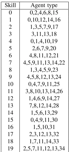
Skill Agent type 0 0,2,4,6,8,15 1 0,10,12,14,16 2 1,3,5,7,9,17

3 3,11,13,18

4 0,1,4,10,19 5 2,6,7,9,20 6 4,8,11,12,21 7 4,5,9,11,13,14,22 8 1,3,4,5,9,23 9 4,5,8,12,13,24 10 0,4,7,9,11,25 11 3,8,10,13,14,26 12 1,4,6,9,14,27 13 7,8,12,14,28 14 1,5,6,13,29 15 0,4,9,11,30

16 1,5,10,31

17 2,3,12,13,32 18 1,7,11,14,33 19 2,5,7,11,12,13,34

Table 1: Each line of the table lists the agents types that can handle a given call type. The skill set of each agent type can be easily inferred. The numbering in the table is started from 0 instead of 1, for compatibility with the simulation and optimization software.

median costs of all solutions (feasible or not) obtained by this method over the 8 independent trials;P∗is the percentage of trials that returned a feasible solution for (SP0n∗); and P₁∗ is the percentage that returned a feasible solution with cost within 1% of the best known feasible solution (the lowest-cost feasible solution for (SP0n∗) generated by either algorithm, over all replications and CPU time budgets).

Algo n n0 min median P1∗ P

∗

cost cost

CP-LP 300 20 136.2 137.5 50 50

TS 1500 156.1 156.1 0 100

Table 2: Empirical results for the example

solution, whose cost is 136.2, was one of the two with worst-case SL of 0.797. In practice, a manager might be willing to use this almost-feasible solution, considering the fact that the center will always experience stochastic variation in the arrival process and the SL in any case. For this reason, it could be useful to report slightly infeasible solutions in general, and not only the feasible ones. All the solutions returned by TS were declared feasible, but they are significantly more expensive, with a cost of 156.1. This shows that large suboptimality gaps with the TS method do occur in realistic call center settings, and not only in artificial examples. We repeated this experiment with a 10-hour CPU budget (n0was doubled andnwas increased to 400 for CP-LP), and none of the two algorithms found a better solution than with the 5-hour budget.

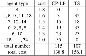
Table 3 summarizes the empirical optima found by CP-LP and by TS. The agent types are regrouped by cost (number of skills). The table gives the total number of agents of each group (each cost) in the solution. We see that CP-LP selects a larger number of agents than TS, but less expensive ones, whence the lower cost.

agent type cost CP-LP TS

4 1.8 0 1

1,5,9,11,13 1.6 3 32

7,12,14 1.5 15 18

0,2,3,8 1.4 19 33

6,10 1.3 23 23

15,. . .,34 1.0 55 0

total number 115 107

total cost 138.8 156.1

Table 3: A summary of the best feasible solutions found by CP-LP and by TS

We also made experiments with other variants of this prob-lem, e.g., with a larger variety of shifts or with fewer periods, and also with other (smaller) problems, and the results were similar. For the smaller problems, the gap between CP and TS was generally smaller (this should depend mostly on the structure of the problem more than its size), but TS was always dominated by CP. We also implemented a meta-heuristic method based on neighborhood search combined with queueing approximation, along the lines of Avramidis et al. (2006), but we were unable to make it competitive with CP for solving (P0).

CONCLUSION

We have proposed in this paper a simulation-based method-ology to optimize agent’s scheduling over one day in a mul-tiskill call center. Even though the use of common random numbers reduces the simulation noise (or variance) signif-icantly, there is still randomness in the solution provided

by the algorithm, mainly due to the fact that the simula-tion lengths must be kept short (because the estimasimula-tion of each subgradient requires simulations at up to thousands of different parameter values). Yet, our approach finds better solutions than with any other method that we know. In prac-tice, one may run the algorithm a few times (e.g., overnight) and retain the best solution found. Future research on this problem include the search for faster ways of estimating the subgradients, refining the algorithm to further reduce the noise in the returned solution, e.g., by improving the way we round non-integer solutions, and extending the technique to simultaneously optimize the scheduling and the routing of calls (via dynamic rules).

ACKNOWLEDGMENTS

This research has been supported by Grants OGP-0110050, OGP38816-05, and CRDPJ-320308 from NSERC-Canada, and a grant from Bell Canada via the Bell University Lab-oratories, to the second and third authors, and a Canada Research Chair to the third author. The fourth author bene-fited from the support of the University of Calabria and the Department of Electronics, Informatics and Systems (DEIS), and her thanks also go to professors Pasquale Legato and Roberto Musmanno. The paper was written while the third author was at IRISA, in Rennes, France.

REFERENCES

Atlason J.; Epelman M.A.; and Henderson S.G., 2004.Call center staffing with simulation and cutting plane methods. Annals of Operations Research, 127, 333–358.

Avramidis A.N.; Chan W.; and L’Ecuyer P., 2006. Staffing multi-skill call centers via search methods and a perfor-mance approximation. Submitted.

Avramidis A.N.; Deslauriers A.; and L’Ecuyer P., 2004. Modeling Daily Arrivals to a Telephone Call Center. Management Science, 50, no. 7, 896–908.

Bhulai S.; Koole G.; and Pot A., 2007. Simple methods for shift scheduling in multi-skill call centers. Man-uscript, available at http://www.cs.vu.nl/∼koole/ research.

Brown L.; Gans N.; Mandelbaum A.; Sakov A.; Shen H.; Zeltyn S.; and Zhao L., 2005. Statistical Analysis of a Telephone Call Center: A Queueing-Science Perspective. Journal of the American Statistical Association, 100, 36– 50.

Cez¸ik M.T. and L’Ecuyer P., 2007. Staffing Multiskill Call Centers via Linear Programming and Simulation. Man-agement Science, 53. To appear.

De-cision CRTC 2000-24. Seehttp://www.crtc.gc.ca/ archive/ENG/Decisions/2000/DT2000-24.htm. Gans N.; Koole G.; and Mandelbaum A., 2003. Telephone

Call Centers: Tutorial, Review, and Research Prospects. Manufacturing and Service Operations Management, 5, 79–141.

Halfin S. and Whitt W., 1981.Heavy-traffic limits for queues with many exponential servers.Operations Research, 29, 567–588.

Henderson S. and Mason A., 1998. Rostering by iterating integer programming and simulation. InProceedings of the 1998 Winter Simulation Conference. vol. 1, 677–683. Ingolfsson A.; Cabral E.; and Wu X., 2003. Combining Integer Programming and the Randomization Method to Schedule Employees. Tech. rep., School of Business, Uni-versity of Alberta, Edmonton, Alberta, Canada. Preprint. Keith E.G., 1979.Operator scheduling.AIIE Transactions,

11, no. 1, 37–41.

Koole G. and Mandelbaum A., 2002. Queueing models of call centers: An introduction. Annals of Operations Research, 113, 41–59.

L’Ecuyer P., 2004. SSJ: A Java Library for Stochastic Simulation. Software user’s guide, Available at http: //www.iro.umontreal.ca/∼lecuyer.

L’Ecuyer P.; Simard R.; Chen E.J.; and Kelton W.D., 2002. An Object-Oriented Random-Number Package with Many Long Streams and Substreams.Operations Research, 50, no. 6, 1073–1075.

Mehrotra V., 1997.Ringing Up Big Business.ORMS Today, 24, no. 4, 18–24.

Pot A.; Bhulai S.; and Koole G., 2007. A simple staffing method for multi-skill call centers. Manuscript, available athttp://www.cs.vu.nl/∼koole/research. Stolletz R. and Helber S., 2004. Performance Analysis of

an Inbound Call Center with Skill-Based Routing. OR Spectrum, 26, 331–352.

Thompson G.M., 1997. Labor staffing and scheduling models for controlling service levels. Naval Research Logistics, 8, 719–740.

Vogel S., 1994. A Stochastic Approach to Stability in Stochastic Programming.Journal of Computational and Applied Mathematics, 56, 65–96.

AUTHOR BIOGRAPHIES

ATHANASSIOS (THANOS) N. AVRAMIDIS is Re-searcher in the D´epartement d’ Informatique et de Recherche Op´erationnelle at the Universit´e de Montr´eal, Canada. He has been on the faculty at Cornell University and a consul-tant with SABRE Decision Technologies. His primary research interests are Monte Carlo simulation, particu-larly efficiency improvement, the interface to probability and statistics, and applications in computational finance,

call center operations, and transportation. His recent re-search articles are available on-line from his web page:

http://www.iro.umontreal.ca/∼avramidi.

MICHEL GENDREAU is Professor of Operations Re-search at Universit´e de Montr´eal, Canada. He is also the Director of the Center for Research on Transportation, a cen-ter devoted to multi-disciplinary research on transportation and telecommunications networks, since 1999. His main research interests deal with the development of exact and approximate optimization methods for transportation and telecommunications network planning problems, topics on which he has published more than 125 papers. Dr. Gen-dreau is the Area Editor of “Heuristic Search and Learning” for the INFORMS Journal on Computing and an Associate Editor of Operations Research, Transportation Science, the Journal of Heuristics, RAIRO-Recherche op´erationnelle and the Journal of Scheduling. He is Vice-President of the In-ternational Federation of Operational Research Societies (IFORS) and Vice-President International of the Institute for Operations Research and the Management Sciences (INFORMS). He received in 2001 the Merit Award of the Canadian Operational Research Society.

PIERRE L’ECUYER is Professor in the D´epartement d’Informatique et de Recherche Op´erationnelle, at the Uni-versit´e de Montr´eal, Canada. He holds the Canada Research Chair in Stochastic Simulation and Optimization. His main research interests are random number generation, quasi-Monte Carlo methods, efficiency improvement via variance reduction, sensitivity analysis and optimization of discrete-event stochastic systems, and discrete-discrete-event simulation in general. He is currently Associate/Area Editor for ACM Transactions on Modeling and Computer Simulation, ACM Transactions on Mathematical Software, Statistical Com-puting, International Transactions in Operational Research, The Open Applied Mathematics Journal, and Cryptography and Communications. He obtained the E. W. R. Steacie fellowship in 1995-97, a Killam fellowship in 2001-03, and he was elected INFORMS Fellow in 2006. His recent research articles are available on-line from his web page:

http://www.iro.umontreal.ca/∼lecuyer.