A moving IRBFN-based integration-free meshless method

Phong B.H. Le1, Timon Rabczuk2Nam Mai-Duy1and Thanh Tran-Cong1

Abstract: A novel approximation method using integrated radial basis function networks (IRBFN) coupled with moving least square (MLS) approximants, namely moving integrated radial basis

function networks (MIRBFN), is proposed in this work. In this method, the computational

do-main Ωis divided into finite sub-domains ΩI which satisfy point-wise overlap condition. The

local function interpolation is constructed by using IRBFN supported by all nodes in subdomain

ΩI. The global function is then constructed by using Partition of Unity Method (PUM), where

MLS functions play the role of partition of unity. As a result, the proposed method is locally

supported and yields sparse and banded interpolation matrices. The computational efficiency are

excellently improved in comparison with that of the original global IRBFN method. In addition,

the present method possesses the Kronecker-δ property, which makes it easy to impose the

essen-tial boundary conditions. The proposed method is applicable to randomly distributed datasets and

arbitrary domains. In this work, the MIRBFN method is implemented in the collocation of a first-order system formulation [Le, Mai-Duy, Tran-Cong, and Baker (2010)] to solve PDEs governing

various problems including heat transfer, elasticity of both compressible and incompressible

ma-terials, and linear static crack problems. The numerical results show that the present method offers high order of convergence and accuracy.

Keywords: RBF, Local IRBF, Moving IRBF, meshless, collocation method, elasticity, first order system, locking, crack.

1 Introduction

Meshless methods have been increasingly used since they provide solutions more continuous than

the piece-wise continuous ones obtained by the finite element methods (FEM). Several meshless methods have been developed, for example, meshless collocation methods [Atluri, Liu, and Han

1_{CESRC, University of Southern Queensland, Toowoomba, QLD 4350, Australia.}

(2006); Libre, Emdadi, Kansa, Rahimian, and Shekarchi (2008)], global weak form meshless

methods [Belytschko, Lu, and Gu (1994)], and local weak form meshless method [Atluri and

Shen (2002); Han and Atluri (2003); Li, Shen, Han, and Atluri (2003)]. In recent years, RBF-based meshless methods have received increasing interest from the research community since the

associated discretisation of the governing PDEs is very simple for random point distribution and

arbitrary domain. Furthermore, global RBFN/IRBFN enjoys spectral accuracy and exponential convergence [Madych (1992); Cheng, Golberg, Kansa, and Zamitto (2003)]. However, the main

drawback of the globally supported RBFN/IRBFN is that the resultant interpolation matrix is dense and highly ill-conditioned due to the nature of global approximation. For example, the condition

number of such a matrix is about 6_×1019with only 20_×20 collocation points [Fasshauer (1997)].

Therefore, globally supported RBFN/IRBFN methods are less effective in large-scale computation and in problems concerning with small-scale features such as cracks/strain localization. Attempts

to deal with this deficiency include domain decomposition method [Ling and Kansa (2004)], block

partitioning and multizone methods [Kansa and Hon (2000)], and preconditioned methods [Baxter (2002); Brown, Ling, Kansa, and Levesley (2005)].

Recently, local RBFN methods have been developed as an alternative approach. Compactly sup-ported RBF truncated from polynomials can improve the condition number, yet a large support

is required to obtain a reasonable accuracy [Wendland (1995)]. It is thus considered not a robust

method against non-uniform datasets [Tobor, Reuter, and Schlick (2004)]. Moreover, some new lo-cal methods that exchange spectral accuracy for a sparse and better-conditioned system, have been

proposed, including explicit local RBF [Šaler and Vertnik (2006)], finite difference based local RBF [Wright and Fornberg (2006); Liu, Zhang, Li, Lam, and Kee (2006)], differential quadrature

based local RBF [Shu, Ding, and Yeo (2003); Shu and Wu (2007)], and radial point interpolation

method [Liu, Liu, and Tai (2005); Liu, Zhang, and Gu (2005)].

Another approach to local RBF is one based on the partition of unity (PU) method. The PU concept

was first introduced by Sherpard and known as Sherpard’s method. However, Sherpard’s method is not widely applied since it is only of constant precision. Since the works of Babuška and Melenk

(1997), this method has received more attention and may be considered an underlying concept

for many other methods such as, PUFEM [Melenk and Babuška (1996)], XFEM [Moës, Dolbow, and Belytschko (1999); Bordas, Duflot, and Le (2008)], GFEM [Strouboulis, Babuška, and Copps

RBF based on the PU concept was first introduced in data fitting by Wendland (2002) and has

been further expanded by several researchers [Tobor, Reuter, and Schlick (2004, 2006); Ohtake,

Belyaev, and Seidel (2006)]. In recent times, the idea of local RBF based on the PU concept was extended by Chen, Hu, and Hu (2008) for solving PDEs. In their method, the reproducing kernel

function is employed as PU function to achieve a higher precision than that of Sherpard method.

Motivated by the former works, this paper proposes a new locally supported MIRBFN method,

in which the standard globally supported IRBFN is coupled with the moving least square (MLS) approximants via the PU concept to formulate a locally supported MIRBFN interpolation method.

Moreover, the present interpolation method is implemented in the collocation of a first-order

sys-tem formulation, resulting in an integration-free meshless method for solving PDEs. The proposed method is verified by various numerical examples, including heat transfer, elasticity of

compress-ible and incompresscompress-ible materials, and linear static crack problems. The remaining of this paper is

organized as follows. The construction of the present MIRBFN is presented in section 2 followed by the first-order system formulation in section 3. Section 4 reports the numerical experiments

and section 5 draws some conclusions.

2 Construction of Moving IRBFN

2.1 The global IRBFN approximation

In the IRBFN method [Mai-Duy and Cong (2001, 2005); Mai-Duy, Khennane, and Tran-Cong (2007); Le, Mai-Duy, Tran-Tran-Cong, and Baker (2007, 2008); Mai-Duy and Tran-Tran-Cong (2009)],

the formulation of the problem starts with the decomposition of the highest order derivatives under

consideration into RBFs. The derivative expressions obtained are then integrated to yield expres-sions for lower order derivatives and finally for the original function itself. The present work is

illustrated with the approximation of a function and its derivatives of order up to 2, the formulation

can be thus described as follows.

u,j j(x) = m

∑

i=1

w(i)g(i)(x), (1)

u,j(x) =

Z m

∑

i=1

w(i)g(i)(x)dxj+C1(xl;l6=j) = m+p1

∑

i=1

w(i)H_[x(i)_j](x), (2)

u(x) =

Z m+p1

∑

i=1

w(i)H(i)(x)dxj+C2(xl;l6=j) = m+p2

∑

i=1

or in compact form

u,j j(x) =G(x)w[xj], (4)

u,j(x) =H[xj](x)w[xj], (5)

u(x) =H_[xj](x)w_[xj], (6)

where, the comma denotes partial differentiation, m is the number of RBFs,_{g(i)(x)_}m

i=1is the set

of RBFs, _{w(i)_}m+p2

i=1 is the set of corresponding network weights to be found, {H(i)(x)}mi=1 and

{_H¯(i)_(x)}m

i=1 are new basis functions obtained by integrating the radial basis function g(i)(x), p1

and p2 are the number of centers used to represent integration constants in the first and second

derivatives, (2) and (3), respectively (p2=2p1). For the multiquadric function

g(i)(x) =qx₋c(i)2+ a(i)2, (7)

where c(i)is the RBF center and a(i)is the RBF width, the width of the ithRBF can be determined

according to the following simple relation

a(i)=βd(i), (8)

whereβ is a factor,β >0, and d(i)is the distance from the ith center to its nearest neighbour.

Now, the “constants” of integration C1(xl;l6=j)and C2(xl;l6=j)on the right hand side of (2) and (3)

can also be interpolated using the IRBFN method as follows.

C′′₁(xl; l6=j) = M

∑

i=1

¯

w(i)g(i)(xl; l6=j), (9)

C1′(xl; l6=j) = M

∑

i=1

¯

w(i)H(i)(xl; l6= j) +Cb1, (10)

C1(xl; l6=j) = M

∑

i=1

¯

w(i)H¯(i)(xl; l6= j) +Cb1xk;k6=j+Cb2, (11)

where_{w¯(i)_}M_i=1are the corresponding weights; M is the number of distinct centers. The unknowns

to be found are the sets of weights in (1) and (9), which can be determined by the SVD (singular

Following Mai-Duy and Tran-Cong (2005), we perform a prior conversion of the unknowns from

network weights, i.e. _{w(i)_}m+p2

i=1 , to nodal function value u in order to form a square system of

equations of smaller size as follows.

The set of network weights are expressed in terms of nodal function value as

w[x]=

H[x]

−1

u, (12)

w[y]=H[y]−

1

u, (13)

and the substitution of (12) and (13) into the system (4)-(6) yields

u,xx(x) =G(x)H[x]

−1

u, (14)

u,x(x) =H[x](x)

H_[x]−1u, (15)

u(x) =H_[x](x)H_[x]−1u, (16)

u,yy(x) =G(x)H[y]

−1

u, (17)

u,y(x) =H[y](x)

H_[y]−1u, (18)

u(x) =H_[y](x)H_[y]−1u, (19)

where I is the identity matrix. It can be seen from (14)-(19) that the function and its derivatives

are all expressed in terms of the function values rather than network weights. Consequently, the system of equations obtained is normally square and the unknowns to be solved for are the nodal

function values instead of the network weights.

2.2 Moving least-square approximants

The moving least-square (MLS) procedure presented in Belytschko, Lu, and Gu (1994) is briefly

reproduced in this section as follows. The interpolant uh_{(x)of the function u(x)is defined in the}

domainΩby

uh(x) =

M

∑

j=1

aj(x)pj(x)≡pT(x)a(x), (20)

a(x)is obtained at any point x by minimizing the following weighted, discrete L2norm

J=

n

∑

I=1

w(x₋xI)[pT(xI)a(x)−uI]2, (21)

where n is the number of points in the neighbourhood of x for which the weight function w(x₋

xI)6=0, and uI is the nodal value of u at x=xI.

The minimization of J in (21) with respect to a(x)leads to the following linear relation between

a(x)and the vector of local nodal values u

A(x)a(x) =B(x)u, (22)

or

a(x) =A−1(x)B(x)u, (23)

where A(x)and B(x)are defined by

A(x) =

n

∑

I=1

w(x₋xI)p(xI)pT(xI) (24)

B(x) =

 

w(x₋x1)

   1 x1 y1  

,w(x₋x2)

   1 x2 y2  

, . . . ,w(x₋xn)

   1 xn yn       (25)

uT= [u1,u2, . . . ,un]. (26)

Substitution of (23) into (20) yields

uh(x) =

n

∑

∑

pj(x)(A−1(x)B(x))jIuI ≡ n

∑

I=1

ϕI(x)uI, (27)

where the shape functionϕI(x)is defined by

ϕI(x) = M

∑

j=1

or in compact form

ϕI(x) =cT(x)w(x−xI)p(xI), (29)

where A(x)c(x) =p(x)defines vector c(x).

c(x) can efficiently be computed by the LU factorization of A(x) with backward substitution

[Belytschko, Krongauz, Fleming, Organ, and Liu (1996); Nguyen, Rabczuk, Bordas, and Duflot

(2008)] as follows.

LUc(x) =p(x), Uc(x) =L−1p(x), c(x) =U−1L−1p(x). (30)

The partial derivatives ofϕI(x)can be obtained by

ϕI,i(x) =cT,i(x)w(x−xI)p(xI) +cT(x)w,i(x−xI)p(xI), (31)

where(.),i= ∂_∂(.)_xi and

c,i(x) =A−,i1(x)p(x) +A−1(x)p,i(x), (32)

with

A,i(x) = n

∑

I=1

w,i(x−xI)p(xI)pT(xI). (33)

It is noted that the following circular kernel function [Schilling, Caroll, and Al-Ajlouni (2001)] is used to compute the present MLS shape function

w(r) =

(

[1+cos(π r

Rs)]/2rα, r

Rs ≤1, α even,

0, r

Rs >1,

(34)

where Rs is the radius of the support domain of the weight function w(r), r=kx−xIkand k.k

2.3 Moving IRBFN interpolation

We propose a locally supported IRBFN, constructed by using the partition of unity concept

[Me-lenk and Babuška (1996); Babuška and Me[Me-lenk (1997)] as follows.

Let the open and bounded domain of interestΩ_⊆Rd_{be discretised by a set of N points}X

X _{={x1,x2, . . . ,xN}, xI∈}Ω, _{I=1,2, . . . ,N, (35)}

X _{is used to define an open cover of} Ω_{, i.e. {}Ω_{I}such that}Ω_⊆SN_I=1Ω_{I and {}Ω_{I}satisfies a}

point-wise overlap condition

∀x_∈Ω _∃k_∈N _{: card{I|x∈}Ω_{I} ≤k. (36)}

We choose a family of compactly supported, non-negative, continuous functionsψI supported on

the closure ofΩI, such that at every point x we have the following property

N

∑

I=1

ψI(x) =1, ∀x∈Ω, (37)

where_{ψI}is called a partition of unity subordinate to the cover{ΩI}.

For every subdomainΩI, a local approximation uI is constructed by using IRBFN supported by

all nodes inΩI as presented in section 2.1, i.e.

uh_I(x)_∈VI, VI=span{H (1) I (x),H

(2)

I (x), . . . ,H (M)

I (x)}, (38)

where{VI}are referred to as the local approximation spaces.

The global approximation of u(x), uh(x)is obtained via

uh(x) =

N

∑

I=1

ψI(x)uhI(x), uh(x)∈V, (39)

whereψI(x)and uhI(x) are associated with the subdomainΩI, and V is called PU method space

and defined by

V :=

N

∑

I=1

In the present work, the partition of unity functionψI is chosen to be identical to the MLS shape

functionϕIin (27), the subdomainΩIis centered at xIas shown in Figure 1.

ReplacingψIwith MLS shape functionϕI, (39) can be rewritten as follows.

uh(x) =

N

∑

I=1

ϕI(x)uhI(x), (41)

and the associated derivatives of uh(x)are given by

uh_,x(x) =

N

∑

I=1

h

ϕI,x(x)uhI(x) +ϕI(x)uhI,x(x)

i

, (42)

uh_,y(x) =

N

∑

I=1

h

ϕI,y(x)uhI(x) +ϕI(x)uhI,y(x)

i

, (43)

where uh_I,x(x)and uh_I,y(x), are derived in (15) and (18).

uh(x)and its derivatives can be rewritten in a compact form as

uh(x) =

N

∑

I=1

ϕI(x)uhI(x) =ΦT(x)u, (44)

uh_,x(x) =ΦT_x(x)u, (45)

uh_,y(x) =ΦT_y(x)u, (46)

where u=_{u1,u2, . . . ,uN},Φ(x)is the vector of shape functions.

It is noted thatΦI(xJ) =δIJ as shown in Figures 3. Consequently, this MIRBFN method

pos-sesses the Kronecker-δ property which makes it easy to impose the essential boundary conditions.

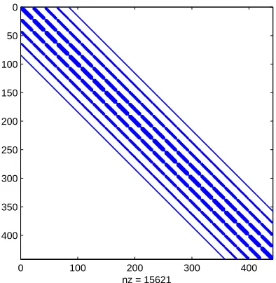
Owing to the locally supported property, MIRBFN yields symmetric, sparse and banded

interpo-lation matrices as shown in Figure 2. This feature makes the method very efficient in storage and computation.

2.4 Selection of RBF centers and support radius

In the present MIRBFN method, the selection of local RBF centers_{ci}_I is very flexible.

Gener-ally, they can be different from the set of local data points{xi}I associated with subdomain ΩI.

For example, if a two-dimensional IRBFN is used, the size of the matrices to be inverted H_[x]and

mI the number of RBF centers {ci}I and p2I the number of centers used to represent integration

constants in the second derivatives. Therefore, the number of columns of the matrices will be p2I

larger than the number of rows when{ci}I is the same as{xi}I. To obtain square matrices, we

choose the number of centers to be less than the number of data points (mI <nI) and p2I to be

appropriately small.

On the other hand, the selection of support radius for each subdomainΩIalso affects the numerical

results significantly. The larger support radius is, the higher accuracy and convergence rate are. However, the higher cost of storage and computation, and the deterioration of the condition number

of the matrices are consequential trade-offs. Hence, to make the method more local and efficient,

smaller values of support radius are preferred in this work.

3 First-order system formulation

For the sake of completeness, the first-order system formulation, which was proposed in a previous

work of the authors [Le, Mai-Duy, Tran-Cong, and Baker (2010)], is reproduced briefly as follows. It is noticed that in general higher-order differential equations can be transformed into a system of

first-order differential equations by introducing some new dual variables, which is the procedure

followed here. Both primary and dual variables are then independently interpolated and have the shape functions of the same order. The resultant first-order system of governing equations can be

written as follows.

L_{u=f, in} Ω ₍₄₇₎

Bu=g, on Γ (48)

whereΩis a bounded domain inRd_{, d=1,2,3,} Γ_{the boundary of}Ω_, L _{is a first-order linear}

differential operator

L_u=L_0u+ d

∑

i=1

L_i∂u

∂xi

, (49)

in which uT = [u1,u2, ...,um]is a vector of m unknown functions (including primary and dual

variables) of xT = [x1,x2, ...,xd], Li the coefficient matrices which characterize the differential

operator L_{, f a given function in the domain, B a boundary algebraic operator, and g a given}

Substituting a discrete approximation of u and its first-order derivatives as given, respectively, in

(41) and (42)-(43) into (47) and (48), and using the collocation method at all the nodes ofΩand

Γ, one obtains a linear algebraic system as presented below.

Let NΩ denote the number of interior nodes, ND the number of nodes on the Dirichlet

bound-ary, NN the number of nodes on the Neumann boundary, mp the number of primary unknowns

and md the number of dual unknowns associated with a node, the number of nodal unknowns

is generally (NΩ+ND+NN)(mp+md). The governing equation (47) is collocated at all the

in-terior and boundary nodes, yielding (N_Ω+ND+NN)(mp+md) equations. The boundary

con-ditions are imposed by collocating (48) at all the boundary nodes, i.e. the obtained system has

(NΩ+ND+NN)(mp+md)+NDkD+NNkNequations, where kDand kNare the number of equations

from the boundary conditions per node on the Dirichlet and Neumann boundaries, respectively.

The final system is obtained by removing NDkD+NNkN appropriate equations corresponding to

the governing equations collocated at the boundary nodes. Consequently, the number of equations of the resultant system is equal to the number of nodal unknowns and it can be rewritten in a

compact form as

Au=¯f. (50)

3.1 Two-dimensional Poisson equation

Consider the following two-dimensional Poisson equation

∂2φ(_x,y) ∂x2 +

∂2φ_(x,y)

∂y2 = f(x,y) in Ω, (51a)

φ(x,y) =g(x,y) on ΓD, (51b)

∂φ(x,y)

∂n =h(x,y) on ΓN, (51c)

whereΩis a bounded domain inR2_, Γ

Dand ΓN the boundary ofΩon which the Dirichlet and

Neumann boundary conditions are imposed, respectively, n= (nx,ny)T the outward unit normal

A first-order formulation is obtained by introducing the dual variables in (51) as follows.

∂φ(x,y)

∂x −ξ(x,y) =0 in Ω and on ΓD

[

ΓN, (52a)

∂φ(x,y)

∂y −η(x,y) =0 in Ω and on ΓD

[

ΓN, (52b)

∂ξ(x,y) ∂x +

∂η(x,y)

∂y = f(x,y) in Ω and on ΓD

[

ΓN, (52c)

φ(x,y) =g(x,y) on ΓD, (52d)

nxξ+nyη=h(x,y) on ΓN. (52e)

3.2 Linear elasticity problems

Consider the following two-dimensional problem on a domainΩbounded byΓ=ΓuSΓt

∇·σ=b in Ω, (53a)

u=¯u on Γu, (53b)

σ·n=¯t on Γt, (53c)

in whichσ is the stress tensor, which corresponds to the displacement field u and b is the body

force, n the outward unit normal toΓt. The superposed bar denotes prescribed value on the

bound-ary.

The governing equations (53) are closed when a constitutive relation is specified forσ. Here the

linear Hooke’s law is used to describe theσ₋u relation. By choosing displacement u as primary

for plane stress case as follows.

∂u

∂x− 1 Eσx+

µ

Eσy=0, (54a)

∂v

∂y+

µ

Eσx− 1

Eσy=0, (54b)

∂u

∂y+

∂v

∂x−

2(1+µ)

E τxy=0, (54c)

∂σx

∂x +

∂τxy

∂y =bx, (54d)

∂τxy

∂x +

∂σy

∂y =by, (54e)

u=¯u on Γu, (54f)

σ·n=¯t on Γt, (54g)

whereµ is the Poisson ratio and E the Young’s modulus. By introducing the dimensionless stress

tensor s=σ/E, the above first-order system can be rewritten as follows.

∂u

∂x−sx+µsy=0, (55a)

∂v

∂y+µsx−sy=0, (55b)

∂u

∂y+

∂v

∂x−2(1+µ)sxy=0, (55c)

∂sx

∂x +

∂sxy

∂y =bx, (55d)

∂sxy

∂x +

∂sy

∂y =by, (55e)

u=¯u on Γu, (55f)

4 Numerical examples

For an error estimation and convergence study, the discrete relative L2 norm of errors of primary

and dual variables are defined as

Lφ₂ =

r

∑N i=1

φ(i) e −φ(i)

2 r ∑N i=1 φ(i) e

2 , (56)

Lξη₂ =

s

∑N i=1

ξ(i) e −ξ(i)

2

+ηe(i)−η(i)

2 s ∑N i=1 ξ(i) e 2

+ηe(i)

2

, (57)

for Poisson equation and

Lu₂=

r

∑N i=1

(ux)(i)e −(ux)(i)

2

(uy)(i)e −(uy)(i)

2

s

∑N i=1

(ux)(i)e

2

+(uy)(i)e

2

, (58)

Lσ₂ =

s

∑N i=1

(sx)(i)e −s(i)x

2

+(sy)(i)e −s(i)y

2

+(sxy)(i)e −s(i)xy

2

s

∑N i=1

(sx)(i)e

2

+(sy)(i)e

2

+(sxy)(i)e

2

, (59)

for elasticity problems, where N is the number of unknown nodal values and the subscript “e" denotes the exact solution. The convergence order of the solution with respect to the refinement

of spatial discretization is assumed to be in the form of

L2(h)≈ζhλ=O(hλ), (60)

where h is the maximum nodal spacing, ζ and λ are the parameters of the exponential model,

which are found by general linear least square formula in this work.

GB of RAM and two Intel(R) Xeon(R) CPUs of 3.0 GHz each. The code is written in MATLABr

language.

4.1 Poisson equation

4.1.1 Poisson equation in a regular domain

Consider the following Poisson equation

∂2_φ(x,y) ∂x2 +

∂2_φ(x,y)

∂y2 =−2π

2_{cos(πx)cos(πy), (61)}

defined inΩ= [0,1]_×[0,1], subjected to the Dirichlet boundary condition

φ(0,y) =cos(πy), on x=0, (62)

and the following Neumann boundary conditions

∂φ(1,y)

∂x =0, on x=1, (63a)

∂φ(x,0)

∂y =0, on y=0, (63b)

∂φ(x,1)

∂y =0, on y=1. (63c)

(63d)

The corresponding exact solution is given by

φ(x,y) =cos(πx)cos(πy). (64)

Two discretisations are considered for this problem: uniform and nonuniform distributions of

nodes/collocation points (CPs) as shown in Figures 4 and 8, respectively. For both cases, the

radius of support domains is set atRs_h =2.1, where h is the maximum spacing between two nearest

nodes in x or y direction. The maximum number of uniformly distributed RBF centers mI in each

subdomain is 5 as shown in Figure 4. The numbers of centers to represent the integration constants

p1I and p2I are 3 and 6, respectively. The values ofβ in (8) for both cases are listed in Tables 1

Table 1: Poisson equation in a regular domain: uniform discretisations with MIRBFN

No. points Lφ₂ Lξη₂ cond(A) β Rs_h CPU time_second

3_×3 0.4415 1.1413 51.7250 12 2.1 0.15

7_×7 0.0252 0.0219 512.8116 12 2.1 0.30

11_×11 0.0036 0.0041 813.8110 12 2.1 0.59

21_×21 4.4864e-4 5.5402e-4 2.2514e3 12 2.1 2.07

25_×25 2.5203e-4 3.1671e-4 2.9034e3 12 2.1 3.07

31_×31 1.2419e-4 1.5922e-4 4.1964e3 12 2.1 5.13

41_×41 5.0132e-5 6.5620e-5 6.1935e3 12 2.1 10.59

61_×61 1.4217e-5 1.9006e-5 1.5362e4 12 2.1 35.84

81_×81 5.9951e-6 8.0377e-6 3.5862e4 12 2.1 90.0

91_×91 4.2892e-6 5.6966e-6 5.2312e4 12 2.1 136.40

101_×101 3.2363e-6 4.2199e-6 7.4923e4 12 2.1 197.11

121_×121 2.1324e-6 2.6352e-6 9.037e4 12 2.1 374.7

O(h3.32) O(h3.38)

Table 2: Poisson equation in a regular domain: uniform discretisations with global IRBFN

No. points Lφ₂ Lξη₂ cond(A) β CPU time_second

7_×7 0.0245 0.0273 1.6043e4 1 0.161

11_×11 0.0038 0.0048 2.5617e4 1 0.179

21_×21 7.4562e-5 1.5070e-4 5.8907e4 1 2.462

31_×31 1.2924e-5 2.3775e-5 1.2225e5 1 30.064

41_×41 4.3906e-6 7.9095e-6 2.0292e5 1 149.319

51_×51 2.1210e-6 3.7691e-6 3.0404e5 1 535.049

61_×61 1.3851e-6 2.1592e-6 7.0649e4 1 1674.980

O(h4.71) O(h4.52)

Table 3: Poisson equation in a regular domain: unstructured nodes with MIRBFN

No. points Lφ₂ Lξη₂ cond(A) β Rs_h h CPU time_second

88 0.2833 0.1438 1.6887e5 10 2.1 0.1250 0.73

108 0.0402 0.0613 4.5345e5 10 2.1 0.1200 0.80

327 0.0077 0.0057 6.2091e7 10 2.1 0.0685 2.23

691 0.0018 0.0019 4.5704e8 10 2.1 0.0507 5.65

1723 7.2107e-4 5.7631e-4 1.3461e8 10 2.1 0.0308 22.12

2248 3.3681e-4 2.5718e-4 1.2765e8 12 2.1 0.0272 35.58

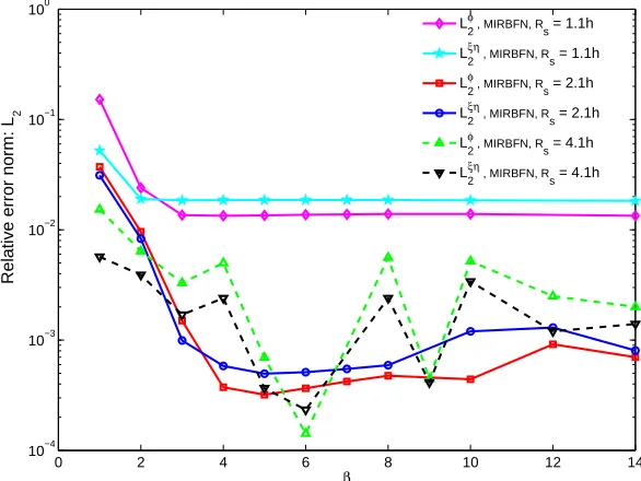
The influences of local support radius Rs_h and β on the accuracy of the solution are numerically

studied in this example. Figure 5 shows the relative error norms (Lφ₂ and Lξη₂ ) obtained by the

present MIRBFN method with different values of Rs_h while β is fixed. On the other hand, the

results with different values ofβ and fixed local support radius are displayed in Figure 6. It can

be seen that the values around 2 for Rs_h are not only able to capture well the solution but also keep

the matrix small, as long asβ is large enough.

To study the convergence of the method, a number of discretization refinements and the relative

L2 error norms for function values Lφ2 and its derivatives L

ξη

2 are reported in Tables 1 and 3 for

uniform and unstructured cases, respectively. As shown in these tables and Figures 7 and 9, very

good accuracy and stability are obtained. The convergence rates forφ(x,y)and (ξ(x,y),η(x,y)) are O(h3.32)and O(h3.38), respectively, for uniform distribution, and, O(h3.78)and O(h3.82), re-spectively, for unstructured nodes. It can be seen that the condition numbers in the case of uniform

distribution are relatively smaller than those in the case of random distribution (Table 3) since there is a relatively larger number of nodes in each subdomain in the case of random distribution.

The results in Tables 1-2 and Figure 7 indicate that the global IRBFN gives higher orders of

convergence. Nonetheless, the condition numbers by the MIRBFN method are slightly better in

comparison with those by the global IRBFN method, as listed in Tables 1 and 2, althoughβ is set

quite large for the MIRBFN method. Furthermore, the MIRBFN method is much more efficient

than the global IRBFN method as can be seen in Figure 10.

4.1.2 Poisson equation in an irregular domain

The Poisson equation in example 4.1.1 is examined in a complicated irregular domain as shown

in Figure 11. The Dirichlet boundary conditions on the upper edge and the left edge are given as

below

φ(0,y) =cos(πy), on x=0, (65a)

Table 4: Poisson equation in an irregular domain: structured dicerizations with MIRBFN

No. points Lφ₂ Lξη₂ cond(A) β Rs_h h CPU time_second

51 3.4762e-1 5.4441e-1 3.1001e5 9 4.1 0.25 0.83

87 2.8487e-2 5.2716e-2 1.9944e6 9 4.1 0.181 1.31

266 1.4620e-3 3.8399e-3 2.0634e7 9 4.1 0.0095 3.86

595 5.0421e-4 8.7207e-4 6.4519e8 9 4.1 0.0065 11.55

1029 1.7279e-4 4.0659e-4 6.2724e8 9 4.1 0.0048 23.05

1574 8.5957e-5 2.4792e-4 4.1291e8 9 4.1 0.039 43.17

2266 3.6035e-5 8.0371e-5 6.5102e9 9 4.1 0.039 84.48

3413 3.0210e-5 5.0281e-5 1.9016e8 9 4.1 0.033 172.53

O(h4.06) O(h3.96)

Table 5: Poisson equation in an irregular domain: unstructured discretisation with MIRBFN

No. points Lφ₂ Lξη₂ cond(A) β Rs_h h CPU time_second

51 1.9465e-1 1.9142e-1 7.5387e4 14 3.1 2.7337e-1 4.775

338 2.4059e-3 6.7564e-3 4.4212e6 14 3.1 1.1182e-1 22.017

1046 7.1240e-4 1.7302e-3 9.0038e6 12 3.1 5.9731e-2 89.633

1486 4.2708e-4 8.4299e-4 7.5913e7 12 3.1 5.3098e-2 203.883

1711 1.4251e-4 2.1264e-4 1.4224e8 8 3.1 4.8722e-2

O(h3.80) O(h3.50)

The Neumann boundary conditions on the inner arc and the outer arc are, respectively

nx

∂φ(x,y) ∂x +ny

∂φ(x,y)

∂y =q(x,y), on x

2_+y2_{=1, (66a)}

nx∂φ( x,y) ∂x +ny

∂φ(x,y)

∂y =q(x,y), on x

2_+y2_{=4, (66b)}

where q(x,y) =₋nxπsin(πx)cos(πy)−nyπcos(πx)sin(πy).

The complexity is increased with the Neumann boundary conditions on two curved boundaries.

The structured domain discretisation is described as follows. A uniformed grid covering the

do-main is generated, then the points outside the dodo-main and on the curves are removed. Finally, the points on the inner and outer arcs are generated uniformly.

In the case of structured discretisation (Figure 11), the local support radius Rs_h is set at 4.1,β is 9,

the maximum number of centers in each subdomain is 13. The relative L2error norms Lφ2 and L

ξη

2

can be observed that high orders of convergence are obtained with a large support radius, namely

O(h4.06) and O(h3.96) for the function and its derivatives, respectively. However, the condition numbers are much larger than those in the previous example. For unstructured node distributions (Figure 12), the corresponding parameters and obtained results are presented in Table 5 and Figure

14. The results indicate that the solution by the proposed method apparently converges at the rates

of (O3.80) and (O3.50), using Lφ₂ and Lξη₂ , respectively.

4.2 Linear elasticity problems

4.2.1 Cantilever Beam

A cantilever beam subjected to a parabolic shear load at the end x=0 as shown in Figure 15 is

considered in this example.

Table 6: Cantilever beam: uniform discretizations with MIRBFN (µ =0.3).

No. points Lu₂ Lσ₂ cond(A) β Rs_h h CPU time_second

20_×5 1.9598e-1 3.3652e-1 4.1516e6 8 2.1 0.240 0.60

36_×9 1.4986e-2 2.5489e-2 1.4193e8 10 2.1 0.133 1.84

68_×17 1.2182e-3 2.1326e-3 3.0383e6 14 2.1 0.070 6.98

124_×31 5.8434e-4 5.7764e-4 4.0336e6 14 2.1 0.039 43.78

164_×41 2.2892e-4 2.3983e-4 8.3453e6 14 2.1 0.029 109.42

204_×51 1.1069e-4 1.2366e-4 14 2.1 0.024 230.01

244_×61 5.9462e-5 7.2455e-5 14 2.1 0.020 438.98

O(h3.04) O(h3.26)

The following parameters are used for the problem: L=4.8 and D=1.2. The beam has a unit

thickness. Young’s modulus is E =3_×106 , Poisson’s ratio µ =0.3 (also µ =0.5) and the

integrated parabolic shear force P=100. Plane stress condition is assumed and there is no body

force.

The exact solution to this problem was given by Timoshenko and Goodier (1970) as

σxx(x,y) = − Pxy

I , (67a)

σyy(x,y) =0, (67b)

τxy(x,y) =− P 2I

D2

4 −y

2

Table 7: Cantilever beam: uniform discretizations with MIRBFN (µ =0.5).

No. points Lu₂ Lσ₂ cond(A) β Rs_h h CPU time_second

20_×5 1.0069e-1 1.9291e-1 2.3672e7 8 2.1 0.240 0.60

36_×9 2.0936e-2 5.3772e-2 4.2607e7 10 2.1 0.133 1.81

68_×17 7.8576e-4 1.6020e-3 2.1090e6 14 2.1 0.070 6.77

124_×31 4.3029e-4 4.1872e-4 2.8678e6 14 2.1 0.039 41.12

164_×41 1.6292e-4 1.6988e-4 5.7418e6 14 2.1 0.029 106.48

204_×51 7.7595e-5 8.7489e-5 14 2.1 0.024 235.5

244_×61 4.1951e-5 5.2041e-5 14 2.1 0.020 475.7

O(h3.07) O(h3.39)

Table 8: Cantilever beam: uniform discretizations with global IRBFN (µ =0.3).

No. points Lu₂ Lσ₂ cond(A) β h CPU time_second

20_×5 4.5356e-2 2.5571e-1 1.7953e6 1 0.2400 0.408

36_×9 5.2822e-3 4.0279e-2 5.2505e6 1 0.1333 2.068

68_×17 1.5706e-3 2.6022e-3 6.5476e7 1 0.0706 68.088

124_×31 3.8901e-4 4.3698e-4 3.1351e8 1 0.0387 2351.78

164_×41 2.1295e-4 2.2075e-4 1 0.0293 51201.338

O(h3.06) O(h3.39)

Table 9: Cantilever beam: unstructured nodes with MIRBFN (µ =0.3).

No. points Lu₂ Lσ₂ cond(A) β Rs_h h CPU time_second

43 6.5385e-1 6.9895e-1 2.6549e6 10 2.1 4.6860e-1 0.715

170 2.7461e-2 5.5154e-2 3.9549e7 10 2.1 2.4000e-1 2.079

616 7.2999e-3 3.1141e-2 7.4558e7 10 2.1 1.2507e-1 7.888

1112 4.9025e-4 3.0318e-3 1.0345e9 10 2.1 1.0454e-1 20.190

O(h4.21) O(h3.07)

Table 10: Cantilever beam: structured FEM mesh with four-node quadrilateral element (Q4) (µ=

0.3).

No. elements Lu₂ h CPU time_second

16×4 1.3991e-1 0.40 0.1806

32_×8 3.8516e-2 0.1714 0.4395

40_×10 2.5191e-2 0.1333 1.7111

80×20 6.9048e-3 0.0631 8.4087

160_×40 1.6994e-3 0.0307 21.5620

240_×60 9.1261e-4 0.0203 47.9957

320_×80 6.1308e-4 0.0152 307.579

The displacements are given by

ux=− Px2y

2EI −

µPy3

6EI +

Py3

6IG+y

PL2

2EI−

PD2 8IG

, (68)

uy=µ Pxy2

2EI +

Px3

6EI−

PL2x

2EI +

PL3

3EI, (69)

where I=D3/12 is the moment of inertia of the cross section of the beam, G=E/(2(1+µ))the

modulus of elasticity in shear. The exact displacement (68) and (69) are imposed on x=L while

the shear load is applied on x=0 and the upper and lower edges are traction free.

Both regular and irregular distributions of nodes used for this problem are displayed in Figures 16

and 18, respectively. The local support radius is Rs_h =2.1. The values ofβ are listed in Tables 6,

7 and 9. The scheme for selection of RBF centers for both regular and irregular node distributions is similar to that in example 4.1.1. In addition, the effect of incompressibility, i.e. µ=0.5, is also

studied here.

Figure 19 shows the shear stress sxyforµ=0.3 at x=2.4686 obtained by the present method with

36_×9 nodes. A very good agreement between the obtained result and the exact solution can be

observed in this figure.

To study the convergence of the method, a number of different uniform node distributions is used

for computation as presented in the Tables 6 and 7. Forµ =0.3, the relative L2error norms for

displacement and stress are shown in Table 6 and Figure 20, the convergence rates of displacement

and stress are O(h3.04) and O(h3.26), respectively. In the case of incompressible materials (µ =

0.5), the relative L2error norms for displacement and stress are presented in Table 7 and Figure 20.

Very good orders of convergence are achieved, namely O(h3.07)and O(h3.39)for displacement and stress, respectively. Furthermore, the results shown in Figure 20 indicate that the present method

does not suffer from any volumetric locking.

The behaviour of the MIRBFN method in the case of irregular discretisation is also examined with

four nodal configurations as shown in Figure 18. The obtained results with the MIRBFN method

andµ=0.3 are shown in Table 9 and Figure 21. The orders of convergence of the present method

are O(h4.21)and O(h3.07)for displacement and stress, respectively.

In comparison with the global IRBFN method, the MIRBFN method achieves similar accuracy

and convergence rates as can be observed in Tables 6 and 8, and in Figure 20 as well. The present

The obtained results are also compared with those by FEM using four-node quadrilateral element

(Table 10). Figure 20 shows that both accuracy and order of convergence of the MIRBFN method

are superior to those of FEM, e.g. using Lu₂, the convergence rates are O(h3.04)and O(h1.84) for the MIRBFN method and the FEM, respectively. The computing cost of the MIRBFN method

is higher than that of the FEM for the same number of nodes. However, the MIRBFN method is

more efficient than the FEM for the same accuracy, for example, it takes the MIRBFN method 6.98 seconds for Lu₂=1.2182_×10−3while the FEM needs 21.56 seconds to achieve Lu₂=1.6994_×10−3

as exhibited in Figure 22, Table 6 and Table 10.

4.2.2 Infinite plate with a circular hole

In this example, an infinite plate with a circular hole subjected to unidirectional tensile load of 1.0 in the x direction is analyzed as shown in Figure 23. The radius of hole is taken as 1 unit. Owing

to symmetry, only the upper right quadrant[0,3]_×[0,3]of the plate is modeled as shown in Figure

24.

In this problem, plane stress conditions are assumed with elastic isotropic properties E =103,

µ =0.3 (alsoµ=0.5). The exact solution to this problem was given by Timoshenko and Goodier

(1970) as follows

σx(x,y) =σ

1₋a

2

r2

3

2cos(2θ) +cos(4θ)

+3a 4

2r4 cos(4θ)

, (70a)

σy(x,y) =−σ

a2 r2

1

2cos(2θ)−cos(4θ)

+3a 4

2r4 cos(4θ)

, (70b)

τxy(x,y) =−σ

a2 r2

1

2sin(2θ) +sin(4θ)

−3a 4

2r4sin(4θ)

, (70c)

where(r,θ)are the polar coordinates, a the radius of the hole.

The corresponding displacements are given by

ux(x,y) =σ

(1+µ)

E

1

1+µr cos(θ) +

2

1+µ

a2

r cos(θ) + 1 2

a2

r cos(3θ)− 1 2

a4

r3cos(3θ)

(71a)

uy(x,y) =σ

(1+µ)

E

−µ

1+µr sin(θ) +

1₋µ

1+µ

a2

r sin(θ) + 1 2

a2

r sin(3θ)− 1 2

a4

r3sin(3θ)

(71b)

cor-Table 11: Infinite plate with a circular hole: structured discretisation with MIRBFN (µ =0.3).

No. points Lu

2 Lσ2 cond(A) β

Rs

h h

CPU time second

50 3.0520e-1 2.6147e-1 6.7532e4 4 2.1 0.50 0.54

119 9.2110e-2 8.1240e-2 8.3533e6 4 2.1 0.30 1.03

409 1.0837e-2 1.2229e-2 6.1059e4 4 2.1 0.15 3.25

1129 8.7872e-4 2.6677e-3 2.0085e5 4 2.1 0.088 10.56

3085 1.8647e-4 4.2703e-4 4.4334e5 4 2.1 0.052 44.36

O(h3.61) O(h3.02)

Table 12: Infinite plate with a circular hole: structured discretisation with MIRBFN (µ =0.5).

No. points Lu₂ Lσ₂ cond(A) β Rs_h h CPU time_second

50 7.8208e-1 5.7769e-1 1.1433e5 4 2.1 0.50 0.54

119 1.0186e-1 8.2598e-2 5.0328e6 4 2.1 0.30 1.01

409 1.3343e-2 1.4314e-2 5.5146e4 4 2.1 0.15 3.20

1129 9.5928e-4 2.7873e-3 2.0372e5 4 2.1 0.088 10.48

3085 4.0203e-4 4.6366e-4 6.0161e5 4 2.1 0.052 43.06

O(h3.68) O(h3.27)

Table 13: Infinite plate with a circular hole: structured discretisation with global IRBFN (µ=0.3).

No. points Lu₂ Lσ₂ cond(A) β h CPU time_second

119 1.3243e-1 1.1085e-1 7.0056e5 1 0.2727 0.413

409 2.3900e-2 1.5925e-2 1.4568e6 1 0.1429 2.222

886 4.8966e-3 3.3027e-3 3.3118e6 1 0.0968 21.323

3085 2.5075e-4 7.2314e-4 4.3415e6 1 0.0517 977.988

O(h3.78) O(h3.08)

responding to the exact solution for the infinite plate are applied on the top and right edges, the symmetric conditions are applied on the left and bottom edges, and the curved edge is traction

free.

To solve the problem, the computational domain is discretized in the same manner as in example

4.1.2. The support radius is Rs_h =2.1, the value ofβ varies between 3 and 4 as in Tables 11, 12

and 14, and the RBF centers are identical to the nodes in each subdomain.

A comparison between the stress sx along x=0 obtained by the MIRBFN with a structured

dis-cretisation of 409 nodes and the exact solution are presented in Figure 26. The result indicates that

Table 14: Infinite plate with a circular hole: unstructured node distribution with MIRBFN (µ =

0.3).

No. points Lu₂ Lσ₂ cond(A) β Rs_h h CPU time_second

68 7.5923e-1 8.0880e-1 4.9714e4 4 2.1 5.0000e-1 1.383

156 2.3616e-1 3.4100e-1 2.9975e5 4 2.1 3.0888e-1 2.911

479 1.0531e-2 4.0582e-2 2.7228e6 4 2.1 1.6343e-1 8.729

1024 5.0684e-3 2.2821e-2 6.2775e6 3 2.1 1.1346e-1 23.620

2439 9.9303e-4 8.2974e-3 1.2450e8 3 2.1 7.5139e-2 81.186

O(h3.60_{) O(h}2.50₎

The convergence of the present method in the case of structured node distribution (Figure 24)

is reported in Table 11 and Figure 27 for µ =0.3, and in Table 12 and Figure 27 for the case

of incompressible materials. The present method appears to converge at the rates of O(h3.61)for

displacement and O(h3.02)for stress in the case ofµ=0.3. In the case of incompressible materials, the orders of convergence are O(h3.68)and O(h3.27)for displacement and stress, respectively. The performance of the MIRBFN method is also tested with irregular node distributions as shown in Figure 25. The obtained results are presented in Table 14 and Figure 28, which show that the

convergence rates are O(h3.60)and O(h2.50)for displacement and stress, respectively.

Again, the MIRBFN method achieves similar accuracy and convergence rates in comparison with

those of the global IRBFN method as shown in Table 11 and 13, and in Figure 27. Clearly, the

efficiency of the present method is superior to that of the global IRBFN (Figure 29).

4.2.3 Mode I crack problem

Consider an infinite plate containing a straight crack of length 2a and loaded by a remote uniform

stress field σ as shown in Figure 30. Along ABCD the closed form solution in terms of polar

coordinates in a reference frame(r,θ)centered at the crack tip is given by

σx= KI √ rcos θ 2

1₋sinθ

2sin 3

θ

2

, (72a)

σy= KI √ rcos θ 2

1+sinθ

2sin 3

θ

2

, (72b)

τy= KI √ rsin θ 2cos θ

2cos 3

θ

Table 15: Center crack problem: uniform discretisations with MIRBFN (µ =0.3).

No. points Lu

2 Lσ2 cond(A) β

Rs

h h

CPU time second

10_×10 0.2017 1.3794 2.7726e5 0.01 1.1 1.0 0.53

14_×14 0.13882 0.6583 6.7641e5 0.01 1.1 0.714 0.94

16_×16 0.0909 0.5043 4.7002e5 0.01 1.1 0.625 1.22

20_×20 0.0374 0.2327 5.1297e5 0.01 1.1 0.50 1.85

24_×24 0.0269 0.1887 1.6910e6 0.01 1.1 0.416 2.68

O(h2.47) O(h2.38)

for stress and

ux=

2(1+µ) √

2π KI

E

√

r cosθ 2

2₋2µ₋cos2θ 2

, (73a)

uy=

2(1+µ) √

2π KI

E

√

r sinθ 2

2₋2µ₋cos2θ 2

, (73b)

for displacement, where KI=σ√πa is the stress intensity factor,µ Poisson’s ratio and E Young

modulus, ABCD a square of 10_×10 mm2, a=100 mm, E=107N/mm2,µ =0.3 (alsoµ=0.5),

σ=104N/mm2. Plane strain condition is assumed and the body force is zero.

The computational domain ABCD is shown in Figure 30. Owing to symmetry, only upper half of ABCD, namely CDEFG as shown in Figure 31, is analyzed. The segment of crack denoted by EF

has a length of b=5 mm. The boundary condition of the problem is as follows. The traction free

boundary condition is applied on the crack while the displacement field given in (73) is imposed on the remaining boundaries.

It is known that stress tends to infinity when r tends to 0. Thus, to alleviate the oscillation due

to the effect of singularity, the support radius Rsand β are selected as small as possible. For this

example, Rs_h and β are set at 1.1 and 0.01, respectively, and the RBF centers are chosen to be

identical to the nodes in each subdomain.

The performance of the present method in this singular problem is examined by employing a number of uniform data point distributions as displayed in the Tables 15 and 16. The results

with 24_×24 nodes (µ =0.3) are plotted in Figures 32-34 as follows. Figures 32 and 33 exhibit

displacement uxand uy, respectively, in comparison with those of an analytical solution. Figures 34

(a) and (b) depict stress sxand syby MIRBFN method, respectively, and the corresponding exact

Table 16: Center crack problem: uniform discretizations with MIRBFN (µ=0.5).

No. points Lu

2 Lσ2 cond(A) β Rsh h

CPU time second

10_×10 0.1087 0.9622 1.4859e5 0.01 1.1 1.0 0.53

14_×14 0.1064 0.6401 2.9922e5 0.01 1.1 0.714 0.94

16_×16 0.0477 0.3233 2.8071e5 0.01 1.1 0.625 1.22

20_×20 0.0366 0.2627 5.3818e5 0.01 1.1 0.50 1.85

24_×24 0.0379 0.2613 4.9657e5 0.01 1.1 0.416 2.73

O(h1.44) O(h1.64)

continuity of displacement and C_∞ property of IRBFNs. This oscillation is known as the Gibbs

phenomenon in RBF-based methods [Jung (2007)] where numerical oscillations occur around a jump discontinuity because of high order approximation by RBF. Nevertheless, the obtained

results are in good agreement with the analytical ones and the present MIRBFN method is able to

capture highly steep gradients.

The convergence of the method can be seen in Tables 15 and 16, and in Figure 35. In the case of

µ=0.3, high convergence rates of O(h2.47)and O(h2.38)for displacement and stress, respectively, are obtained. It is apparent that accuracy of the stress field is considerably reduced in

compari-son with that of displacement due to the presence of singularity (Figure 35,). For incompressible

materials, the convergence rates reduce to O(h1.44)and O(h1.64)for displacement and stress, re-spectively.

5 Concluding remarks

In this work, we propose a locally supported RBF interpolation method, namely MIRBFN, with

the main features as follows.

• The proposed method is a locally supported approximation method. As a result, the resultant

interpolation matrices are sparse and banded, resulting in improved efficiency in comparison

with those of standard RBF methods.

• The shape functions of the MIRBFN method possesses the Kronecker-δ property that

facil-itates the imposition of the essential boundary conditions.

• The present method offers high orders of convergence and is applicable to scattered node

Moreover, the proposed interpolation method is implemented in the collocation of a first-order

sys-tem formulation resulting in an integration-free meshless method which enjoys high convergence

rate and very good accuracy.

Acknowledgement: This work is supported by the Australian Research Council. This support is gratefully acknowledged.

References

Atluri, S.; Shen, S. (2002): The meshless local Petrov-Galerkin (MLPG) method:A simple & less-costly alternative to the finite element and the boundary element methods. CMES: Computer Modeling in Engineering & Sciences, vol. 3, pp. 11–51.

Atluri, S. N.; Liu, H. T.; Han, Z. D. (2006): Meshless local Petrov-Galerkin (MLPG) mixed

col-location method for elasticity problems. CMES: Computer Modeling in Engineering & Sciences, vol. 14, no. 3, pp. 141–152.

Babuška, I.; Melenk, I. (1997): The partition of unity method. International Journal for Numerical Methods in Engineering, vol. 40, no. 4, pp. 727–758.

Baxter, B. (2002): Preconditioned conjugate gradient, radial basis functions, and toeplitz

matri-ces. Compu. Math. Appl., vol. 43, pp. 305–318.

Belytschko, T.; Krongauz, Y.; Fleming, M.; Organ, D.; Liu, W. (1996): Smoothing and accelerated computations in the element-free Galerkin method. J. Comput. Appl. Math, vol. 74, pp. 111–126.

Belytschko, T.; Lu, Y. Y.; Gu, L. (1994): Element-free Galerkin methods. International Journal

for Numerical Methods in Engineering, vol. 37, pp. 229–256.

Bordas, S.; Duflot, M.; Le, P. (2008): A simple error estimator for extended finite elements. Communications In Numerical Methods In Engineering, vol. 24, pp. 961–971.

Brown, D.; Ling, L.; Kansa, E.; Levesley, J. (2005): On approximate cardinal

precondition-ing methods for solvprecondition-ing pdes with radial basis functions. Engineering Analysis with Boundary

Elements, vol. 29, pp. 343–353.

Chen, J.; Hu, W.; Hu, H. (2008): Reproducing kernel enhanced local radial basis collocation method. International Journal for Numerical Methods in Engineering, vol. 75, pp. 600–627.

Fasshauer, G. (1997): Solving partial differential equations by collocation with radial basis functions. In Méhauté, A. L.; Rabut, C.; Schumaker, L.(Eds): Surface Fitting and Multiresolution Methods, pp. 131–138. Vanderbilt University Press.

Han, Z. D.; Atluri, S. N. (2003): Truly meshless local petrov-galerkin (MLPG) solutions of traction & displacement BIEs. CMES: Computer Modeling in Engineering & Sciences, vol. 4, no. 6, pp. 665–678.

Jung, J. H. (2007): A note on the Gibbs phenomenon with multiquadratic radial basis functions.

Applied Numerical Mathematics, vol. 57, pp. 213–229.

Kansa, E.; Hon, Y. (2000): circumventing the ill-conditioning problem with multiquadric radial

basis functions: application to elliptic partial differential equations. Compu. Math. Appl., vol. 39, pp. 123–137.

Le, P.; Mai-Duy, N.; Tran-Cong, T.; Baker, G. (2007): A numerical study of strain localization

in elasto-therno-viscoplastic materials using radial basis function networks. CMC: Computers,

Materials & Continua, vol. 5, pp. 129–150.

Le, P.; Mai-Duy, N.; Tran-Cong, T.; Baker, G. (2008): A meshless modeling of dynamic strain

localization in quasi-britle materials using radial basis function networks. CMES: Computer

Modeling in Engineering & Sciences, vol. 25, no. 1, pp. 43–66.

Le, P.; Mai-Duy, N.; Tran-Cong, T.; Baker, G. (2010): A Cartesian-grid Collocation Technique

with Integrated Radial Basis Functions for mixed boundary value problems. International Journal for Numerical Methods in Engineering, vol. 82, pp. 435–463.

Li, Q.; Shen, S.; Han, Z. D.; Atluri, S. N. (2003): Application of meshless local Petrov-Galerkin (MLPG) to problems with singularities, and material discontinuities, in 3-D elasticity. CMES: Computer Modeling in Engineering & Sciences, vol. 4, no. 5, pp. 571–585.

Libre, N. A.; Emdadi, A.; Kansa, E. J.; Rahimian, M.; Shekarchi, M. (2008): A

stabi-lized RBF collocation scheme for Neumann type boundary value problems. CMES: Computer

Modeling in Engineering & Sciences, vol. 24, pp. 63–82.

Ling, L.; Kansa, E. (2004): Preconditioning for radial basis functions with domain

decomposi-tion methods. Mathematical and Computer Modelling, vol. 40, pp. 1413–1427.

Liu, G.; Zhang, G.; Gu, Y. (2005): A meshfree radial point interpolation method (RPIM) for three-dimensional solids. Computational Mechanics, vol. 36, no. 6, pp. 421–430.

Liu, G.; Zhang, J.; Li, H.; Lam, K.; Kee, B. (2006): Radial point interpolation based finite

difference method for mechanics problems. International Journal for Numerical Methods in

Liu, X.; Liu, G.; Tai, K. (2005): Radial point interpolation collocation method (RPICM) for partial differential equations. Computers & Mathematics With Applications, vol. 50, no. 8–9, pp. 1425–1442.

Madych, W. (1992): Miscellaneous error bounds for multiquadric and related interpolators. Compu. Math. Appl., vol. 24, pp. 121–138.

Mai-Duy, N.; Khennane, A.; Tran-Cong, T. (2007): Computation of laminated composite

plates using indirect radial basis function networks. CMC: Computers, Materials & Continua,

vol. 5, pp. 63–77.

Mai-Duy, N.; Tran-Cong, T. (2001): Numerical solution of differential equations using multi-quadric radial basic function networks. Neural Networks, vol. 14, pp. 185–199.

Mai-Duy, N.; Tran-Cong, T. (2005): An efficient indirect RBFN-based method for numerical solution of PDEs. Numerical Methods for Partial Differetial Equations, vol. 21, pp. 770–790.

Mai-Duy, N.; Tran-Cong, T. (2009): A Cartesian-Grid discretisation scheme based on local integrated IRBFNs for two-dimensional elliptic problems. CMES: Computer Modeling in Engi-neering & Sciences, vol. 51, pp. 213–238.

Melenk, J. M.; Babuška, I. (1996): The partition of unity finite element method: Basic theory and applications. Computer Methods in Applied Mechanics and Engineering, vol. 139, pp. 289– 314.

Moës, N.; Dolbow, J.; Belytschko, T. (1999): A finite element method for crack growth without

remeshing. International Journal for Numerical Methods in Engineering, vol. 46, pp. 131–150.

Nguyen, V.; Rabczuk, T.; Bordas, S.; Duflot, M. (2008): Meshfree method: A review and computer implementation aspects. Mathematics and Computers in Simulation, vol. 79, pp. 763– 813.

Ohtake, Y.; Belyaev, A.; Seidel, H. (2006): Sparse surface reconstruction with adaptive partition

of unity and radial basis functions. Graphical Models, vol. 68, pp. 15–24.

Rabczuk, T.; Areias, P.; Belytschko, T. (2007): A meshfree thin shell method for non-linear dynamic fracture. International Journal for Numerical Methods in Engineering, vol. 72, no. 5, pp. 524–548.

Schilling, R. J.; Caroll, J. J.; Al-Ajlouni, A. F. (2001): Approximation of nonlinear system with radial basis function neural networks. IEEE Transaction on Neural Networks, vol. 12, pp. 1–15.

Shu, C.; Ding, H.; Yeo, K. (2003): Local radial basis functions based differential quadra-ture method and its application to solve two-dimensional incompressible Navier-Stoke equations. Computer Methods in Applied Mechanics and Engineering, vol. 192, pp. 941–954.

Shu, C.; Wu, Y. (2007): Integrated radial basis functions based differential quadrature method and its perfomance. International Journal for Numerical Methods in Fluids, vol. 53, pp. 969–984.

Strouboulis, T.; Babuška, I.; Copps, K. (2000): The design and analysis of the generalized finite element method. Computer Methods in Applied Mechanics and Engineering, vol. 181, pp. 43–71.

Strouboulis, T.; Copps, K.; Babuška, I. (2000): The generalized finite element method: an

example of its implementation and illustration of its performance. International Journal for

Numerical Methods in Engineering, vol. 47, no. 8, pp. 1401–1417.

Timoshenko, S.; Goodier, J. (1970): Theory of elasticity. McGraw-Hill, New York, USA, 3rd edition.

Tobor, I.; Reuter, P.; Schlick, C. (2004): Efficient reconstruction of large scattered geometric datasets using the partition of unity and radial basis functions. Journal of WSCG, vol. 12, no. 1–3. ISSN-1213-6972.

Tobor, I.; Reuter, P.; Schlick, C. (2006): Reconstructing multi-scale variational partition of unity implicit surfaces with attributes. Graphical Models, vol. 68, pp. 25–41.

Šaler, B.; Vertnik, R. (2006): Meshfree local radial basis function collocation for diffusion problems. Compu. Math. Appl., vol. 51, pp. 1269–1282.

Wendland, H. (1995): Piecewise polynomial, positive definite and compactly supported radial basis functions of minimal degree. Advances in Computational Mathematics, vol. 4, pp. 389–396.

Wendland, H. (2002): Fast evaluation of radial basis functions: Method based on partition of unity. In Chui, C.; Schumaker, L.; Stöckler, J.(Eds): Approximation theory X: Abstract and classical Analysis, pp. 473–483. Vanderbilt University Press.

Figure 1: Schematic representation of a moving IRBFN: Ωis the domain of interest which is

subdivided into N overlapping subdomainsΩIcentered at xI.

0 100 200 300 400

0

50

100

150

200

250

300

350

400

nz = 15621

0 0.1 0.2 0.3 0.4 0.5 0.6 0.7 0.8 0.9 1 −0.4

−0.2 0 0.2 0.4 0.6 0.8 1 1.2

x

φ

(x)

(a) (b)

Figure 3: Example of MIRBFN shape functions: (a)ΦI(x) in one dimension and (b)ΦI(x,y) in

two dimensions.

(a) (b)

Figure 4: Poisson equation in a regular domain: discretisation with uniform distribution of (a)

11_×11 nodes, (b) 21_×21 nodes. The small circles are RBF centers and the big one is subdomain

1 2 3 4 5 6 7 10−4 10−3 10−2 10−1 100

Relative error norm: L

2

Local support radius

L₂φ , MIRBFN, β = 1 L

2

ξη _{, MIRBFN, β = 1} L₂φ , MIRBFN, β = 4 L

2

ξη _{, MIRBFN, β = 4} L

2

φ _{, MIRBFN, β = 9} L₂ξη , MIRBFN, β = 9

Figure 5: Poisson equation in a regular domain with uniform distribution of 21 _× 21 nodes:

influence of the local support radius on the accuracy of the solution.

0 2 4 6 8 10 12 14

10−4 10−3 10−2 10−1 100

Relative error norm: L

2

β

L

2

φ _{, MIRBFN, R}

s = 1.1h

L₂ξη , MIRBFN, R

s = 1.1h

L

2

φ _{, MIRBFN, R}

s = 2.1h

L

2

ξη _{, MIRBFN, R}

s = 2.1h

L

2

φ _{, MIRBFN, R}

s = 4.1h

L

2

ξη _{, MIRBFN, R}

s = 4.1h

Figure 6: Poisson equation in a regular domain with uniform distribution of 21 _× 21 nodes:

10−3 10−2 10−1 100 10−6

10−5 10−4 10−3 10−2 10−1 100 101

Relative error norm: L

2

h L

2

φ _{, MIRBFN, rate =3.3261}

L

2

ξη_{, MIRBFN, rate =3.3824}

L₂φ , global IRBFN, rate =4.7096 L

2

ξη_{, global IRBFN rate =4.5172}

327 points 691 points

(a) (b)

1723 points 2248 points

(c) (d)

10−2 10−1 100 10−4

10−3 10−2 10−1 100

Relative error norm: L

2

h L₂φ , MIRBFN, rate =3.7813 L

2

ξη_{, MIRBFN, rate =3.827}

Figure 9: Poisson equation in a regular domain: relative error norms Lφ₂ and Lξη₂ , and associated

convergence rates obtained by MIRBFN method with unstructured nodes.

0 5000 10000 15000

0 200 400 600 800 1000 1200 1400 1600 1800

Number of nodes

CPU time (second)

Global IRBFN MIRBFN

51 points 338 points

(a) (b)

1046 points 1711 points

(c) (d)