www.biogeosciences.net/12/6529/2015/ doi:10.5194/bg-12-6529-2015
© Author(s) 2015. CC Attribution 3.0 License.
Edaphic, structural and physiological contrasts across Amazon
Basin forest–savanna ecotones suggest a role for potassium as a key
modulator of tropical woody vegetation structure and function
J. Lloyd1,2, T. F. Domingues3, F. Schrodt4,5, F. Y. Ishida2, T. R. Feldpausch6, G. Saiz7, C. A. Quesada8, M. Schwarz9, M. Torello-Raventos10, M. Gilpin11, B. S. Marimon12, B. H. Marimon-Junior12, J. A. Ratter13, J. Grace14,
G. B. Nardoto15, E. Veenendaal16, L. Arroyo17, D. Villarroel18, T. J. Killeen19, M. Steiningera, and O. L. Phillips11 1Department of Life Sciences, Imperial College London, Silwood Park Campus, Buckhurst Road, Ascot,
Berkshire SL5 7PY, UK
2Centre for Tropical Environment and Sustainability Sciences (TESS) and College of Marine and Environmental Sciences, James Cook University, Cairns, 4870, Qld, Australia
3Universidade de São Paulo, Faculdade de Filosofia Ciências e Letras de Ribeirão Preto, Av Bandeirantes, 3900, CEP 14040-901, Bairro Monte Alegre, Ribeirão Preto, São Paulo, Brazil
4Max Planck Institute for Biogeochemistry, Postfach 10 0164, 07701 Jena, Germany
5iDiv, German Centre for Integrative Biodiversity Research, Halle-Jena-Leipzig, Deutscher Platz 5e, 04103 Leipzig, Germany 6Geography, College of Life and Environmental Sciences, University of Exeter, Exeter, EX4 4RJ, UK
7Karlsruhe Institute of Technology, Institute of Meteorology and Climate Research, 82467, Garmisch-Partenkirchen, Germany
8Instituto Nacional de Pesquisas da Amazonia, Manaus, Cx Postal 2223 – CEP 69080-971, Brazil 9Fieldwork Assistance, PSF 101022, 07710, Jena, Germany
10Centre for Tropical Environment and Sustainability Sciences (TESS) and College of Science Technology and Engineering, James Cook University, Cairns, Qld, Australia
11School of Geography, University of Leeds, LS2 9JT, Leeds, UK
12Universidade do Estado de Mato Grosso, Br 158, Km 655, Antiga FAB, Nova Xavantina, MT. CEP 78690-00, Brazil 13Royal Botanic Garden, Edinburgh, EH3 5NZ, Scotland, UK
14School of Geosciences, University of Edinburgh, EH8 9XP, Scotland, UK
15Campus Darcy Ribeiro – Prédio da FACE Brasília, Distrito Federal, 70910-900, Brazil
16Centre for Ecosystem Studies, University of Wageningen, P.O. Box 47, 6700AA, Wageningen, the Netherlands 17Universidad Autonoma Gabriel Rene Moreno, Avenidas Centenario, Venezuela y Av. 26 de Febrero 56 Santa Cruz de la Sierra, Bolivia
18Museo Noel Kempff Mercado, Av. Irala no 565 – casilla 2489, Santa Cruz, Bolivia 19Agrotecnologica Amazonica, Santa Cruz, Bolivia
aformerly at: Conservation International, Washington D.C., USA Correspondence to: J. Lloyd ([email protected])
Abstract. Sampling along a precipitation gradient in tropical South America extending from ca. 0.8 to 2.0 m a−1, savanna soils had consistently lower exchangeable cation concentra-tions and higher C/N ratios than nearby forest plots. These soil differences were also reflected in canopy averaged leaf traits with savanna trees typically having higher leaf mass per unit area but lower mass-based nitrogen (Nm) and potas-sium (Km). Both Nm and Km also increased with declin-ing mean annual precipitation (PA), but most area-based leaf traits such as leaf photosynthetic capacity showed no system-atic variation withPAor vegetation type. Despite this invari-ance, when taken in conjunction with other measures such as mean canopy height, area-based soil exchangeable potassium content, [K]sa, proved to be an excellent predictor of several photosynthetic properties (including13C isotope discrimina-tion). Moreover, when considered in a multivariate context withPAand soil plant available water storage capacity (θP) as covariates, [K]saalso proved to be an excellent predictor of stand-level canopy area, providing drastically improved fits as compared to models considering just PA and/or θP. Neither calcium, nor magnesium, nor soil pH could substi-tute for potassium when tested as alternative model predic-tors (1AIC>10). Nor for any model could simple soil tex-ture metrics such as sand or clay content substitute for ei-ther [K]sa or θP. Taken in conjunction with recent work in Africa and the forests of the Amazon Basin, this suggests – in combination with some newly conceptualised interacting effects ofPAandθP also presented here – a critical role for potassium as a modulator of tropical vegetation structure and function.
1 Introduction
Forests and savannas dominate the tropical vegetated re-gions of the Earth covering around 0.2 of the Earth’s surface (Torello-Raventos et al., 2013). At a broad scale, it has been long recognised that the distribution of these two biomes, each with its own structural characteristics and species com-position, is to a large degree governed by precipitation and its seasonality (Schmimper, 1903), but with soil chemical char-acteristics also important (Lloyd et al., 2008; Lehmann et al., 2011; Veenendaal et al., 2015). Edaphic conditions are espe-cially influential in regions where the two biomes intersect – often referred to as “ecotones” or zones of (ecological) transition (ZOT) – both forest and savanna existing as dis-crete “patches” under similar climatic conditions (Murdoch et al., 1976; Furley and Ratter, 1988; Cochrane, 1989; Rat-ter, 1992; Thompson et al., 1992; Lehmann et al., 2011; Saiz et al., 2012; Schrodt et al., 2014; Veenendaal et al., 2015).
The role of soils in influencing vegetation distribution pat-terns within ZOT is, however, still equivocal with some au-thors arguing that fire-mediated feedbacks determine the na-ture of alternative vegetation types within this region through
a mechanism related to the maintenance of alternative stable states (Warman and Moles, 2009; Hirota et al., 2011; Staver et al., 2011; Hoffmann et al., 2012; Murphy and Bowman, 2012). It has also been argued that large-scale differences in fire-mediated feedbacks are required to account for ap-parent inter-continental differences in savanna–precipitation relationships (Lehmann et al., 2014).
One key argument of the fire-mediated feed-back/alternative stable state community has been that in many cases woody vegetation formation types can be found where they would not be expected on the basis of climate and/or soils alone (Staver et al., 2011; Murphy and Bowman, 2012; Lehmann et al., 2014). Yet – other concerns aside (Hanan et al., 2013; Veenendaal et al., 2015) – we perhaps should ask ourselves if at present we really do know exactly what climatic and/or edaphic factors are likely to be important. Here, of particular note is the importance of physical as well as chemical soil properties in influencing tropical vegetation structure, with a range of physical factors such as soil texture, depth to water table and the presence/absence of impermeable layers all being potentially important (Cole, 1960; Avenard and Tricart, 1972; Ratter, 1992; Thompson et al., 1992; Williams et al., 1996; Mills et al., 2006; Lloyd et al., 2008, 2009).
Tropical South America provides a particularly interesting “living laboratory” for an investigation into the importance of climate–soil interactions as drivers of variations in tropi-cal vegetation structure and function, with “Seasonally Dry Tropical Forest” extending into rainfall areas with mean an-nual precipitation rates (PA) of less than 0.9 m a−1 (Prado and Gibbs, 1993; Killeen et al., 2006; Pennington et al., 2006) and, most importantly, often occurring in close prox-imity to a structurally and floristically distinct savanna-like cerrado formations (Daly and Mitchell, 2000). This occurs not only at relatively low precipitations of<1.0 m a−1 (Vil-larroel et al., 2010) but also – with both vegetation types found more or less in a continuum – across a range of differ-ing precipitation regimes extenddiffer-ing to the southern Amazon forest boundary for whichPAis typically around 1.6 m a−1 (Ratter, 1992; Killeen et al., 1998; Durigan and Ratter, 2006; Marimon et al., 2006; Mews et al., 2012; Torello-Raventos et al., 2013; Veenendaal et al., 2015). Moreover, within the Amazon Basin itself savanna “inliers” are sometimes found growing in close proximity to the dominant forest vegeta-tion at rainfall up to 2.0 m a−1and sometimes beyond (Cole, 1960; Eiten, 1978; Thompson et al., 1992; Cochrane and Cochrane, 2010; Torello-Raventos et al., 2013; Rossatto, 2014). It is thus possible to find paired savanna and forest sites across a precipitation gradient extending from less than 1.0 to more than 2.0 m a−1. This provides a ready means for quantifying the relative importance of soils vs. climate as modulators of forest/savanna structure and function.
some guidance can be obtained from the production orien-tated forestry literature for which there are many examples of empirical models integrating both edaphic and climatic fac-tors with the overall aim of predicting site-to-site differences in stand productivity. For example, Grigal (2009) found a soil site index measure incorporating water availability (depth to water and drainage), nutrients (base saturation and organic matter) and site physical properties (bulk density and stone volume) to provide good predictions of the growth of aspen trees in Minnesota. Male (1981) found soil depth (to rock) to be a good predictor for a range of coniferous species in sub-tropical Queensland (Australia). Turner et al. (1990) found a wide range of attributes such as parent rock type, texture profile, depth to and nature of any impeding layer and con-dition of the uppermost 0.1 m soil combining together as factors contributing to variations in the productivity of Pi-nus radiata forest in Australia. Briggs (1994) used soil root-ing depth and drainage class to delineate forest productivity classes in Maine, and Ritchie and Hamann (2008) found that water capacity of the soil (depth, texture and type of bedrock) was effective at characterising the productivity of Douglas fir saplings (Weiskittel et al., 2011).
Most of the above studies have not focussed on specific soil chemical parameters – and indeed deliberately so: the reason being to facilitate the ready scaling up of these pro-ductivity measurements on the basis of limited spatial soils information. But with, at least in some cases, soil chemical status indirectly included as a predictor variable through the inclusion of a parent material term. Soil physical and chemi-cal properties are inevitably correlated to at least some degree due to their mutual associations during pedogenesis (Que-sada et al., 2010). Thus, some “hidden soil fertility effects” are probably present in many of the above metrics despite these being based solely on soil physical properties.
It is reasonable to anticipate that soil nutrient status should affect tropical vegetation structure and dynamics as there are numerous studies both correlative (Askew et al., 1970; Goodland and Pollard, 1973; Lopes and Cox, 1977; Fur-ley and Ratter, 1988; Oliveira-Filho and Ratter, 2002; Que-sada et al., 2012; Schrodt et al., 2014) and experimental (Wright et al., 2011; Santiago et al., 2012; Sayer et al., 2012; Alvarez-Clare et al., 2013) showing specific nutrient effects on a range of ecosystem properties. Conceptually at least three mechanisms by which nutrients could affect vegetation structure and function can be envisioned. First, as may be especially relevant to high biomass vegetation types, there may simply not be enough nutrients available to sustain a higher biomass. This is implicitly assumed by Bond (2010) and Silva et al. (2013) in their analyses of sa-vanna and nutrient stocks. Second, a shortage of photosyn-thetically relevant nutrients such as nitrogen could poten-tially be associated with reduced rates of carbon acquisition as is implicitly assumed in many process-based models of forest productivity in the temperate zone (Weiskittel et al., 2011) – for example Comins and McMurtrie (1993) – and has
also been suggested for soil phosphorus and Amazon forest wood production rates (Mercado et al., 2011). Third, given the many roles played by both macro- and micro-nutrients in plants (Hänsch and Mendel, 2009; Maathuis, 2009), it is quite conceivable that processes not directly related to photosynthetic carbon acquisition or structural biomass ac-cumulation might be affected. As an illustration, there are clear and important roles for both potassium and calcium in wood cambial growth (Fromm, 2010), with the many re-ports of positive effects of potassium fertilisation on crop productivity mostly accounted for via improved plant wa-ter relations rather than photosynthetic carbon acquisition per se (Römheld and Kirkby, 2010; Wang et al., 2013; Ah-mad and Maathuis, 2014; Anschütz et al., 2014; Hafsi et al., 2014; Shabala and Pottosin, 2014; Zörb et al., 2014). This is thought to be due to the role of potassium as a key osmoticum in plants, as well as with important roles in long-distance wa-ter transport (El-Mesbahi et al., 2012; Wang et al., 2013; An-schütz et al., 2014).
Indeed, these observations, taken along with the many pos-itive reports of woody plant growth responses to improved soil potassium status (Tripler et al., 2006), numerous demon-strations that potassium can – at least to some extent – ame-liorate adverse effects of soil water, deficits on plant growth (Egilla et al., 2005; Umar, 2006) and the clear tendency for savanna species to have a lower potassium requirement than forest species (Rossatto et al., 2013; Schrodt et al., 2014; Viani et al., 2014), all suggest that potassium availability could potentially be important in accounting for any edaphic effects across the wide precipitation range for which forests and savanna both occur.
It is also possible that other cations could be involved in any other observed soil-associated modulations of tropi-cal vegetation physiognomy. For example, Cochrane (1989) found very low Ca/Mg ratios in Brazilian savanna sub-soils and hypothesised that these might be limiting for new root growth. High concentrations of toxic ions might also be im-portant with Priess et al. (1999), for example, attributing very high fine-root turnover rates in Venezuelan sub-montane forests to high exchangeable aluminium concentrations in the soil.
Especially as many (but by no means all) tropical soils are old and highly weathered, it is also possible that trace element deficiencies may account for some differences in vegetation structure observed across the tropics. For exam-ple, working in the Cerrado Region of Brazil, Marques et al. (2004) found the acid pH soils there to be depleted in both divalent or monovalent trace element cations (Rb+ Mn2+,
ap-plied to arid and semi-arid savannas (Ward et al., 2013), there may be a stratification of below-ground resources with – at least in the area not directly under the tree crown – grasses typically utilising water from the uppermost layer and trees from a slightly lower depth. Thus even if one were to take the view that the presence of grasses in arid or semi-arid savan-nas is simply a passive consequence of an inability of trees to occupy all the available canopy space – though with sub-surface lateral root spread extending far beyond the canopy crown areas themselves (Schenk and Jackson, 2002) – then the presence in open non-shaded areas must also serve to re-duce woody plant water use and hence productivity.
Nevertheless, under certain conditions it is clear that herbaceous life forms (axylales) are directly favoured over their woody competitors, for example where soils are fre-quently waterlogged and/or very shallow (Lloyd et al., 2008; Torello-Raventos et al., 2013), and it has even been suggested that soil nutrient status may directly affect the relative viabil-ity of woody versus herbaceous life forms. Here, according to the theory of maximum energy intensity, the latter should tend to dominate at both the lowest and highest levels of soil nutrient availability, with trees and shrubs only successful at intermediate soil fertilities (Milewski and Mills, 2010).
But in any case, as already noted, some authors have sug-gested that tropical vegetation structure and function across the 1.0 to 2.0 m a−1 precipitation range are mostly deter-mined by fire-mediated feedbacks and the existence of alter-native stable states (Warman and Moles, 2009; Hirota et al., 2011; Staver et al., 2011; Hoffmann et al., 2012). In which case it would be reasonably expected that no systematic pat-tern of vegetation structure in relation to climate and/or soils should emerge (Sankaran et al., 2005; Hoffmann et al., 2012; Murphy and Bowman, 2012; Lehmann et al., 2014). Soil– climate–vegetation interactions along “long” ecological gra-dients are, however, likely to be complex with significant multiple interactions. For example, a number of studies have shown that the optimum vegetation rooting depth should (and does) increase with precipitation as long as potential evapo-ration continues to exceed rainfall (as a rule of thumb this is forPA<2.2 m a−1; Schenk and Jackson, 2002; Collins and Bras, 2007; Guswa, 2010). This means that any adverse ef-fect of a restricted root zone on annual rates of plant water uptake is likely to be considerably less at lower compared to higherPA.
Moreover, impermeable layers, such as laterite, which are common in all but the most severely weathered soils groups typically found across tropical lands (Thomas, 1974), could potentially even have a positive effect on soil water balances, and hence vegetation structure at low PA if reductions in drainage losses associated with such layers were not to be fully offset by increased runoff rates during large precipita-tion events. This has been suggested, for example by Dye and Walker (1980), as one potential causative factor for the exis-tence of very high biomass Colophospermum mopane stands
often found atPA<0.7 m a−1in southern Africa (Mapaure, 1994).
In addition to measurements of soil and climate, leaf trait characterisations can also help disentangle causes for regional-scale variations in canopy structure. For example, where a nutrient is limiting it might reasonably be expected that foliar concentrations would be more closely correlated with the appropriate measures of soil availability than when a nutrient is available in excess (Quesada and Lloyd, 2015). Likewise, measurements of photosynthetic capacity in re-lation to foliar nitrogen and/or phosphorus concentrations can also yield information as to the extent to which these elements may be influencing rates of carbon acquisition (Domingues et al., 2010, 2015; Bloomfield et al., 2014). Leaf-level measurements on their own do, however, only tell part of the story. For example, in high-light and water-limited environments theory suggests that optimal whole-plant pho-tosynthetic carbon gain should be attained through the con-struction of relatively few leaves but with higher photosyn-thetic capacities as compared to moister lower-insolation cli-mates (Buckley et al., 2002; Farquhar et al., 2002). This pho-tosynthetic capacity–leaf area trade-off means that any sen-sible interpretation of variations in leaf-level photosynthetic rates in terms of whole-plant carbon gain also requires some knowledge of concurrent changes in canopy leaf areas (Cer-nusak et al., 2011).
Analysis of the δ13C of leaf dry matter further pro-vides a convenient method for investigating leaf physiol-ogy because it relates to the ratio of intercellular to ambient CO2mole fractions (Ci/Ca) during photosynthesis (Farquhar et al., 1989). Thus, foliarδ13C provides a time-integrated proxy measurement of important leaf gas exchange charac-teristics, especially in terms of changes in photosynthetic ca-pacity relative to those of stomatal conductance, hence pro-viding some indication of the extent to which leaf-level car-bon acquisition might be “compromised” as a consequence of stomatal closure in relation to high soil and/or atmo-spheric water deficits (Lloyd and Farquhar, 1994; Schulze et al., 1998; Miller et al., 2001). In term of cations, a role for potassium in the adjustment of savanna trees to more se-vere soil water deficits has already been suggested by Schrodt et al. (2014), as an explanation for high foliar concentrations in the leaves of African savanna species at lowerPA.
The current study reports on the climate, soil, leaf and canopy structural characteristics of 9 forest and 11 savanna stands of the Amazon Basin sampled along a precipitation gradient extending from 0.82 to 2.12 m a−1. The following specific questions are addressed:
1. Are there consistent differences in the physical and/or chemical properties of forest vs. savanna soils across a range of sites differing in precipitation?
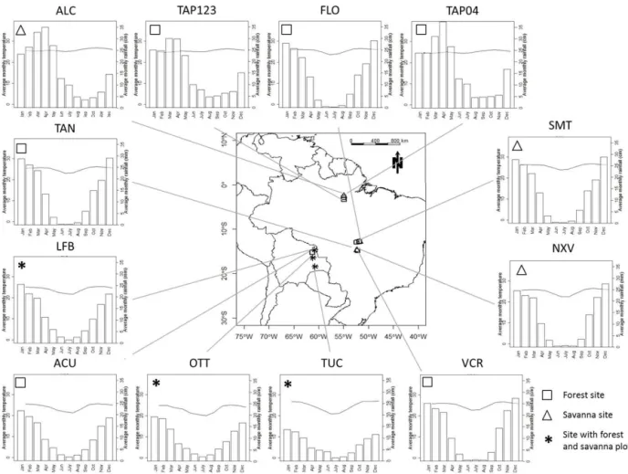
Figure 1. Map showing sampling sites and their temperature (◦C) and precipitation climatologies.
3. How do associated canopy structural characteristics such as leaf area, average and upper canopy tree heights and stand-level biomass vary with precipitation for for-est vs. savanna vegetation formation types?
4. And once variations in soil physical and chemical prop-erties have been taken into account – noting the likely importance of interactions with precipitation regimes – can we then account for variations in tropical forest and savanna structure using simple statistical models such as those applied in the forestry production literature? Or do variations in canopy structure in relation to climate remain so enigmatic that an invocation of “alternative stable states” becomes necessary?
2 Materials and methods 2.1 Study area
Data presented here come from 20 plots sampled in the southern and eastern areas of the Amazon Basin, and lo-cated in regions where both forest and savanna vegetation formation types were known to occur (Figs. 1 and 2). Most of
these plots were specifically sampled as part of the Tropical Biomes in Transition (TROBIT) project (Torello-Raventos et al., 2013), though with both plant and soil data for two forest plots (viz. TAP-123 and TAP-04) coming from previ-ous measurements made through the Amazon Rainforest In-ventory Network (RAINFOR) (Fyllas et al., 2009; Quesada et al., 2010, 2011). Additional photosynthesis and foliar N and P data for the forest plot TAP-04 come from Domingues et al. (2005). A list of all plots sampled along with selected climate and soil properties can be found in Supplement Ta-ble S1.
(a)
(b)
(c)
(d)
(e)
(f)
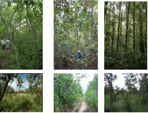
Figure 2. Examples of forest (top row) and savanna (bottom row) vegetation formation types found along the precipitation gradient. (a) TUC-01 forest, (b) TUC-03 savanna (both towards the drier end of the transect); (c) FLO-TUC-01 forest, (d) SMT-02 savanna (both in the middle of the Transect); (e) TAP-123 forest (f) ALC-02 savanna (both at the moister end of the transect). Specific details of site locations, climatology and soils are given in Fig. 1 and Table S1 of the Supplement.
2.2 Stand structure and species identification
Full details of canopy cover, tree height (H) and stand biomass estimates are provided in Torello-Raventos et al. (2013) and Veenendaal et al. (2015), and are thus only summarised briefly here. In short, we inventoried all trees and shrubs with a diameter (D) – at breast height (1.3 m) – of greater than 0.1 m with transect measurements being used for the estimation of size and abundance of smaller saplings, shrubs and seedlings (D >25 mm andH >1.5 m). Selected trees and shrubs in each plot were then used for determina-tion of site-specific allometric equadetermina-tions relating eitherHor estimated projected canopy areas (CA) toD. These equations were then used to estimate mean and 0.95 quantile heights (hereafter denoted ashHUi, andH∗, respectively) as well as stand-level crown area index,CW– defined as the sum of all woody individual canopy-projected area (including the sky-light transmitted component) divided by the ground area. Al-lometric equations employing some combination ofDand/or H and/or CA taken from a range of previously published sources or specifically developed as part of the TROBIT project were then used to estimate stand-level biomass (Vee-nendaal et al., 2015). Height and biomass estimates for the non-TROBIT forest plot TAP-123 comes from Feldpausch et al. (2011) with CW for TAP-123 and the nearby TAP-4 calculated from leaf area index measurements of these stands (Fyllas et al., 2014) using relationships given in Veenendaal
et al. (2015). Woody and herbaceous species were usually identified in the field by local botanists, but where necessary specimens were collected and verified against herbarium col-lections.
2.3 Soil physical and chemical properties
Soil sampling methods are described in detail in Quesada et al. (2010, 2011) and are thus only briefly summarised here. In brief, for each 1 hectare plot, five soil cores were col-lected and soil retained over the depths 0–0.05, 0.05–0.10, 0.10–0.20, 0.20–0.30, 0.30–0.50, 0.50–1.00, 1.00–1.50 and 1.50–2.00 m using an undisturbed soil sampler (Eijkelkamp Agrisearch Equipment BV, Giesbeek, the Netherlands). In addition, each plot usually had one soil pit dug to a depth of 2.0 m with samples collected from the pit walls at the same depths as above. Where possible, coring from the bot-tom of the soil pit for a further 2.0 m was also undertaken, giving a total maximum depth sampled of 4.0 m. All sam-pling was done following a standard protocol of RAIN-FOR network (http://www.geog.leeds.ac.uk/projects/rainfor/ pages/manualstodownload.html) in such a way to best ac-count for spatial variability within the plot.
2.3.1 Soil bulk density
Samples for bulk density determinations were taken from pit wall samples using specially designed container rings of known volume (Eijkelkamp Agrisearch Equipment BV, Giesbeek, the Netherlands) and subsequently oven dried at 105◦C until constant weight, cooled to room temperature in a sealed desiccant before final weight determinations were made. Three bulk density samples were collected at each sampling depth.
2.3.2 Soil texture and plant available soil water
Particle size analysis was performed using the pipette method (Gee and Bauder, 1986) with plant available soil water (θP) obtained through an estimation of soil water retention char-acteristics based on the particle size pedotransfer functions for tropical soils given by Hodnett and Tomasella (2002) for each sampled layer. Individual layer values (−0.01 to
−1.5 MPa) were then integrated to the maximum rooting depth for each profile or integrated to 4 m for the case of roots not having been observed to be constrained in any way. 2.3.3 Soil chemical properties
As described in detail by Quesada et al. (2010, 2011) sam-ples were analysed for pH in water at 1:2.5, with ex-changeable cations determined by the silver–thiourea method (Pleysier and Juo, 1980). Phosphorus pools were obtained from standard fractionation procedures as modified from Hedley et al. (1982). Soil carbon and nitrogen was deter-mined using an automated analyser (Pella, 1990; Nelson and Sommers, 1996). Samples from Bolivia were analysed in the School of Geography, University of Leeds, with those from Brazil at Instituto Nacional de Pesquisas da Amazonia in Manaus.
2.3.4 Plant available nutrients
As in Quesada and Lloyd (2015), the amount of nutrient available per unit ground area ([2]S,a) was estimated accord-ing to
[2]S,a=
z=d Z
z=0
ρb[2]ex,mdz, (1)
where[2]S,ais the soil nutrient content (expressed as g m−2 or mol m−2),ρbis the soil bulk density (typically in kg m−3),
[2]ex,mis the plant available soil nutrient on mass basis (typ-ically g g−1or mmol g−1),zis the soil depth (below the soil surface) anddis the depth of soil nutrient availability consid-ered, here – so as to be consistent with Quesada et al. (2012) – taken to be 0.3 m.
2.4 Leaf traits
Traits were assessed on an individual basis for at least 10 individuals with a diameter at breast height (1.3 m) greater than 0.1 m within each 1 ha plot. Trees were further selected on the basis that climbing the tree or cutting the branch from the ground could retrieve sun-exposed top-canopy branches. For each tree, a branch was harvested from the top canopy as described in Lloyd et al. (2010). A list of the species sam-pled is given in Table S2 along with details of the species’ as-sumed affinity (forest vs. savanna) and leaf habit – both these characteristics being mostly based on local botanical knowl-edge. In terms of leaf habit, trees were categorised as being deciduous (trees remain bare until leaf flush is induced by re-hydration), brevi-deciduous (short bare period in the dry season followed by leaf flush), semi-deciduous (trees losing old foliage as growth of new leaves starts) or evergreen (trees are never leafless but flush or shed leaves in regular periods or continuously throughout the year).
2.4.1 Leaf mass per unit area (Ma)
The ratio of fresh, one-sided area of a leaf to its dry weight was obtained by separating at least 10 healthy adult leaves from the bulk leaf sampled from each branch. Each leaf was then scanned using a flatbed scanner attached to a laptop as soon as possible after harvesting in the field. Where scan-ning on the day of collection was impossible due to logisti-cal reasons, leaves were stored in tightly sealed plastic bags under cool and dark conditions for a maximum of 2 days to avoid changes in the leaf area. The surface area of the leaf scans was subsequently analysed on an individual basis us-ing WinFOLIA™(Regent Instruments Inc., Ottawa, Canada). The scanned leaves were then oven dried to constant weight at 70◦C for about 24 h to prevent enzymatic decomposition, and their dry-mass determined after cooling in a desicca-tor. Where this was not possible due to logistical constraints, leaves were air dried in the field and oven dried as soon as possible.
2.4.2 Sample preparation
2.4.3 Carbon and nitrogen determinations
Foliar nitrogen[N]mand carbon[C]m in the bulk leaf sam-ples were determined on 15–30 mg of the ground plant mate-rial using elemental analysis (EURO EA CHNSO Analyser, HEKAtech GbhB, Wegberg, Germany in UoL and a CARLO ERBA EA 1110 CHN, Thermo Fisher Scientific, GmbH, Germany at CENA).
2.4.4 Cation and phosphorus determinations
At UoL, foliar cations (calcium, potassium and magnesium) and phosphorus in the ground samples were determined by inductively coupled plasma optical emissions spectrome-try (ICP-OES) (PerkinElmer Optima 5300DV, PerkinElmer, Shelton, CT, USA) following acid digestion (Lloyd et al., 2010). In the INPA laboratory, samples were digested us-ing a nitric–perchloric acid mixture, with concentrations of Ca, Mg and K determined using an Atomic Absorption Spectrophotometer (AAS) (Model 1100b, Perking Elmer, Norwalk, CT, USA) as described by Anderson and In-gram (1993) with phosphorus determined by Colorimetry (Olsen and Sommers, 1982) using a UV–visible spectropho-tometer (model 1240, Shimadzu, Kyoto, Japan). Sample di-lutions for AAS determinations were made with a 0.55 % lanthanum suppressant solution for Ca and Mg, with a 0.2 % CsCl solution for K. Details of solutions and standard series preparation can be obtained from Van Reeuwijk (2002). 2.4.5 Leaf construction costs
The cost of leaf construction (expressed as g glucose g−1 DW) was estimated as in Poorter and de Jong (1999), viz. K=(−1.041+5.077Cm)(1−φm)+5.325Norg, (2) whereKis the construction cost, Cmis the leaf carbon con-centration,φmis the leaf mineral content and Norgis the leaf organic N concentration (all in g g−1DW). For the purposes of calculation we assumed that all N present in the leaves was in the organic form (i.e. free nitrate levels were minimal as seems to be the case at least for Amazon forest species; Bloomfield, 2012), with leaf mineral content being approxi-mated as the sum of the measured major cations (Sect. 2.4.4). 2.4.6 Estimation of canopy nutrient concentrations The total amount of each nutrient contained in the foliage2C was estimated as (Quesada and Lloyd, 2015)
2C=Lh2mihMai, (3)
whereLis the stand leaf area index (D >0.1 m) taken from Veenendaal et al. (2015) –h2mi andhMaiare the species-abundance-weighted mass-based leaf nutrient estimates and leaf mass per unit area, respectively (see Sect. 2.6.2). Equa-tion (3) is by necessity an approximaEqua-tion – ignoring within
canopy gradients for example – also assuming a species’ abundance is also a good indication of its relative leaf area. But especially for comparison of canopy and soil available nutrient stocks, it does have advantages as compared to more simplistic approaches, such as in Cleveland et al. (2011), where variations in leaf area orMa are not even taken into account. Moreover, taken in conjunction with the “soil equiv-alent” (Eq. 1; Sect. 2.3.3), Eq. (3) allows both plant and soil nutrient stocks to be expressed on a per unit ground area basis (e.g. mol m−2), therefore providing a ready means for quan-titative comparisons.
2.5 Climatological data
Precipitation climatologies for all sites were obtained from the interpolated WorldClim data set (Hijmans et al., 2005). 2.6 Statistical analyses
2.6.1 Variance partitioning
As in Fyllas et al. (2009), the relative proportions of the total variance within the data set were apportioned to genetic, en-vironmental and “residual” components for each trait (2). Taking into account that the majority of species sampled could be assigned as being affiliated with either the forest (F) or savanna (S) biomes, the model fitted here was
2=A/S+p+ε, (4)
whereA represents the affiliation of species S (either for-est or savanna) located within plotp, andεis the residual variance: the nesting ofSwithinAallows for a splitting of the total between species variance into an intra- and inter-biome component. As noted by Fyllas et al. (2009), the resid-ual variance component includes any intra-species variability as well as any measurement error. These calculations were done using the “lme4” package (Bates et al., 2014) available within the “R” statistical platform (R-Development-Core-Team, 2014), treating all terms as random effects.
2.6.2 Variations in plot-level means in relation to vegetation type and precipitation
of h2iand associated weights so obtained were then inves-tigated in relation to variations in mean annual precipitation according to
h2i =µ+αS+s1(PA)+Ss2(PA), (5)
whereµrepresents the data set mean for trees located within the forest (F) vegetation type (i.e.V=F),Sis an indicator variable taking a value of 1 for all trees located within sa-vanna formations (for which by definition V6=F)and zero otherwise,s1is a non-parametric smoother, fitted to the data set as a whole, PA is the mean annual precipitation as es-timated for the plot in question and s2 is a non-parametric smoother defining the difference between forest and savanna vegetation formation types. Equation (5) thus allows for ferences in overall average trait values as well as for dif-fering interactions with precipitation for forest vs. savanna vegetation formation types: with these two aspects of varia-tion tested through a simplettest on the (fixed)αterm with s2(PA)=0 (i.e. an imposition of the same precipitation re-sponse on bothV), and a simpleF test evaluating the effect of inclusion of thes2(PA)term in Eq. (5; Zuur et al., 2009). For the fitting of Eq. (5), we used the “gam” function within the “mgcv” package (Wood, 2006, 2011) as available on the ”R” statistical platform (R-Development-Core-Team, 2014). Equation (5) was also used (without weights) in analyses of variations in bulked stand-level soil and canopy properties.
2.6.3 Soil–climate–vegetation associations
A variety of regression/correlation techniques were applied depending on the nature of the data and questions posed. These included ordinary least squares (OLS) regression, Kendall’s distribution-free test for independence (Hollan-der and Wolfe, 1999) and non-parametric (robust) regres-sion (McKean et al., 2009). All were undertaken using the “R” statistical platform (R-Development-Core-Team, 2014) using the “stats” or “Rfit” package (Kloke and McKean, 2013). For multivariate OLS regressions, variance inflation factors (VIF) were also calculated and are presented in the relevant tables along with the associated “tolerance” (i.e. 1/VIF). OLS regression coefficients are presented in both original and standardised form. The latter are presented as standardised values, this giving the relative change in the dependent variable per unit SD of each independent vari-able. Though potentially open to misinterpretation (Grace and Bollen, 2005), this provides a simple measure of the rel-ative importance of the various factors accounting for the variation in stand structure or physiological variables in-vestigated, the standardising factor being the variability (af-ter transformation where appropriate) of the various candi-date independent variables along the precipitation transect as measured by our data set.
3 Results
3.1 Soil properties
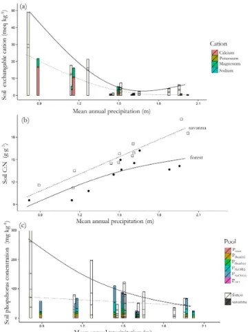
Across the precipitation (PA) gradient, forest soils had an exchangeable base cation content (usually referred to as the “sum of bases”:[Ca]ex+ [K]ex+ [Mg]ex+ [Na]ex=6B) greater than the savanna soils (Fig. 3a) as reflected by an esti-matedα= −9.1±3.1 mmol kg−1for the model fit of Eq. (5) (p=0.010). That analysis also showed a difference between the twoVin their overall precipitation dependencies with the “s2” term in Eq. (5) being significant atp=0.005; i.e. the forest (F) and savanna (S) soils differed both in their overall average6Band in the way that6Bvaried with precipitation. For bothV,6B were clearly higher at lowPA. Across the precipitation gradient individual cation concentrations were typically [Ca]ex>[Mg]ex [K]ex for any individual plot, with[Ca]exand[Mg]exincreasing more markedly with de-cliningPAthan was the case for[K]ex(see Table S1 for ac-tual values).
Soil C/N ratios (CNs)also varied with both V and PA (Fig. 3b) withSsoil being on average 2.3±0.6 g g−1higher than forFsoils (p≤0.001). In both cases, CNsdeclined with decreasing PA with (after accounting for intercept differ-ences) no apparent difference between the two fitted curves (p=0.155).
Extractable soil phosphorus concentrations, [P]extr, also showed a dependence upon bothV andPA (Fig. 3c) with markedly lower values in savanna sites as reflected in the fitted value ofαin Eq. (5) being−143±44 mg kg−1(p=
0.005). There was also a clear difference between FandS in the way[P]extrvaried with precipitation (p=0.023) with the lack of any clear savannaPAdependency (p=0.58) in marked contrast to the increasing forest[P]extrasPAdeclined (for whichp <0.001). In all soils, the bulk of the[P]extrpool was made up of the less accessible NaOH extractable organic and inorganic fractions (PNaOH(o)and PNaOH(i), respectively). Small amounts of mineral P were also present in some of the lowerPA soils as indicated through the presence of an HCl extractable component.
Figure 3. Variations in key soil chemical properties (0.0–0.3 m depth) in relation to precipitation and vegetation formation type (a) soil exchangeable cations; (b) soil C/N ratio; (c) soil phos-phorus pools. For (a) and (b) forest plots are shaded more lightly than savanna with the fitted curves (solid for forest plots, dashed for savanna) representing generalised additive model fits represent-ing for (a) total exchangeable cations (sum of bases) and for (c) total extractable phosphorus. In (c) the phosphorus pools are as per the Hedley fractionation procedure (see Sect. 2.3.3): [P]resin – resin extractable P; [P]Bicarb(i) – bicarbonate extractable in-organic phosphorus; [P]Bicarb(o) bicarbonate extractable organic phosphorus;[P]NaOH(i)– NaOH extractable inorganic phosphorus; [P]NaOH(o) bicarbonate extractable organic phosphorus;[P]HCl – HCl extractable phosphorus.
3.2 Canopy characteristics
All three canopy structural properties showed differences both in absolute values and precipitation dependencies for forest vs. savanna plots (Figs. 2 and 4). Specifically, there was a clear decline in forest canopy area index (CW) with declining precipitation (p <0.001), but with the best-fit line for savanna plots (which were on average of a lower CW than their forest counterparts) only significant atp=0.183 (Fig. 4a).
Also observed was a tendency for the increase in 0.95 quantile canopy height with rainfall to approach its maxi-mum at highPA(overall response significant atp <0.001)
but with no systematic dependency ofH∗onPAforS(p= 0.106): the trees in savanna plots being on average 10.5 m shorter than their forest counterparts (Fig. 4b).
Above-ground biomass (BU) estimates showed similar patterns forCWandH∗(Fig. 4c), although in this case (in-terestingly) with the slight increase in savannaBUasPA de-clines, statistically significant atp <0.001.
Overall, we find a marked decline in stature and canopy area with precipitation for forest sites but not for savannas. Thus, savanna and forest are much more similar in their above-ground structural characteristics at lowerPA.
3.3 Leaf traits
3.3.1 Variance partitioning (mass-based traits)
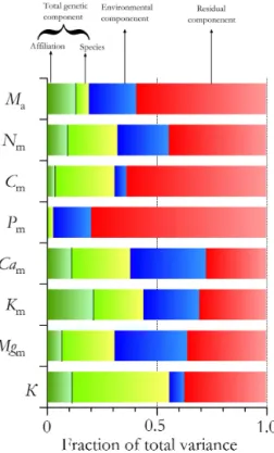
Through fitting the multilevel model of Eq. (4), a partition-ing of the variance to genetic- and plot-level components was achieved with results presented for leaf mass per unit area (Ma), mass-based nutrient concentrations and estimated leaf construction costs (Eq. 2) shown in Fig. 5. Here, because each species could be assigned as primarily affiliated with ei-ther forest or savanna, it was furei-ther possible to partition the genetic component into that systematically associated with where a species typically grows (its “affiliation”) as opposed to genetic variation within the forest and savanna grouping themselves. This analysis shows not only that relative contri-butions of the genetic-components vs. the plot-components vary from trait to trait, but also that the relative magnitude of the residual component (representing within-species vari-ability and experimental error) is trait dependent.
The genetic component that is systematically associated with a species’ affiliation was typically a small proportion of the overall variability, the one exception being for potassium (Km) where the relative contributions were approximately equal. With the exception of phosphorus (Pm), the variance explained by the combined genetic components was of equal or greater magnitude than the plot-dependent (environmen-tal) component with the latter being only a minor contributor to the overall variations in Cm and the associated leaf con-struction costs (K).
Figure 4. Variations in canopy structural properties in relation to precipitation and vegetation formation type (a) canopy area index, (b) upper 0.95 quantile height and (c) above-ground biomass. (•) Forest plots; () savanna plots. Fitted curves (solid for forest plots, dashed for savanna) represent generalised additive model fits.
Figure 5. Partitioning of the total variance for mass-based foliar properties into genetic (green), environmental (blue) and residual (red) components with the genetic component further divided into the variations between versus within vegetation formation affilia-tion (each species having being identified as principally associated with either forest or savanna).Madenotes mass per unit area and K represents leaf construction costs. Other symbols represent the elemental composition of the leaves on a dry-mass (subscript “m”) basis.
Cm, Mgm, and K all having savanna species mean values all within 20 % of the forest species’ mean) but with Cam and Kmshowing much larger differences (savanna affiliated species showing reductions of 34 and 39 %, respectively, as compared to forest species: Table S3).
3.3.2 Mass-based trait variation in relation to vegetation type and precipitation
Across the precipitation gradient, leaves of trees within sa-vanna formations (S) had consistently higher leaf mass per unit area than those where the dominant species mix con-sisted of forest species (F; Fig. 6a). From the generalised additive model fit (Eq. 5), this overallhMaidifference (α= 32±9 g m−2) was significant atp=0.001. Overall, thePA dependencies observed were highly significant atp <0.001 for bothV, but the differing fitted trends were not so sig-nificant (p=0.183); i.e. little credence should be placed on the greater difference between the two vegetation formation types at the highestPA.
For stand-level leaf nitrogen there was also an obvious dif-ference in overall concentrations between the twoV(F−S= 6.0±1.5 mg g−1;p=0.001; Fig. 6b) with the fitted precip-itation dependencies showing an increase with decliningPA significant atp <0.001 andp=0.065 forFandS, respec-tively. As forhMaithere was, however, no difference in the fittedPAdependencies forhNmionce differences in absolute values were taken into account (p=0.588). Thus, after ac-counting for differences in intercept both forest and savanna can be considered as showing similar increases inhNmiwith decliningPA.
Figure 6. Variations in community-abundance-weighted mean fo-liar properties in relation to precipitation and vegetation formation type (a) leaf mass per unit area, (b) leaf nitrogen (dry-mass basis), (c) leaf phosphorus (dry-mass basis) and (d) carbon (dry-mass ba-sis). (•) Forest plots; () savanna plots. Fitted curves (solid for for-est plots, dashed for savanna) represent generalised additive model fits. Error bars represent the community-abundance-weighted SD.
A similar lack of any effect of vegetation formation type was also observed for leaf carbon concentrations (Fig. 6d) where althoughhCmiwere 11 mg g−1higher forSplots this effect was significant only atp=0.091. The fittedPA de-pendencies were, nevertheless, significant at p <0.001 in both cases, but also not different in pattern to each other (p=0.687).
Despite the hCami differences between F andS plots at lowerPA, the overall contrast (F−S) of 1.4 mg g−1was only significant at p=0.161, presumably a consequence of sig-nificant overlap between the two V at around PA=1.5 m and the high variance of the community-weighted means at higher overall hCami, especially for forest plots at low PA (Fig. 7a). The fittedPAdependencies were highly significant in both cases (p <0.001), but with overall patterns not dif-ferent (p=0.687).
ForhKmi,FandSvalues were significantly different over-all (p=0.015) with savanna plots being estimated as, on
Figure 7. Variations in community-abundance-weighted mean fo-liar properties in relation to precipitation and vegetation formation type (a) leaf calcium mass basis), (b) leaf potassium (dry-mass basis), (c) leaf magnesium (dry-(dry-mass basis) and (d) leaf con-struction costs. (•) Forest plots; () savanna plots. Fitted curves (solid for forest plots, dashed for savanna) represent generalised ad-ditive model fits. Error bars represent the community-abundance-weighted SD.
average, 1.8±0.7 mg g−1 less than forest (Fig. 7b). Over-all fittedPA dependency patterns – which were significant atp <0.001 andp=0.025 forFandS, respectively – were also appreciably different from each other (p=0.010). Thus forhKmiwe can conclude that forFthe rate of increase with declining precipitation was more or less constant across the transect. This is opposed to S where the increase in hKmi with decliningPA was more moderate, also occurring only towards the drier end of the transect.
Overall, the 0.67 mg g−1 lower hMg
mi observed for the savanna plots (Fig. 7c) did not make them appreciably dif-ferent to their forest counterparts (p=0.155) with no dif-ference between the twoVin the nature of theirPA depen-dencies (p=0.192), which were themselves both significant (p=0.001 andp=0.047 forFandS, respectively). As for
Leaf construction costs showed a slight overall depen-dence on V with hKi for S being on average 0.077±
0.037 mg glucose g−1DW higher than
F (p=0.053). Al-though the individually fitted curves are different in form for F vs. S (Fig. 7d) this difference in shape is not of conse-quence (p >0.999).
Although a lack of knowledge for many of the species studied prevents rigorous inferences of trends in leaf habit, from those species for which this information was avail-able (Tavail-able S2), it can be confidently stated that at the dri-est Tucavaca sites in Bolivia that all species were decidu-ous (both forest and savanna) with semi-decidudecidu-ous and brevi-deciduous and then evergreen species becoming more com-mon as precipitation increased. At all sites other than Tu-cavaca, evergreen species were more common in the forests and purely deciduous species more common in the savanna. 3.3.3 Vegetation–soil nutrient associations
Estimates on canopy nutrient contents (Eq. 2) as a function of soil exchangeable nutrient contents (Eq. 1) showed no clear relationship for calcium (CaC; Fig. 8a), magnesium (MgC; Fig. 8b) and phosphorus (PC; Fig. 8d), but with some asso-ciation being more clear for potassium (KC; Fig. 8c). Us-ing a robust regression procedure (relatively immune to out-liers), significance levels as estimated through a dispersion test werep=0.062, 0.266, 0.026 and 0.402 for CaC, MgC, KC, and PC, respectively.
As the graphs of Fig. 8 express both plant and soil nu-trients on the same per unit ground area basis, they provide a ready means to evaluate the relative amounts of any nutrient in the foliage vs. the soil. Here we then see that, as approach-ing the asymptote, CaC'0.1[Ca]sa, MgC'0.1[Mg]sa and PC'0.08[P]sa, but for KC: [K]sa there is no real flattening out, with canopy potassium contents quite similar to those of calcium and magnesium despite much lower soil concentra-tions; i.e. relative to the amount of soil nutrient present, there is much less K in the canopy foliage than is the case for Ca and Mg. This is in addition to a much clearer relationship be-tween the nutrient stocks in the canopy vs. soil pools for K than for the other cations examined. For phosphorus the gen-erally overall lower canopy foliar contents of savanna plots are not associated with a lower[P]sa.
3.4 Photosynthesis and related traits
3.4.1 Variance partitioning (area-based traits)
In contrast to the mass-based traits, in no case was the pro-portion of the total data set variance in light and CO2 sat-urated assimilation rates (Amax), area-based nitrogen and phosphorus concentrations (Naand Pa, respectively), photo-synthetic N and P use efficiencies (ANandAP, respectively) and foliarδ13C attributable to species affiliation per se. But still – with the exception of Pa, and to a lesser extentδ13C –
Figure 8. Relationships between soil and community-abundance-weighed foliar nutrient concentrations with both expressed on a ground area basis. (a) Calcium, (b) magnesium, (c) potassium and (d) phosphorus. (•) Forest plots; () savanna plots. The curves shown are log-linear, viz.y=a+blog(x), fitted using a robust non-parametric procedure.
a notable portion of the explained variance was attributable to species identity. Plot identity as estimated through the en-vironmental components was also an appreciable source of variation in all cases, especially forδ13C and – in relative terms – also for Pa.
3.4.2 Area-based trait variation in relation to vegetation type and precipitation
Stand-level species-abundance-weighted maximum CO2 as-similation rates (Fig. 10a) did not vary overall between the twoV(p=0.851), nor – despite their fitted slopes being of a different sign – did their precipitation dependencies differ (p=0.302). Amongst this general “noise” of note, however, are two noticeably highhAmaxiplots: the relatively low pre-cipitation forest OTT-01 and the mid-prepre-cipitation savanna LFB-03.
dependen-Figure 9. Partitioning of the total variance for photosynthesis-associated foliar properties into genetic (green), environmental (blue) and residual (red) components with the genetic component further divided into the variations between versus within vegetation formation affiliation (each species having being identified as princi-pally associated with either forest or savanna).Amaxdenotes light and CO2saturated (maximum) CO2assimilation rate; Naand Pa represent the nitrogen and phosphorus composition of the leaves on an area (subscript “a”) basis;AN andAPrepresent the photosyn-thetic nitrogen and phosphorus-use efficiencies (viz.Amax/Naand Amax/Pa) withδ13C a measure of the leaf13C/12C composition.
cies (p=0.006). Specifically, there was virtually no sys-tematic variation ofhNaiwith precipitation for the savanna plots, but with an increase in forest plothNaiasPAdecreased (p <0.001).
For hPai there was a small effect of V on mean values (Fig. 10c) with savanna plots typically being 0.022 g m−2 higher than their forest counterparts. As forhAmaxiandhNai, opposing patterns of variations withPAwere observed, here with a decline inhPaicoinciding with an increase in precipi-tation forF, but with less pattern observed forS.
Finally, we note the clear contrasting patterns in hδ13Ci
observed for F vs. S with a more or less constant decline with increasing precipitation observed for the forest plots, but with this pattern only being replicated for savanna plots at lowerPA(Fig. 10d). Here the fitted curves were both sig-nificant atp <0.001 and statistically different to each other (p=0.011).
Figure 10. Variations in community-abundance-weighted mean fo-liar properties in relation to precipitation and vegetation formation type (a) light and CO2saturated (maximum) CO2assimilation rate, (b) leaf nitrogen (area basis), (c) leaf phosphorus (area basis) and (d) leaf13C/12C composition. (•) Forest plots; () savanna plots. Fitted curves (solid for forest plots, dashed for savanna) represent generalised additive model fits. Error bars represent community-abundance-weighted SD.
3.4.3 Identifying key drivers of variation inhAmaxiand hδ13Ci
With Fig. 10 suggesting broad-scale interacting patterns of variations in hAmaxi withV and PA quite similar in form tohNaiandhPai, Kendall’s non-parametric regression coef-ficients (τ) were calculated for these and other stand-level properties of interest (Table 1). This shows that, contrary to expectation, the only significant univariate correlation with
hAmaxiatp <0.05 was a negative one with soil potassium. Consequently [K]sa also exhibited strong positive correla-tions with a range of stand-level structural properties such as crown area index and canopy height (both mean and 0.95 quantile) as well ashδ13Ci.
Table 1. Kendall’s bivariate correlation coefficients for stand-level photosynthetic capacityhAmaxi, photosynthetic nitrogen use efficiency hANi, photosynthetic phosphorus-use efficiencyhAPiand their association with a range of canopy, soil and climatic factors, viz. community-weighted means of area-based leaf nitrogenhNaiand phosphorushPaiconcentrations; leaf carbon stable isotopic compositionhδ13Ci; total woody canopy area indexCW; upper 0.95 quantile upper-canopy heighthHUi; community-weighted mean upper-canopy heightH∗; area-based measures of soil nutrient availability for calcium, potassium and magnesium, viz.[Ca]sa,[K]saand[Mg]sa; soil carbon/nitrogen ratio (CN), and mean annual precipitation (PA). Values significant atp <0.05 are shown in bold.
hAmaxi 0.65 hANi 0.43 0.54 hAPi 0.17 −0.18 −0.12 hNai −0.12 −0.26 −0.7 0.22 hPai −0.09 −0.27 −0.29 0.25 0.31 hδ13Ci −0.07 −0.02 0.11 0.08 −0.2 0.01 CW
0.01 0.08 0.20 0.16 −0.25 0.02 0.74 hHUi −0.01 0.06 0.22 0.16 −0.26 0.02 0.73 0.86 H∗
−0.13 −0.3 −0.15 0.20 0.05 0.53 0.13 0.13 0.18 [Ca]sa −0.37 −0.42 −0.15 0.20 0.01 0.32 0.42 0.37 0.42 0.53 [K]sa −0.15 −0.29 −0.09 0.19 −0.03 0.38 0.12 0.10 0.16 0.85 0.54 [Mg]sa −0.05 −0.12 0.03 0.12 −0.1 0.31 0.14 0.08 0.17 0.50 0.52 0.53 [P]sa
0.15 0.22 −0.07 −0.07 0.28 −0.2 −0.05 −0.16 −0.15 −0.53 −0.41 −0.56 −0.38 CNs 0.2 0.35 0.05 −0.13 0.16 −0.25 0.06 0.03 −0.01 −0.46 −0.37 −0.59 −0.43 −0.85 PA
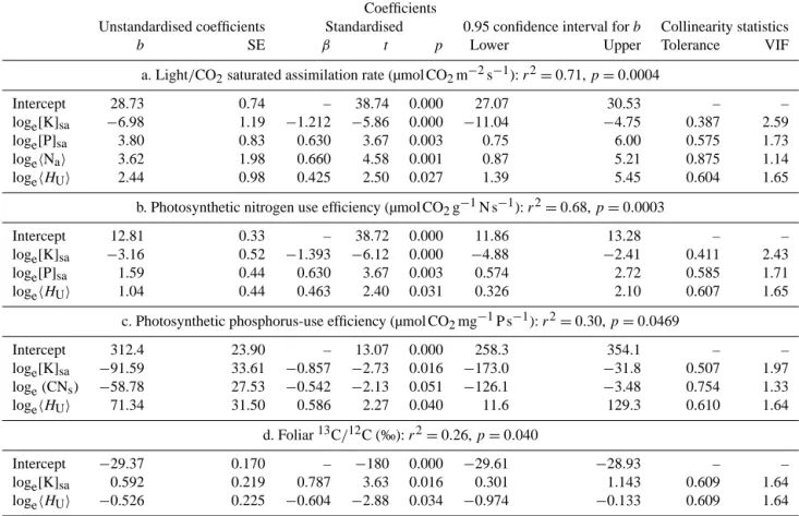
log relationship ofhAmaxiwith[K]sa,[P]sa,hNaiandhHUi was found, details of which are given in Table 2a. Here, along with unstandardised coefficients, standardised values are also given together with the appropriate collinearity statistics, the latter giving VIF<10 (tolerance>0.1), which suggests that cross-correlations between predictor variables were not an issue in the model fit. From the standardised coefficients we can conclude that the dominant effect is, indeed, the nega-tive[K]saassociation and the other three positive factors, viz.
[P]sa,hNaiandhHUiall contributing to a lesser degree. The reasons for the complex multivariate association can be seen in Fig. 11, wherehAmaxiis individually plotted as a function of each of [K]sa,[P]sa,hNai andhHUi. Here, for example, although the forest plot OTT-01 is a clear outlier when con-sidered just in terms of [K]sa, this apparently anomalously highhAmaxi can, however, be explained in terms of a very highhNai. The lower precipitation forest plot TUC-01 also has a highhNai, but in this case[K]sais very high andhHUi relatively low: these factors then combine (at least according to the model) to give a relatively lowhAmaxi. For the savanna plot LFB-03, the main contributing factor to its highhAmaxi is suggested by the model to arise through a very low[K]sa
combined with a reasonably high[P]sa.
Given the relatively strong association between soil ex-changeable K and the other base cations (Table 1), it was of interest to see if these could substitute for potassium as a predictor of hAmaxi with other potentially important soil properties, such as pH and soil and clay content, also be-ing tested. This analysis confirmed potassium as the definbe-ing soil predictor, with the best alternative predictor, as detected through a substitution of the[K]saterm in the model of Ta-ble 2a, being the[Mg]sa term with anr2of only of 0.15 (cf. 0.71 for[K]sa). This “best alternative model” had an Akaike’s
information criterion (AIC) of 117.6 as compared to 98.4 for the equation in Table 2a.
Soil potassium status was also negatively related to species-abundance-weighted photosynthetic nitrogen use ef-ficiency; hANi = hAmax/Nai; indeed, following a similar procedure as forhAmaxi, significant associations atp <0.05 were again found for [K]sa, [P]sa and hHUi with soil ex-changeable potassium again the dominant (negatively associ-ated) predictor variable (Table 2b). As forhAmaxi, alternative soil predictors gave a markedly inferior fit, the “best alterna-tive model” again being with[Mg]sa but with anr2only of 0.15 (cf. 0.68 for[K]sa). This model had an AIC of 87.1 as compared to 68.7 for the equation in Table 2b. In both the above cases, substituting either the soil[K]sa variable with its canopy equivalenthKaiand/or the soil[P]savariable with its canopy equivalenthPaialso gave rise to a markedly infe-rior fit (data not shown).
This was similar in the case of a fit of species-abundance-weighted photosynthetic phosphorus-use efficiency;hAPi =
hAmax/Pai, where soil C : N was a significantly better pre-dictor thanhNai with[K]sa andhHUi again included in the best-fit model (Table 2c). Here again, other soil properties could not be substituted for[K]sa with the best alternative predictor being[Ca]sa giving an AIC of 226.7 as compared to 222.8 for the equation in Table 2c.
Soil exchangeable potassium also showed a relatively high Kendall’s τ when considered as a univariate predictor of
hδ13Ci (Table 1); indeed, a model consisting of [K]sa and
Table 2. Multivariate regression statistics relating estimates of community-weighted canopy-level average maximum CO2assimilation rates, nitrogen use efficiency, phosphorus-use efficiency and foliar13C/12C to canopy and soil variables. Abbreviations:[K]sa – soil potassium (mmol m−2),[P]sa(µmol m−2),hNai– species-abundance-weighted area-based leaf nitrogen (g m−2),hHUi– average canopy height (trees> 0.1 m diameter at beast height, in m), CNs – soil CN ratio (g g−1) and VIF – variance inflation factor. In all cases predictor variates have been centred with the unstandardised intercept giving then the predicted value when all predictor variables are at their mean values. In the standardised case, all variables have been centred and scaled by their SD.
Coefficients
Unstandardised coefficients Standardised 0.95 confidence interval forb Collinearity statistics
b SE β t p Lower Upper Tolerance VIF
a. Light/CO2saturated assimilation rate (µmol CO2m−2s−1):r2=0.71,p=0.0004
Intercept 28.73 0.74 – 38.74 0.000 27.07 30.53 – –
loge[K]sa −6.98 1.19 −1.212 −5.86 0.000 −11.04 −4.75 0.387 2.59 loge[P]sa 3.80 0.83 0.630 3.67 0.003 0.75 6.00 0.575 1.73
logehNai 3.62 1.98 0.660 4.58 0.001 0.87 5.21 0.875 1.14
logehHUi 2.44 0.98 0.425 2.50 0.027 1.39 5.45 0.604 1.65
b. Photosynthetic nitrogen use efficiency (µmol CO2g−1N s−1):r2=0.68,p=0.0003
Intercept 12.81 0.33 – 38.72 0.000 11.86 13.28 – –
loge[K]sa −3.16 0.52 −1.393 −6.12 0.000 −4.88 −2.41 0.411 2.43 loge[P]sa 1.59 0.44 0.630 3.67 0.003 0.574 2.72 0.585 1.71 logehHUi 1.04 0.44 0.463 2.40 0.031 0.326 2.10 0.607 1.65
c. Photosynthetic phosphorus-use efficiency (µmol CO2mg−1P s−1):r2=0.30,p=0.0469
Intercept 312.4 23.90 – 13.07 0.000 258.3 354.1 – –
loge[K]sa −91.59 33.61 −0.857 −2.73 0.016 −173.0 −31.8 0.507 1.97 loge(CNs) −58.78 27.53 −0.542 −2.13 0.051 −126.1 −3.48 0.754 1.33 logehHUi 71.34 31.50 0.586 2.27 0.040 11.6 129.3 0.610 1.64
d. Foliar13C/12C (‰):r2=0.26,p=0.040
Intercept −29.37 0.170 – −180 0.000 −29.61 −28.93 – –
loge[K]sa 0.592 0.219 0.787 3.63 0.016 0.301 1.143 0.609 1.64 logehHUi −0.526 0.225 −0.604 −2.88 0.034 −0.974 −0.133 0.609 1.64
hHUi(r2=0.383) giving an AIC of 40.7 as compared to 44.1 for the equation in Table 2c.
Especially asPA, on its own showed a reasonably strong correlation with[K]sa (Table 1); mean annual precipitation was also tested as a predictor variable forhAmaxi,hANi,hAPi andhδ13Ci. But in no case, either on its own or in conjunction with the other predictor variables in Table 2, did it give rise to anr2even closely approximating[K]sa(data not shown). 3.5 Predicting canopy structural properties
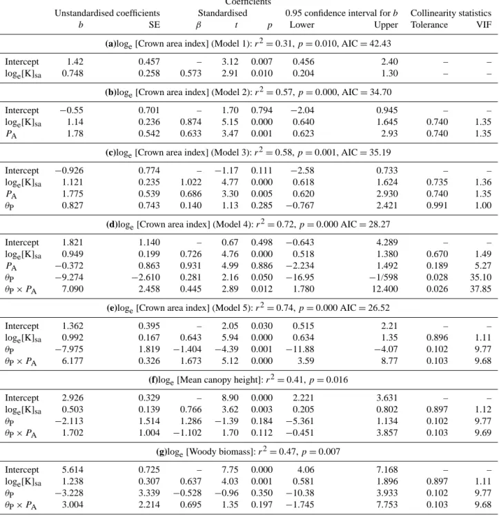
In addition to an important role as a modulator of leaf-level photosynthetic properties, Table 1 also suggests a strong as-sociation between [K]sa and CW and both canopy height measures. With CW relating directly to both leaf area in-dex and fractional canopy cover (Veenendaal et al., 2015) and both providing commonly used measures of woody plant plenteousness in tropical ecosystems (Lloyd et al., 2008; Hi-rota et al., 2011; Staver et al., 2011; Murphy and Bowman, 2012; Torello-Raventos et al., 2013; Veenendaal et al., 2015), we therefore first applied a simple OLS log–log model
Table 3. Multivariate regression statistics relating canopy area index (CW), mean upper stratum canopy heighthHUi, and above-ground biomass (BU) to soil and climatic variables. From (a) to (d) occur increasingly complex models for the prediction ofCW; (e) represents an application of model (d) tohHUiand (f) is model (d) but applied toBU. Other abbreviations:[K]sa– soil potassium (mmol m−2),PAmean annual precipitation (m), VIF – variance inflation factor. In all cases predictor variates have been centred with the unstandardised intercept giving then the predicted value when all predictor variables are at their mean values. In the standardised case, all variables have been centred and scaled by their SD.
Coefficients
Unstandardised coefficients Standardised 0.95 confidence interval forb Collinearity statistics
b SE β t p Lower Upper Tolerance VIF
(a)loge[Crown area index] (Model 1):r2=0.31,p=0.010, AIC=42.43
Intercept 1.42 0.457 – 3.12 0.007 0.456 2.40 – –
loge[K]sa 0.748 0.258 0.573 2.91 0.010 0.204 1.30 – –
(b)loge[Crown area index] (Model 2):r2=0.57,p=0.000, AIC=34.70
Intercept −0.55 0.701 – 1.70 0.794 −2.04 0.945 – –
loge[K]sa 1.14 0.236 0.874 5.15 0.000 0.640 1.645 0.740 1.35
PA 1.78 0.542 0.633 3.47 0.001 0.623 2.93 0.740 1.35
(c)loge[Crown area index] (Model 3):r2=0.58,p=0.001, AIC=35.19
Intercept −0.926 0.774 – −1.17 0.111 −2.58 0.733 – –
loge[K]sa 1.121 0.235 1.022 4.77 0.000 0.618 1.624 0.735 1.36
PA 1.775 0.539 0.686 3.30 0.005 0.620 2.930 0.740 1.35
θP 0.827 0.743 0.140 1.13 0.285 −0.767 2.421 0.991 1.00
(d)loge[Crown area index] (Model 4):r2=0.72,p=0.000 AIC=28.27
Intercept 1.821 1.140 – 0.67 0.498 −0.643 4.289 – –
loge[K]sa 0.949 0.199 0.726 4.76 0.000 0.518 1.380 0.670 1.49
PA −0.372 0.863 0.931 4.99 0.886 −2.234 1.492 0.189 5.27
θP −9.274 −2.610 0.281 2.16 0.050 −16.95 −1/598 0.028 35.10 θP×PA 7.090 2.458 0.445 2.89 0.012 1.780 12.400 0.026 37.85
(e)loge[Crown area index] (Model 5):r2=0.74,p=0.000 AIC=26.52
Intercept 1.362 0.395 – 2.05 0.030 0.515 2.21 – –
loge[K]sa 0.992 0.167 0.643 5.94 0.000 0.634 1.35 0.896 1.11 θP −7.975 1.819 −1.404 −4.39 0.001 −11.88 −4.07 0.102 9.77
θP×PA 6.177 0.326 1.673 5.12 0.000 3.59 8.77 0.103 9.68
(f)loge[Mean canopy height]:r2=0.41,p=0.016
Intercept 2.926 0.329 – 8.90 0.000 2.221 3.631 – –
loge[K]sa 0.503 0.139 0.766 3.62 0.003 0.205 0.802 0.897 1.12
θP −2.113 1.514 1.286 −1.39 0.184 −5.361 1.134 0.102 9.77
θP×PA 1.702 1.004 −1.102 1.70 0.112 −0.451 3.857 0.103 9.69
(g)loge[Woody biomass]:r2=0.47,p=0.007
Intercept 5.614 0.725 – 7.75 0.000 4.06 7.168 – –
loge[K]sa 1.238 0.307 0.637 4.03 0.001 0.581 1.896 0.897 1.11 θP −3.228 3.339 −0.528 −0.96 0.350 −10.38 3.933 0.102 9.77 θP×PA 3.004 2.214 0.695 1.35 0.197 −1.745 7.753 0.103 9.68
Overall, predictions ofCWaccording to Model 5 were of acceptable fidelity (Fig. 12a) with the wide range of savanna CWwell predicted, in particular by this simple mixture of soil chemical and hydrological properties. Some differentiation of the forest plots would also seem to have been achieved by
the model. Nevertheless, there was a tendency for the model to under-predict forestCWand vice versa for savanna plots.
Figure 11. Relationships of community-abundance-weighted mean maximum CO2assimilation rates to (a) soil exchangeable potas-sium, community-abundance-weighted foliar nitrogen concentra-tions (area basis), (c) soil available phosphorus and (d) mean canopy height. Selected plots (specifically mentioned in the text) are also shown. (•) Forest plots; () savanna plots.
the symbol size relates to[K]sa. From Fig. 12b it can be seen that in any one region of the plot that the smaller symbols (lower [K]sa) tend to be of a redder hue (lower CW), and consideration of similarly sized symbols shows a tendency for increased greenness (higherCW) as one moves along the main diagonal. Reddish symbols (of lowCW) are typically smaller (of lesser[K]sa) at higherPA, although the pattern of variation withθPis less systematic.
As an illustration, model predictions of canopy area index (CˆW) variations as a function of[K]sa are shown in Fig. 12c for PA=1.0 m a−1 and PA=1.5 m a−1 (θP=0.5 m). This shows the model to be especially responsive to[K]sa below about 0.2 mol m−2with a greater sensitivity ofCˆ
Wto[K]saat higherPA. Thus, in relative terms,CˆWis modelled to become most sensitive toPAat low[K]sa.
Figure 12d–f show how the PA×θP interaction affects
ˆ
CW at three different [K]sa. Here (where white areas are for CˆW<0 and for which we therefore assume in practice CW=0) we see first for Fig. 12d that at a very low[K]saof 0.1 mol m−2the model suggests that any sort of woody leaf area is simply not possible forPA<1.5 m a−1, and even then
only whenθP is relatively high. AsPA increases, theθP for whichCˆ
W>0 increases, with aCˆW of around 2 m2m−2at the highestPA–θPcombination examined considered possi-ble.
At double potassium availability with [K]sa=
0.2 mol m−2, the response observed is very different (Fig. 12e). Here, by comparison with Fig. 12d, we can again see the generally higherCˆWanticipated for the higher PA–θPcombinations. But at aroundPA'1.3 m a−1, the area delineated by theCˆW=0 shifts from a concave to a convex form; i.e. the model then predicts that forPA/1.3 m a−1, rather than an increaseCW should decline with increasing θP.
At an even higher [K]sa of 0.4 mol m−2 the general concave–convex pattern is maintained (Fig. 12f) with higher
ˆ
CW at all PA–θP combinations. The domain for which
ˆ
CW>0 is also shifted compared to Fig. 12e with additional combinations of lowerPA/higherθP also deemed possible. At the lowest simulated PA of 0.8 m a−1, CˆW>0 is now modelled as possible for allθPless than about 0.5 m.
Application of Model 5 to other structural variables also gave rise to a reasonable fit. For example, as shown in Ta-ble 3f, a reasonaTa-ble fit ofr2=0.41 was found whenhHUi was substituted as the dependent variable. Above-ground biomass (BU) was also reasonably well predicted by the model (Table 5g:r2=0.47), in both cases with a role for potassium still evident atp=0.001.
When taken in conjunction withPA andθP,[K]safurther proved to be a much better predictor for each of the three structural variables examined than any other measured soil property. For example, the next-best alternative to[K]sa as a co-predictor forCW in Model 5 was[Mg]sa, which gave ar2=0.65 and an AIC =31.9 as compared to r2=0.74 and AIC=26.5 for[K]sa (Table 2e). For bothhHUiandBU it also emerged that[Mg]sa was the next-best substitute for
[K]sa, but in both cases with the differences between the two cations in their statistical efficacy much less marked with 1AIC= −0.4 forhHUiand−1.9 forBU.
3.6 Soil water simulations